Abstract
The explosive growth of power load data has led to a substantial presence of abnormal data, which significantly reduce the accuracy of power system operation planning, load forecasting, and energy usage analysis. To address this issue, a novel improved GAN–Transformer model is proposed, leveraging the adversarial structure of the generator and discriminator in Generative Adversarial Networks (GANs). To provide the model with a suitable feature dataset, One-hot encoding is introduced to label different categories of abnormal power load data, enabling staged mapping and training of the model with the labeled dataset. Experimental results demonstrate that the proposed model accurately identifies and classifies mutation anomalies, sustained extreme anomalies, spike anomalies, and transient extreme anomalies. Furthermore, it outperforms traditional methods such as LSTM-NDT, Transformer, OmniAnomaly and MAD-GAN in Overall Accuracy, Average Accuracy, and Kappa coefficient, thereby validating the effectiveness and superiority of the proposed anomaly detection and classification method.
1. Introduction
The rapid development and deployment of massive distributed renewable energy sources, electric vehicles, charging stations, distributed energy storage systems, and various types of smart terminals are occurring at a fast pace in power systems. These devices, located at the end of the perception layer, generate an enormous amount of monitoring data continuously, characterized by an exponential growth pattern [1]. Power load data describe the magnitude of energy consumption, variation trends, and distribution characteristics of load objects within a specific range. Meanwhile, power load data serve as a core asset that reflects the load level of the power system and supports the operational planning, intelligent management of the power system, and assessment of the distribution network operation status [2]. Power load data are a typical time-series influenced by uncertain factors, including abnormal weather, climate change, economic activity, and power system failure. They can be categorized into power source load data, line transmission load data, distribution network load data, and power consumption side load data. During the collection and transmission of data from devices, there exists a probability of being affected by factors such as device failures, communication interference, and electricity theft, leading to abnormal power load data. Such anomalies can adversely affect system planning, load forecasting, and energy analysis, necessitating the classification, detection, and identification of these irregular data points [3]. Abnormal load data can be classified into the following three types:
- (1)
- Sudden changes in load data over short periods;
- (2)
- Significant deviations from normal trends over long periods or even an entire day;
- (3)
- Distorted load data [4].
Anomaly detection of time-series, also referred to as outlier detection, seeks to identify system behaviors that deviate from established expectations or data that diverges from the anticipated distribution [5,6]. Currently, a significant number of models for anomaly detection and classification have evolved from time-series prediction models. Consequently, it is essential to conduct an in-depth analysis of the characteristics, advantages, and disadvantages of these time-series prediction models.
Traditional data anomaly detection methods based on unsupervised learning can be categorized into six types: classification-based methods [7,8,9], density-based methods [10,11,12], clustering-based methods [13,14,15], statistical methods [16,17], and information-theoretic methods [18]. Among these categories, statistical methods typically assume simple data distributions, which may not accurately represent the actual data distribution. Additionally, density-based and clustering methods often struggle to effectively capture fine-grained features in time-series data. Furthermore, classification models necessitate labeled data, which requires high data quality; however, certain specific fault-induced anomalies may not meet the labeling requirements.
There has been considerable research into the classification of load data anomalies, with typical algorithms including decision trees, support vector machines, and neural networks [19,20,21,22]. The accuracy of these classification methods requires improvement. With the advancement of deep learning models, some current studies are now focusing on the application of deep learning techniques for time-series anomaly detection [23,24]. For instance, reference [25] proposed a non-parametric threshold long short-term memory network (LSTM-NDT) for anomaly detection, which employs unsupervised training and identifies anomalies based on a non-parametric threshold. Nevertheless, this model is overly reliant on local features and overlooks the temporal dependencies present within the sequence.
To better capture the local feature dependencies and stochastic characteristics of time-series data, reference [26] proposed the OmniAnomaly model for multivariate time-series anomaly detection, which is based on stochastic recurrent neural networks that combine gated recurrent units (GRUs) and variational autoencoders (VAEs). However, the model’s complexity leads to prolonged training times and convergence issues. In contrast, reference [27] introduced a load data anomaly identification and correction method that employs PLS-VAE-BiLSTM. This approach utilizes partial least squares (PLSs) for missing value imputation and integrates VAEs with bidirectional LSTM networks (BiLSTM) to learn the relationships among various data features in datasets influenced by multiple factors. Nonetheless, BiLSTM is unable to represent the location information of abnormal data within the modeling sequence, and the large number of model parameters complicates the model training process.
To enhance the efficiency of model training, reference [28] proposed a multivariate anomaly detection method based on LSTM recurrent neural networks (LSTM-RNN) with a GAN structure, termed MADGAN, which reconstructs time-series data using the GAN’s adversarial generation mechanism and diagnoses anomalies using disentangled representation scores (DR-scores). By incorporating a GAN, the model improves its capability to capture the distribution features of temporal sequence. Reference [29] introduced a GANomaly-LSTM model for anomaly detection, using a GAN to reconstruct time-series data, which helps mitigate issues like vanishing and exploding gradients during training, improving the model’s ability to capture distributional patterns in time-series data. In summary, the aforementioned studies did not emphasize the use of supervised training to represent the location information for modeling abnormal data.
Compared with the serial model BiLSTM, the fully parallel Transformer has significantly improved training efficiency. Some studies have demonstrated that Transformer excels in time-series tasks [30,31]. Reference [32] introduced an anomaly detection method utilizing a Transformer model, where sequence data are transformed into image representations, and features are extracted using residual networks (ResNets). Considering that power load data are not linear, ResNet assumes a linear relationship between input and output, which may lead to the network learning erroneous and redundant features. Additionally, encoding temporal data into image data can result in the loss of global features. The literature [33] proposes an anomaly detection model based on the Convolutional Attention Mechanism Transformer Neural Network (CA-TNN). By constructing a convolutional attention module, customer electricity consumption data are embedded to capture local features across various data segments. The convolution operation is highly sensitive to the spatial position of the data being detected, and its ability to extract local features relies on the appropriate configuration of the receptive field. Some anomaly detection tasks necessitate the capture of contextual global information from the temporal sequence, which is challenging to achieve using convolutional operations.
The task of detecting and classifying power load anomalies involves analyzing the periodic, autocorrelation, and trend characteristics of a set of sequences to swiftly and accurately identify the location and category of anomalies within the datasets. Key technologies for implementing anomaly detection in power load data using deep learning include the following: (i) employing appropriate encoding methods to accurately label the locations of various types of anomaly data; and (ii) optimizing the model structure, designing an anomaly diagnosis mechanism, and enhancing the model training process to achieve an effective balance between model complexity, training difficulty, inference speed, anomaly detection and classification accuracy, and generalization capability. Different types of load anomaly data often exhibit distinct time scales and trends. Consequently, when extracting features, it is crucial to consider both the duration of the anomaly and the degree of amplitude variation, while also preserving the classification characteristics of the different types of anomaly data.
In response to the aforementioned issues, the main contributions of this paper are as follows:
- (1)
- This article first examines the classification, causes, and characteristics of abnormal power load data, while clarifying the technical requirements for the detection and separation of such anomalies.
- (2)
- To enhance the speed of model training, better capture the trend characteristics of load data, and improve the accuracy of anomaly detection, a game mechanism between the GAN generator and discriminator is incorporated into the Transformer architecture.
- (3)
- The One-hot encoding method is employed to construct classification labels for anomaly data, leading to the comprehensive proposal of a GAN–Transformer model based on this encoding technique.
- (4)
- To evaluate the accuracy of the anomaly detection capabilities of the GAN–Transformer model, an abnormal load data detection mechanism was developed. Additionally, performance indicators such as Precision, recall, F1-score, Overall Accuracy (OA), Average Accuracy (AA), and the Kappa coefficient are comprehensively employed to assess the accuracy of anomaly detection and classification for the proposed model.
The remainder of this paper is organized as follows: Section 2 describes the classification of abnormal electric power load data. Section 3 provides a detailed introduction to the principles of One-hot encoding and the GAN–Transformer model. Section 4 presents the implementation methods for anomaly detection and the classification of load data. Section 5 compares the proposed model with other models based on various types of power load data. Finally, Section 6 gives a summary of this paper.
2. Electric Power Load Abnormal Data Classification
Electric power load is influenced by various uncertain factors, such as extreme weather conditions, production activities, daily demand fluctuations, and equipment failures. Additionally, the electric power load is characterized by randomness, volatility, and sudden changes. When these factors come into play, the power load data frequently exhibit abnormal spikes, which are manifested as significant fluctuations and extreme values, as illustrated in Figure 1.
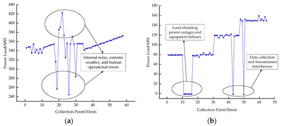
Figure 1.
Schematic of abnormal power load data. (a) Fluctuation anomaly; (b) extreme mutation anomaly.
Figure 1a presents the variable power load abnormality curve, which illustrates the extreme values of abnormal load data. This curve is disrupted by the occurrence of load peaks, valleys, or faults at specific moments or within brief intervals, resulting in a loss of similarity and periodicity. In contrast, Figure 1b depicts the abnormal curve of fluctuating power load, which is characterized by abnormal periodic fluctuations occurring over short timeframes, along with frequent variations that deviate from established normal load fluctuation patterns.
The fluctuating abnormal load curve is characterized by numerous burrs and frequent short-term fluctuations, which significantly deviate from the normal load fluctuation pattern. In contrast, the extreme abnormal load curve is characterized by extreme abnormal load data, where pronounced peaks, troughs, or substantial differences between peaks and troughs occur within a specific timeframe, typically lasting several minutes. This disruption reduces the similarity and periodicity of the curve. The abnormal characteristics and their corresponding causes of abnormal power load data are summarized in Table 1. Load data exhibiting abnormal fluctuations often stem from internal noise or external interference, particularly during extreme weather conditions or due to human operational errors. Conversely, data exhibiting extreme values and abnormalities typically arise from the loss of collected data at specific times, which may result from load shedding, power outages, or faults in equipment such as transformers, cables, and protection devices. Additionally, interference in data collection and transmission, as well as instances of user power theft, may also cause abnormalities. In the daily operations of most industries and electricity consumers, electricity peaks in the daily load curve are common when the most electricity-intensive equipment is utilized, leading to transitions between multiple production and operational states. This results in a higher probability of recurrence for the maximum load peak. Furthermore, special circumstances, such as holidays, may induce sudden changes in power demand, resulting in load abnormalities. In these cases, the power load data are typically considered to be in a normal state. However, when identifying abnormal power load data, the presence of these normal factors or characteristics may contribute to a certain rate of false detections.

Table 1.
Factors contributing to abnormal load data.
3. The Principles of One-Hot Encoding and the GAN–Transformer Model
3.1. One-Hot Encoding
In the field of data processing, categorical data are often represented in textual form. However, many algorithmic models, such as logistic regression and support vector machines, are unable to process these textual data; therefore, it is essential to convert them into numerical formats. One-hot encoding is not necessary when reasonable distance calculations can be made directly between categories [34].
One-hot encoding emerges as an effective solution to this issue. As a robust method for processing categorical data, it enhances the rationality of data during similarity or distance calculations and improves accuracy by transforming category values into One-hot vectors. This encoding strategy, also known as One-hot encoding, utilizes sparse vectors to represent each category, thereby circumventing the irrationalities that may arise from label encoding in distance calculations. In numerous machine learning tasks, particularly those involving non-numeric data, One-hot encoding serves as an effective data preprocessing strategy. In a typical logistic regression model, the expression for continuous variables is as follows:
where w is the weight of the continuous variable x.
When using One-hot encoding, the expression of the model is the following:
where are the components following One-hot encoding; and represent the weight associated with the components.
One-hot encoding transforms categorical variables into binary vectors, where each vector has a value of 1 at the corresponding integer index and 0 at all other positions, thereby creating a sparse representation. This method effectively avoids any ordinal relationships that might be inadvertently introduced by numerical values, making it particularly beneficial for categories that lack a natural order. The expression for one-hot encoding can be denoted as follows:
where i signifies the i-th eigenvalue, indicated by a value of 1 at that position. The dimensionality of this vector is determined by the number of distinct eigenvalues.
3.2. GAN–Transformer Model
3.2.1. Generator
The structure of the GAN–Transformer model, as illustrated in Figure 2, is employed. Generator 1 produces a reconstruction sequence that integrates abnormal focus scores and positional encoding features derived from the load data. By utilizing the Transformer generator architecture, the focus scores and positional encoding information are used as inputs, resulting in the reconstruction data of the input sequence . During the forward propagation process in Generator 1, the initial attention scores are represented as a zero vector and combined with positional encoding information , which serves as input to the multi-head attention layer. The output is denoted as . Next, and are processed through a residual connection and normalization layer, producing the output . The input then passes through a feed-forward network, followed by a second residual connection and normalization layer. After ReLU activation and linear transformation, along with the residual connection, the final output is obtained. Generator 1 can be expressed as follows:
where represents the multi-head attention operation applied to the concatenated input matrix ; refers to the feed-forward network operation applied to the input matrix ; and denotes the normalization process applied to the input values at each layer.

Figure 2.
GAN–Transformer model structure.
Generator 2 is employed to reconstruct the input power load sequence. During the forward propagation in Generator 2, the power load sequence is combined with positional encoding information as input, and is processed through the first multi-head attention layer, with the output denoted as . Subsequently, and are processed through the first residual connection and normalization layer, producing the output . Next, passes through the second multi-head attention layer, followed by another residual connection and normalization, yielding the output . Generator 2 can be represented as follows:
3.2.2. Discriminator
Discriminator 1 and Discriminator 2 are composed of a position feed-forward network followed by a Sigmoid activation function. The expressions for Discriminator 1 and Discriminator 2 in the first stage are provided by the following equations:
In the second stage, Discriminator 2 is defined by the following equation:
where represents the output of Discriminator 1 in the first stage; is the output of Discriminator 2 in the first stage; refers to the output of Discriminator 2 in the second stage; and denotes the activation function.
3.2.3. Staged Mapping and Training
The model employs a staged training strategy that includes multiple mappings to reconstruct the input power load sequence. For instance, in two-stage mapping, the output from the first stage is utilized as the input for the second stage.
First Stage: Model Mapping Phase
Generator 1: The initial attention scores, set as a zero vector, are combined with positional encoding information and input into Generator 1.
Discriminator 1: The outputs of both Generator 1 and Generator 2 are fed into Discriminator 1, which produces the reconstructed sequence .
Generator 2: Historical power load data are combined with positional encoding and input into Generator 2. The output of Generator 1 also serves as part of the input to the multi-head attention layer in Generator 2.
Discriminator 2: The output of Generator 2 is evaluated by Discriminator 2, yielding the reconstructed sequence .
Second Stage: Model Training and Remapping Phase
Adversarial Training: Based on the mappings from the first stage, the model undergoes adversarial training to refine the generators and discriminators.
Remapping: The reconstruction loss from Discriminator 1 during the first stage is used as the attention score for the subsequent second stage. After positional encoding, this score is reintroduced into Generator 1. Similarly, the reconstructed sequence from the first stage is reintroduced into Generator 2 after positional encoding.
Final Output: Discriminator 2′s output during this stage is the final reconstructed power load time-series sequence .
This multi-stage mapping approach, particularly the use of adversarial training and remapping, aims to enhance the accuracy and robustness of the reconstructed sequences.
3.2.4. Loss Function
The primary objective of the model in its initial stage is to generate a reconstruction sequence that aligns with the distribution of the input load data. By emphasizing the reconstruction loss results as the focal score, the generator is encouraged to concentrate on subsequences that exhibit abnormal trends.
The reconstruction loss functions for Discriminator 1 and Discriminator 2 during the first stage, and , are, respectively, defined as follows:
In the second stage, during model training and remapping, the reconstruction loss functions for Discriminator 1 and Discriminator 2 are defined as and , which are, respectively, defined as follows:
By combining the loss functions of Discriminator 1 and Discriminator 2 during the first and second stages, we derive the overall loss functions and for the model, as detailed in the following equations:
where n represents the number of training iterations, while ε denotes hyperparameters that typically assume values close to 1.
4. Implementation of Abnormal Detection and Classification of Power Load Data
4.1. Exception Type Annotation Implementation
One-hot encoding is applied in both the discrete feature classification process and the model’s feature mapping process to prepare suitable input data for the GAN–Transformer model.
This paper classifies the characteristics of abnormal load data based on the waveform expression and the distinctive data features. As shown in Table 2, four types of abnormal loads are identified. Abnormal load data characterized by waveforms exhibiting spikes are defined as mutation anomalies. These mutation anomalies typically arise in scenarios involving impact loads and signal interference. This category of abnormal load data is encoded as 0001 using One-hot encoding. Conversely, abnormal load data that present long-term extreme values in their waveforms are classified as long-term extreme value anomalies. Such data generally occur in contexts such as acquisition failures, equipment maintenance, line failures, and power plant accidents, and are represented as 0010 in One-hot encoding. Additionally, abnormal load data that display a fluctuating waveform are categorized as fluctuating anomalies, which are often associated with noise interference. These types of data are encoded as 0100 using One-hot encoding. Finally, abnormal load data characterized by short-term extreme values in their waveforms are defined as short-term extreme value anomalies. This category typically arises in scenarios such as load-shedding power outages and SCADA temporary failures, and it is represented as 1000 in One-hot encoding.

Table 2.
Types of abnormal loads and One-hot encoding.
4.2. Implementation Process
The pseudocode of the power load anomaly detection and classification system is shown in Table 3.

Table 3.
Pseudocode of anomaly detection and classification.
- (1)
- Data Preprocessing: The collected historical power load data are first divided into training and test sets in a 7:3 ratio. Missing values are addressed through standard procedures, and the data are normalized to ensure uniformity.
- (2)
- Label Processing: To capture the diverse characteristics of abnormal load data, One-hot encoding is applied to label the anomaly types. These labeled data are then prepared as inputs and outputs for model training.
- (3)
- Model Training: The GAN–Transformer model is trained on a substantial volume of labeled abnormal load data. Throughout the training process, hyperparameters are iteratively adjusted. The training spans 500 epochs, with early stopping implemented if the training loss does not improve for 10 consecutive epochs. The weights of the best-performing model are saved for subsequent testing.
- (4)
- Model Testing and Analysis: The saved model is loaded to predict anomalies in the test set. The model generates detection results, identifying anomalies, as well as classification results that categorize the types of anomalies. Finally, metrics such as accuracy, precision, recall, and F1-score are calculated to evaluate performance, followed by a comprehensive analysis of the results.
4.3. Abnormal Load Data Detection Mechanism
To accurately identify anomalies in the input load data, the data are compared with the reconstructed sequence generated in the first stage of the model. An anomaly score and an anomaly diagnosis label are introduced for the purpose of anomaly detection.
The anomaly score is defined as the sum of the L2 norms between the reconstructed sequences from the two stages and the input data. A higher anomaly score indicates a greater deviation in the load data at that specific point. The anomaly diagnosis label is determined based on the anomaly score at a given time point, where a time point is considered anomalous if its anomaly score exceeds a predefined threshold.
The Peaks Over Threshold (POT) method is employed to automatically and dynamically select the threshold.
The anomaly score and anomaly diagnosis label are denoted as s and y.
where is the anomaly score; and is the threshold set using the Peaks Over Threshold (POT) method. is the anomaly diagnosis label, where indicates that the data at time t are anomalous, and indicates that the data at time t are normal.
4.4. Model Performance Evaluation Indicators
Precision, recall, and F1-score are used to comprehensively evaluate the anomaly detection performance of the GAN–Transformer model.
where (True Positives) represents the number of correctly detected abnormal samples (prediction: 1; ground truth: 1). (False Positives) refers to the number of samples incorrectly identified as anomalies when they are actually normal (prediction: 1; ground truth: 0). (False Negatives) denotes the number of abnormal samples that were not detected (prediction: 0; ground truth: 1). Additionally, precision () and recall () are used as key metrics to evaluate detection performance.
Three commonly used indicators for evaluating model classification performance are OA, AA, and the Kappa coefficient. OA measures the proportion of correct classifications made by the model among all test samples, serving as the most intuitive performance indicator. AA takes into account the accuracy of each category and calculates its average, thereby mitigating evaluation bias that may arise from category imbalance. The Kappa coefficient quantifies the difference between the actual accuracy of the classification outcomes and the accuracy expected from random classification. A larger Kappa value indicates superior performance of the classification model.
where represents the number of correctly classified samples, and denotes the total number of samples. C indicates the total number of abnormal load types, is the number of correctly classified samples in the i-th abnormal load type, and represents the total number of samples in the i-th abnormal load type. The Kappa value ranges from −1 to 1, where Kappa > 0.8 indicates “excellent” agreement; Kappa 0.6–0.8 indicates “good” agreement; Kappa 0.4–0.6 indicates “fair” agreement; and Kappa < 0.4 indicates “poor agreement”.
The definition of in Equation (14) is the accidental consistency error, which can be expressed as follows:
where represents the number of real samples of the i-th category in the load feature category, and represents the number of predicted samples of the i-th category in the load feature category.
5. Experimental Research and Discussion
5.1. Experimental Preparation
The load dataset is normalized using the min–max normalization method, which scales both the input training sample data and the output power load reconstruction data to dimensionless values within the range of [0, 1].
where min and max are the vectors representing the minimum and maximum values in the time-series, respectively; is a constant vector; and is the normalized value of the training sample data at time t.
To evaluate the effectiveness of the GAN–Transformer model utilizing One-hot annotation for classifying anomalies in power load data, an experimental environment was established using the Python 3.8 interpreter and the PyCharm 2022.2 development environment, running on Intel Core i7-13700 (CA, USA) and NVIDIA RTX4060 (CA, USA) with Kingston 32 GB of RAM (USA), under the Windows 10 operating system. The dataset used is consistent with the one employed in the power load data anomaly detection study discussed in this paper. Data were collected at 30 s intervals over a span of 90 days. The dataset was randomly partitioned into a training set and a test set in a 7:3 ratio, with the classification results illustrated in Figure 3. The hyperparameter values are shown in Table 4.
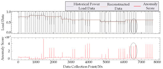
Figure 3.
Detection results for abnormal supply load data.

Table 4.
Hyperparameter settings of GAN–Transformer model.
5.2. Detection of Abnormal Load Data in Power Supply and Consumption
In Figure 3 and Figure 4, the horizontal axis represents power load data sampled at 30 s intervals, while the vertical axis displays the normalized reconstruction output (ranging from 0 to 1) and anomaly diagnosis scores from the GAN–Transformer model. Gray shaded areas highlight regions with potential load anomalies. The anomaly score curve, composed of POT values, identifies anomalies where scores exceed the threshold, with higher bar amplitudes signifying greater anomaly severity.
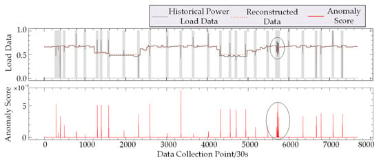
Figure 4.
Detection results for abnormal consumption load data.
Figure 5a,b are magnified views of the circled regions in Figure 3 and Figure 4, respectively, presenting zoomed-in views of historical and reconstructed load data and detailing the detection results for fluctuation anomalies. In these figures, the reconstructed data generated by Discriminator 2 effectively captures the variation characteristics of the power load curves. The comparison between historical data and reconstructed sequences, along with the anomaly score results, demonstrate that the GAN–Transformer model accurately detects and identifies extreme value and fluctuation anomalies in the load data.
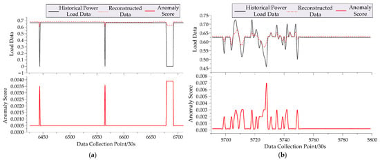
Figure 5.
Details of anomaly detection results. (a) Power supply load data; (b) power consumption load data.
To ensure the validity of the simulation results and to provide a clear observation of the GAN–Transformer model, the decrease in loss values during model training is illustrated in Figure 6a,b. The analysis of Figure 6 reveals that the model demonstrates effective training performance for both power supply and consumption load anomaly detection across the training and testing sets. With the total number of training epochs set at 500, the loss values reach their minimum between the 30th and 40th epochs, indicating that the model achieves a well-fitted state at this stage.
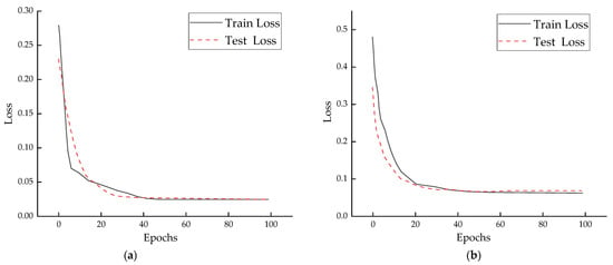
Figure 6.
Training and testing performance of anomaly detection. (a) Power supply load data; (b) power consumption load data.
5.3. Classification of Abnormal Load Data in Power Supply and Consumption
The abscissas in Figure 7 and Figure 8 represent the power load data collected at equal intervals, while the ordinates illustrate the reconstructed output and the classification results of abnormal data after normalizing the power load data using the GAN–Transformer model within the interval [0, 1]. The black solid line denotes the historical power supply load data to be detected, the red dotted line indicates the model’s reconstruction results, and the blue solid line represents the classification results for abnormal data.
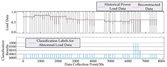
Figure 7.
Classification results for abnormal supply load data.
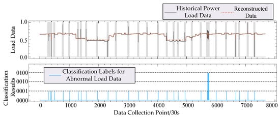
Figure 8.
Classification results for abnormal consumption load data.
Figure 9a presents a pie chart that illustrates the classification results of abnormal power supply load data following model training. The chart shows that in the experimental power supply load data, the load data labeled as 0001 constitute 73.3% of the total abnormal load data. In contrast, the load data classified as 0010 account for 21.7%, while the load data marked as 1000 represent 5% of the abnormal load data. These results indicate a clear and well-defined classification distribution of the abnormal load data based on feature information, thereby highlighting the model’s effective performance.
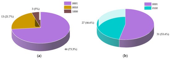
Figure 9.
Pie chart of abnormal load data classification results. (a) Supply load data; (b) consumption load data.
Figure 9b presents a pie chart illustrating the classification results of abnormal load data following model training. The chart indicates that, within the experimental dataset, the load data categorized as abnormal and labeled 0001 constitute 53.4% of the total abnormal load data. In contrast, the load data corresponding to abnormal conditions, labeled 0100, account for 46.6% of the detected abnormal load data. Following model training, the abnormal load data are effectively classified into two distinct types of feature information, resulting in a clearer and more defined feature distribution.
5.4. Comparative Analysis of Algorithms
To validate the superiority of the One-hot labeled GAN–Transformer model for abnormal load data detection, comparative experiments were conducted with LSTM-NDT, Transformer, OmniAnomaly and MAD-GAN as baseline models. All models were trained for 500 epochs. The results of the anomaly detection for both power supply load data and power consumption load data across the various models are presented in Table 5 and Table 6, respectively.

Table 5.
Experimental results of supply load data detection using different models.

Table 6.
Experimental results of consumption load data detection using different models.
The analysis of anomaly detection results for power supply load data, as presented in Table 5, demonstrates that the GAN–Transformer model achieves a detection precision of 0.9492, reflecting a 10% to 20% improvement over the baseline models. However, its recall rate is 0.9384, which is slightly lower than that of the comparison models, indicating a reduced detection coverage for anomalies. This observation suggests that the model may have a lower false alarm rate.
In the context of power load data detection and identification, Table 6 demonstrates that the GAN–Transformer model exhibits a notable advantage, achieving a detection precision of 0.9762. Meanwhile, its recall rate is 0.9264, which is comparable to that of the other models.
When considering both precision and recall, the GAN–Transformer model achieves an F1-score of 0.9437 in Table 5 and 0.9506 in Table 6, both significantly higher than those of the baseline models and approaching the ideal value of 1.
Furthermore, an analysis of training efficiency indicates that, with the same number of training iterations, the GAN–Transformer model achieves a 70% reduction in training time while significantly enhancing anomaly detection accuracy. This highlights its superior overall performance.
To ensure a fair comparison, all models were trained and tested using the same dataset. As demonstrated in Table 7 and Table 8, the proposed model outperforms LSTM-NDT, Transformer, OmniAnomaly, and MAD-GAN in classifying anomalies in both supply and consumption load across all evaluation metrics.

Table 7.
Experimental results of supply load data classification using different models.

Table 8.
Experimental results of consumption load data classification using different power models.
In this study, Overall Accuracy (OOA) and Average Accuracy (AAA) are utilized as key evaluation metrics. OOA reflects the overall classification accuracy and is suitable for datasets with balanced class distributions, while AAA calculates the average classification accuracy across all classes, making it more appropriate for imbalanced datasets and providing a fairer evaluation of the model’s performance across different classes. Additionally, the Kappa coefficient is employed to measure the consistency between the classification results and random chance, thereby mitigating the impact of data imbalance. Typically, a Kappa value between 0.6 and 0.8 indicates good consistency, while a Kappa value above 0.8 indicates a high level of reliability.
Specifically, the proposed model achieves the highest scores in OOA, AAA, and KKappa. Compared to LSTM-NDT, OOA improved by 3.27–18.67%, AAA increased by 2.86–14.51%, and KKappa rose by 0.0987–0.2849. Compared to Transformer, OOA improved by 3.49–5.19%, AAA increased by 0.4–3.81%, and KKappa rose by 0.0887–0.0944. Moreover, the proposed method outperforms OmniAnomaly and MAD-GAN, with OOA improving by up to 5.47% and 2.97%, respectively, further validating its effectiveness. In summary, the method presented in this article demonstrates superior accuracy in load anomaly classification when compared to both LSTM-NDT and Transformer models. This indicates that the load anomaly classification approach utilized in this study effectively integrates the strengths of the attention mechanism and One-hot encoding, thereby enhancing the accuracy of abnormal load data classification.
The results demonstrate that the proposed method effectively integrates the attention mechanism and One-hot encoding, achieving optimal results in OOA, AAA, and KKappa. With a Kappa coefficient exceeding 0.8, the model’s classification results are highly reliable, further confirming the robustness and effectiveness of the method for complex load anomaly detection tasks.
6. Conclusions
In this paper, we propose an enhanced GAN–Transformer model within the GAN framework, providing a detailed description of the architecture, generator, discriminator, and mathematical expressions for the loss function. The feature mapping and training process are structured into two stages, with the output from the first stage serving as the input for the second stage. This methodology improves the model’s capacity to capture the trend change characteristics of power load data in the reconstructed load sequences. Furthermore, we introduce a focus score mechanism to facilitate anomaly detection in load data. The implementation of One-hot encoding ensures the accurate classification of categorical anomaly types, thereby enhancing both the interpretability and accuracy of the model.
Experimental results demonstrate that the proposed model significantly outperforms traditional models such as OmniAnomaly, MAD-GAN, LSTM-NDT, and Transformer, achieving higher precision, recall, and F1-score in detection, higher accuracy, and a better Kappa coefficient in classification. The model effectively detects various anomalies, including mutation anomalies, sustained extreme anomalies, spike anomalies, and transient extreme anomalies, which are common in real-world power load datasets. However, there are still areas for future improvement. While the model performs excellently on the datasets used in this study, further research is needed to explore its adaptability to more diverse and large-scale datasets, including those with different distributions, higher levels of noise, or incomplete data. Additionally, although the current implementation achieves satisfactory accuracy, its computational complexity could be further reduced to enhance scalability in resource-constrained environments, such as real-time anomaly detection for operational power systems. Moreover, optimizing the model’s efficiency would better support predictive maintenance tasks requiring rapid response capabilities.
Author Contributions
Conceptualization, T.Y.; software, H.Y.; validation, W.F.; formal analysis, D.L. and S.B.; writing—original draft, H.Y.; writing—review and editing, Y.L.; supervision, K.L. All authors have read and agreed to the published version of the manuscript.
Funding
This research was funded by the Natural Science Foundation of Jiangsu Province (No. BK20210932).
Data Availability Statement
The original contributions presented in this study are included in this article. Further inquiries can be directed to the corresponding author.
Conflicts of Interest
The authors declare no conflicts of interest.
References
- Klein, M.; Thiele, G.; Fono, A.; Khorsandi, N.; Schade, D.; Krüger, J. Process data based Anomaly detection in distributed energy generation using Neural Networks. In Proceedings of the 2020 International Conference on Control, Automation and Diagnosis (ICCAD), Paris, France, 7–9 October 2020; pp. 1–5. [Google Scholar]
- Kwasinski, A. Quantitative model and metrics of electrical grids’ resilience evaluated at a power distribution level. Energies 2016, 9, 93. [Google Scholar] [CrossRef]
- Deng, S.; Chen, F.; Dong, X.; Gao, G.; Wu, X. Short-term load forecasting by using improved GEP and abnormal load recognition. ACM Trans. Internet Technol. (TOIT) 2021, 21, 1–28. [Google Scholar] [CrossRef]
- Tianhui, Z.; Zhang, Y.; Jianxue, W. Identification method of load outlier based on density-based spatial clustering and outlier boundaries. Autom. Electr. Power Syst. 2021, 45, 97–105. [Google Scholar]
- Chandola, V.; Banerjee, A.; Kumar, V. Anomaly detection: A survey. ACM Comput. Surv. (CSUR) 2009, 41, 1–58. [Google Scholar] [CrossRef]
- Wang, H.; Bah, M.J.; Hammad, M. Progress in outlier detection techniques: A survey. IEEE Access 2019, 7, 107964–108000. [Google Scholar] [CrossRef]
- Shen, X.; Luo, Z.; Li, Y.; Ouyang, T.; Wu, Y. Chance-Constrained Abnormal Data Cleaning for Robust Classification with Noisy Labels. IEEE Trans. Emerg. Top. Comput. Intell. 2024, 1–8. [Google Scholar] [CrossRef]
- Saeed, M.S.; Mustafa, M.W.; Sheikh, U.U.; Jumani, T.A.; Mirjat, N.H. Ensemble bagged tree based classification for reducing non-technical losses in multan electric power company of Pakistan. Electronics 2019, 8, 860. [Google Scholar] [CrossRef]
- He, Y.; Ma, Y.; Huang, K.; Wang, L.; Zhang, J. Abnormal data detection and recovery of sensors network based on spatiotemporal deep learning methodology. Measurement 2024, 228, 114368. [Google Scholar] [CrossRef]
- Luo, Z.; Fang, C.; Liu, C.; Liu, S. Method for cleaning abnormal data of wind turbine power curve based on density clustering and boundary extraction. IEEE Trans. Sustain. Energy 2021, 13, 1147–1159. [Google Scholar] [CrossRef]
- Tran-Nam, H.; Nguyen-Trang, T.; Che-Ngoc, H. A new possibilistic-based clustering method for probability density functions and its application to detecting abnormal elements. Sci. Rep. 2024, 14, 17871. [Google Scholar] [CrossRef]
- Liang, G.; Liao, H.; Huang, Z.; Li, X. Abnormal discharge detection using adaptive neuro-fuzzy inference method with probability density-based feature and modified subtractive clustering. Neurocomputing 2023, 551, 126513. [Google Scholar] [CrossRef]
- Li, J.; Izakian, H.; Pedrycz, W.; Jamal, I. Clustering-based anomaly detection in multivariate time series data. Appl. Soft Comput. 2021, 100, 106919. [Google Scholar] [CrossRef]
- Li, C.; Guo, L.; Gao, H.; Li, Y. Similarity-measured isolation forest: Anomaly detection method for machine monitoring data. IEEE Trans. Instrum. Meas. 2021, 70, 1–12. [Google Scholar] [CrossRef]
- Peng, Y.; Yang, Y.; Xu, Y.; Xue, Y.; Song, R.; Kang, J.; Zhao, H. Electricity theft detection in AMI based on clustering and local outlier factor. IEEE Access 2021, 9, 107250–107259. [Google Scholar] [CrossRef]
- Liu, X.; Ding, Y.; Tang, H.; Xiao, F. A data mining-based framework for the identification of daily electricity usage patterns and anomaly detection in building electricity consumption data. Energy Build. 2021, 231, 110601. [Google Scholar] [CrossRef]
- Qian, Y.; Wang, Y.; Shao, J. Enhancing power utilization analysis: Detecting aberrant patterns of electricity consumption. Electr. Eng. 2024, 106, 5639–5654. [Google Scholar] [CrossRef]
- Lei, X.; Xia, Y.; Wang, A.; Jian, X.; Zhong, H.; Sun, L. Mutual information based anomaly detection of monitoring data with attention mechanism and residual learning. Mech. Syst. Signal Process. 2023, 182, 109607. [Google Scholar] [CrossRef]
- Yang, N.-C.; Sung, K.-L. Non-intrusive load classification and recognition using soft-voting ensemble learning algorithm with decision tree, K-Nearest neighbor algorithm and multilayer perceptron. IEEE Access 2023, 11, 94506–94520. [Google Scholar] [CrossRef]
- Cai, Q.; Li, P.; Wang, R. Electricity theft detection based on hybrid random forest and weighted support vector data description. Int. J. Electr. Power Energy Syst. 2023, 153, 109283. [Google Scholar] [CrossRef]
- Choi, J.; Roshanzadeh, B.; Martínez-Ramón, M.; Bidram, A. An unsupervised cyberattack detection scheme for AC microgrids using Gaussian process regression and one-class support vector machine anomaly detection. IET Renew. Power Gener. 2023, 17, 2113–2123. [Google Scholar] [CrossRef]
- Shahid, S.M.; Ko, S.; Kwon, S. Real-time abnormality detection and classification in diesel engine operations with convolutional neural network. Expert Syst. Appl. 2022, 192, 116233. [Google Scholar] [CrossRef]
- Zamanzadeh Darban, Z.; Webb, G.I.; Pan, S.; Aggarwal, C.; Salehi, M. Deep learning for time series anomaly detection: A survey. ACM Comput. Surv. 2024, 57, 1–42. [Google Scholar] [CrossRef]
- Kumari, S.; Prabha, C.; Karim, A.; Hassan, M.M.; Azam, S. A Comprehensive Investigation of Anomaly Detection Methods in Deep Learning and Machine Learning: 2019–2023. IET Inf. Secur. 2024, 2024, 8821891. [Google Scholar] [CrossRef]
- Lei, C.; Kai, Q.; Kuangrong, H. Time series anomaly detection method based on integrated LSTM-AE. J. Huazhong Univ. Sci. Technol. (Nat. Sci. Ed.) 2021, 49, 35–40. [Google Scholar]
- Su, Y.; Zhao, Y.; Niu, C.; Liu, R.; Sun, W.; Pei, D. Robust anomaly detection for multivariate time series through stochastic recurrent neural network. In Proceedings of the 25th ACM SIGKDD International Conference on Knowledge Discovery & Data Mining, Anchorage, AK, USA, 4–8 August 2019; pp. 2828–2837. [Google Scholar]
- Li, J.; Lv, Y.; Zhou, Z.; Du, Z.; Wei, Q.; Xu, K. Identification and Correction of Abnormal, Incomplete Power Load Data in Electricity Spot Market Databases. Energies 2025, 18, 176. [Google Scholar] [CrossRef]
- Li, D.; Chen, D.; Jin, B.; Shi, L.; Goh, J.; Ng, S.-K. MAD-GAN: Multivariate anomaly detection for time series data with generative adversarial networks. In Proceedings of the International Conference on Artificial Neural Networks, Munich, Germany, 17–19 September 2019; pp. 703–716. [Google Scholar]
- Yang, Z.; Zhang, W.; Cui, W.; Gao, L.; Chen, Y.; Wei, Q.; Liu, L. Abnormal detection for running state of linear motor feeding system based on deep neural networks. Energies 2022, 15, 5671. [Google Scholar] [CrossRef]
- Feng, C.; Shao, L.; Wang, J.; Zhang, Y.; Wen, F. Short-term Load Forecasting of Distribution Transformer Supply Zones Based on Federated Model-Agnostic Meta Learning. IEEE Trans. Power Syst. 2024, 40, 31–45. [Google Scholar] [CrossRef]
- Xu, J. Anomaly transformer: Time series anomaly detection with association discrepancy. arXiv 2021, arXiv:2110.02642. [Google Scholar]
- Wang, L.; Wang, X.; Zhang, J.; Wang, J.; Yu, H. A self-supervised learning-based approach for detection and classification of dam deformation monitoring abnormal data with imaging time series. Structures 2024, 68, 107148. [Google Scholar] [CrossRef]
- Shi, J.; Gao, Y.; Gu, D.; Li, Y.; Chen, K. A novel approach to detect electricity theft based on conv-attentional Transformer Neural Network. Int. J. Electr. Power Energy Syst. 2023, 145, 108642. [Google Scholar] [CrossRef]
- Poslavskaya, E.; Korolev, A. Encoding categorical data: Is there yet anything ‘hotter’ than one-hot encoding? arXiv 2023, arXiv:2312.16930. [Google Scholar]
Disclaimer/Publisher’s Note: The statements, opinions and data contained in all publications are solely those of the individual author(s) and contributor(s) and not of MDPI and/or the editor(s). MDPI and/or the editor(s) disclaim responsibility for any injury to people or property resulting from any ideas, methods, instructions or products referred to in the content. |
© 2025 by the authors. Licensee MDPI, Basel, Switzerland. This article is an open access article distributed under the terms and conditions of the Creative Commons Attribution (CC BY) license (https://creativecommons.org/licenses/by/4.0/).