Review of Data-Driven Approaches Applied to Time-Series Solar Irradiance Forecasting for Future Energy Networks

Abstract

The fast-increasing penetration of photovoltaic (PV) power raises the issue of grid stability due to its intermittency and lack of inertia in power systems. Solar irradiance forecasting effectively supports advanced control, mitigates power intermittency, and improves grid resilience. Irradiance forecasting based on data-driven methods aims to predict the direction and level of power variation and indicate quick action. This article presents a comprehensive review and comparative analysis of data-driven approaches for time-series solar irradiance forecasting. It systematically evaluates nineteen representative models spanning from traditional statistical methods to state-of-the-art deep learning architectures across multiple performance dimensions that are critical for practical deployment. The analysis aims to provide actionable insights for researchers and practitioners when selecting and implementing suitable forecasting solutions for diverse solar energy applications.

1. Introduction

Photovoltaic (PV) solar power generation is a promising, sustainable, and renewable technology for future energy networks [1,2]. Solar generation comes from natural sunlight, which can rapidly vary under environmental conditions, e.g., moving clouds [3]. Fast growth leads to a high penetration of PV energy into the existing power system, raising concerns about grid instability and presenting new challenges [4,5]. These integration challenges parallel those faced by other renewable and sustainable technologies, such as electric vehicles, which similarly require sophisticated forecasting and management strategies to maintain grid stability while achieving carbon reduction objectives [6]. A stable operation of the grid network depends on the balance between the generation and demand sides. However, intermittent solar power generation can cause an imbalance that will result in a potential malfunction in the regulation of voltage and frequency [7,8].

Power ramp rate control (PRRC) is a strategy that can mitigate intermittent power and support smooth power output of PV systems and minimize the negative impact on grid stability [9,10]. To achieve PRRC, one solution relies on energy storage systems (ESSs) as the energy buffer and mimics the mechanical inertia provided by the spinning mass of traditional turbine generators [11]. However, the ESS approach is considered a simple but expensive solution due to the high price and life span of batteries [12]. Thus, the latest research focuses on time-series solar irradiance forecasting (TSSIF) and provides a cost-effective solution to support the PRRC for grid resilience [13,14].

1.1. Time-Series Solar Irradiance Forecasting

Data-driven approaches for TSSIF formulate the problem as statistical prediction of future irradiance values, denoted $X_t$, which is conditioned on a historical sequence of observed irradiance values $X_{t-1};X_{t-2};\dots ;X_{t-n+1};X_{t-n}$ [15,16]. For some models, they can accept additional exogenous variables (e.g., satellite-derived cloud indices, temperature, humidity, temporal feature) $X_{t-n}=\left\{x_{t-n}^{\left(1\right)},x_{t-n}^{\left(2\right)},\dots ,x_{t-n}^{\left(k\right)}\right\}$ to further improve the prediction performance [17,18]. The core objective is to learn a functional mapping from historical information to future targeted data, as shown in Figure 1.

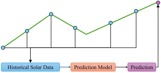
Figure 1. A depiction of typical time-series solar irradiance forecasting systems.

1.2. Classification

In recent decades, considerable research efforts have focused on developing accurate and reliable TSSIF [19]. It establishes a fundamental framework for capturing linear temporal dependencies and trend patterns, classified into two main categories: traditional statistical models and modern machine learning approaches, [20,21]. Traditional statistical methods, e.g., autoregressive (AR) and moving average (MA) are computationally efficient and interpretable, struggling to handle the inherent nonlinearity and complex patterns in solar irradiance data that are caused by atmospheric dynamics and cloud behaviors [22].

The emergence of machine learning has significantly revolutionized solar forecasting capabilities [23]. Deep learning architectures, particularly recurrent neural networks (RNNs) and long short-term memory (LSTM) networks, have shown superior performance in capturing long-term dependencies and nonlinear relationships [24,25]. More recently, advanced architectures such as convolutional neural networks (CNNs) for extracting spatial features from satellite images [26], graph neural networks (GNNs) for distributed sensor network applications [27], and transformer models with attention mechanisms have further pushed the limits of prediction accuracy [28,29]. Hybrid models that combine multiple architectures have emerged as especially promising solutions, which leverage complementary strengths to address the multiscale spatio-temporal characteristics of solar irradiance variability [30,31].

Despite these advances, selecting an appropriate forecasting model remains challenging due to trade-offs between accuracy, computational burden, data requirements, and operational constraints [32]. Different applications—ranging from real-time grid control to day-ahead energy trading—require varying prediction horizons and performance characteristics [33]. Furthermore, practical deployment considerations including available historical data, computational resources, and robustness against extreme weather events, can significantly influence the model selection process [34,35].

This paper provides a comprehensive technical review of data-driven approaches for time-series solar irradiance forecasting, focusing on algorithmic characteristics, mathematical formulations, and theoretical performance comparisons. While it systematically evaluates computational complexity, accuracy metrics, and data requirements, practical engineering deployment involves additional considerations beyond our current scope. The technical analysis provides the foundational understanding necessary for researchers and practitioners to evaluate these models, with the recognition that deployment decisions must also account for site-specific engineering constraints and operational requirements. The remainder of this paper is organized as follows. Section 2 reviews classical statistical models and explains their theoretical foundations and solar forecasting applications. Section 3 explores machine learning and deep learning approaches, showing a detailed analysis of their mechanisms and advantages. Section 4 presents a systematic comparative study evaluating all models regarding computational complexity, accuracy, data requirements, robustness, and application scenarios specific to solar irradiance forecasting. Finally, Section 5 concludes the paper with key findings and future research directions.

2. Classical Methods Based on Statistical Models

Traditional statistical methods have been applied to solar irradiance prediction for a long time, with the earliest work traced back to 1977 when researchers used stochastic models for forecasting [36]. These statistical models remain foundational due to their interpretability, solid theoretical basis, and often excellent performance, particularly when domain knowledge is effectively incorporated [37,38]. While machine learning models are becoming increasingly popular, statistical approaches are typically the first approach to consider and frequently establish the benchmark for comparison [39].

2.1. Autoregressive Model

Autoregressive (AR) models have emerged as fundamental tools for early solar irradiance forecasting, which operate on the principle that future values can be predicted as a weighted linear combination of past observations. The AR(p) model can be defined as:

$$X_t=c+\sum _{i=1}^p{\varphi }_i{X}_{t-i}+{\epsilon }_t$$

(1)

$X_t:$

Value of the time series at time t;

c: 

Constant (intercept) term;

p: 

Order of the autoregression (number of lags);

${\varphi }_i:$

Autoregressive coefficients;

$X_{t-i}:$

Lag-i observation;

${\epsilon }_t:$

White noise error term at time t with $\mathbb{E}\left[{\epsilon }_t\right]=0$, $\mathrm{Var}\left({\epsilon }_t\right)={\sigma }^2$.

This approach can capture short-term persistence during a clear-sky period but neglects critical exogenous factors such as cloud movement patterns [40].

2.2. Moving-Average Model

Moving-average (MA) models complement AR models by incorporating past forecast errors (residuals), which improves the responsiveness to abrupt changes. Nevertheless, both models fundamentally assume stationarity—requiring constant statistical properties over time—which directly contradicts the inherent diurnal cycles, seasonal trends, and weather-driven volatility of solar irradiance. During partly cloudy conditions, their errors can become significant, revealing severe limitations for practical deployment. The MA(q) model is expressed as:

$$X_t=\mu +{\epsilon }_t+\sum _{i=1}^p{\theta }_i{\epsilon }_{t-i}$$

(2)

$\mu :$

Mean of the time series ($\mathbb{E}\left[X_t\right]=\mu$);

${\theta }_i:$

Moving-average coefficient.

2.3. Autoregressive–Moving-Average Model

Autoregressive–moving average (ARMA) unifies AR and MA into a single framework where autoregressive lags capture persistent trends while moving-average terms adjust for recent errors. This hybrid approach can better model local irradiance dynamics compared to standalone AR or MA methods. The ARMA(p, q) model can be written as:

$$X_t=c+\sum _{i=1}^p{\varphi }_i{X}_{t-i}+{\epsilon }_t+\sum _{j=1}^q{\theta }_j{\epsilon }_{t-j}$$

(3)

where p and q denote the order of autoregressive (AR) and moving-average (MA) parts, respectively.

By dynamically balancing historical patterns and residual corrections, ARMA improves robustness against short-term noise [41]. However, it still retains the stationarity constraint, making it unable to handle systematic diurnal patterns or seasonal shifts. The strong daily periodicity of solar data (e.g., daily solar noon peaks) violates this assumption, which causes significant phase errors in multi-hour forecasts and requires manual de-trending procedures [42].

2.4. Autoregressive Integrated Moving-Average Model

Autoregressive integrated moving average (ARIMA) directly addresses the non-stationarity issue through differencing (integration). By transforming the original series into different terms, it removes trends and stabilizes variance. The ARIMA(p, d, q) model, which extends ARMA to non-stationary series by incorporating differencing, can be expressed as:

$${(1-L)}^d{X}_t=c+\sum _{i=1}^p{\varphi }_i{(1-L)}^d{X}_{t-i}+{\epsilon }_t+\sum _{j=1}^q{\theta }_j{\epsilon }_{t-j}$$

(4)

d: 

Order of differencing;

L: 

Lag operator ($L^k{X}_t=X_{t-k}$);

$X_t:$

Original time series value at time t.

A seasonal ARIMA (SARIMA) variant further incorporates periodic differencing to handle diurnal cycles, which can reduce forecasting errors in certain specific scenarios [43]. However, the differencing process erases nuanced temporal patterns, and the model remains inherently linear. More importantly, it cannot capture volatility clustering—the phenomenon where cloud-induced irradiance swings exhibit persistent high-variance periods followed by stable intervals. This leads to systematic underestimation of forecast uncertainty during variable weather conditions.

2.5. Autoregressive Conditional Heteroskedasticity Model

Autoregressive Conditional Heteroskedasticity (ARCH) revolutionizes volatility modeling by treating variance as time-dependent. ARCH with conditional variance directly links volatility to past squared residuals. The ARCH(q) model is defined by:

$$X_t=\mu +{\epsilon }_t$$

(5)

with conditional variance:

$${\sigma }_t^2={\alpha }_0+\sum _{i=1}^q{\alpha }_i{\epsilon }_{t-i}^2$$

(6)

where ${\epsilon }_t={\sigma }_t{\eta }_t$ and ${\eta }_t\sim \mathrm{i}.\mathrm{i}.\mathrm{d}.(0,1)$.

$X_t:$

Observed value at time t;

$\mu :$

Constant mean of $X_t$;

${\epsilon }_t:$

Residual error at time t;

${\sigma }_t^2:$

Conditional variance;

${\eta }_t:$

Standardized shock with $\mathbb{E}\left[{\eta }_t\right]=0$, $\mathrm{Var}\left({\eta }_t\right)=1$;

${\alpha }_0:$

Constant term (${\alpha }_0>0$);

${\alpha }_i:$

ARCH coefficient for lag i (${\alpha }_i\ge 0$);

q: 

Order of ARCH terms;

${\epsilon }_{t-i}^2:$

Squared residual at lag i.

A variant, Generalized Autoregressive Conditional Heteroskedasticity (GARCH), further generalizes this by including autoregressive variance terms. This explicitly models volatility clustering during intermittent cloud cover, where a large irradiance drop (e.g., from cumulus cloud passage) increases the predicted variance for subsequent timesteps. The experimental results show that GARCH reduces the prediction intervals compared to ARIMA in partly cloudy conditions [44]. Despite this improvement, both models assume linear relationships between residuals and variance, failing during nonlinear events such as thunderstorms or fog banks, where irradiance collapses follow asymmetric physical processes.

2.6. Vector Autoregression Model

Vector Autoregression (VAR) introduces multivariate modeling, treating irradiance and k exogenous variables (e.g., temperature, humidity, cloud cover indices) as endogenous components within a system of equations:

$$X_{j,t}=c_j+\sum _{i=1}^p{\varphi }_{j1}^{\left(i\right)}{X}_{1,t-i}+\sum _{i=1}^p{\varphi }_{j2}^{\left(i\right)}{X}_{2,t-i}+\dots +\sum _{i=1}^p{\varphi }_{jk}^{\left(i\right)}{X}_{k,t-i}+{\epsilon }_{j,t}$$

(7)

for each variable $j=1,2,\dots ,k$.

$X_{j,t}:$

Value of the j-th variable at time t ($j\in \{1,2,\dots ,k\}$).

$X_{1,t}:$

Solar irradiance at time t (primary variable, W/m²).

$X_{2,t},\dots ,X_{k,t}:$

Exogenous variables (temperature, humidity, pressure, etc.).

$c_j:$

Intercept term for the j-th equation (constant).

p: 

Order of VAR model (number of lagged observations used).

${\varphi }_{jl}^{\left(i\right)}:$

Coefficient matrix element, effect of variable l at lag i on variable j.

$X_{l,t-i}:$

Value of l-th variable at time $(t-i)$, lag $i\in \{1,\dots ,p\}$.

${\epsilon }_{j,t}:$

White noise error for j-th variable, $\mathbb{E}\left[{\epsilon }_{j,t}\right]=0$, $\mathrm{Var}\left({\epsilon }_{j,t}\right)={\sigma }_j^2$.

k: 

Total number of variables in the system.

This model can capture cross-correlations among multiple time-series data. For instance, increasing humidity may indicate the formation of stratus clouds and subsequent reduction in solar irradiance. VAR has become the standard approach for integrating Numerical Weather Prediction (NWP) outputs into solar forecasts [45]. Nevertheless, adding N variables expands the parameter count quadratically ($N^2$), which increases the overfitting risk. Without proper regularization, VAR models often become unstable beyond 12–24 h horizons while generating physically implausible oscillations.

2.7. Time-Varying Autoregressive Model

Time-varying autoregression (TVAR) augments VAR by allowing coefficient matrices to evolve over time through state-space frameworks or rolling windows. TVAR can be formulated as:

$$X_t=c+\sum _{i=1}^p{\varphi }_i{X}_{t-i}+{\epsilon }_t$$

(8)

$X_t:$

Value at time t;

c: 

Intercept term;

${\varphi }_i:$

Time-varying autoregressive coefficient for lag i;

p: 

Model order;

$X_{t-i}:$

Lagged observation at time $t-i$;

${\epsilon }_t:$

White noise error term.

This adaptation of TVAR helps handle regime shifts through dynamically reweighting variables. Though research demonstrates that TVAR can reduce seasonal forecast errors compared to static VAR, its high computational complexity in estimating time-varying parameters limits operational use for scenarios with large datasets (e.g., more than 5 years of hourly data). Moreover, the model lacks transparency: coefficient drift patterns rarely align with interpretable meteorological drivers, making it essentially a “black box” for a grid operator [14].

2.8. Lasso Regression Model

Lasso tackles VAR/TVAR’s overfitting issue via L1 regularization introduced into the optimization problem. The Lasso regression model for time-series prediction solves:

$$\underset{{\beta }_0,\beta }{min}\left\{{\displaystyle \frac{1}{2(n-p)}}\sum _{t=p+1}^n{\left(X_t-{\beta }_0-\sum _{j=1}^p{\beta }_j{X}_{t-j}\right)}^2+\lambda \sum _{j=1}^p\left|{\beta }_j\right|\right\}$$

(9)

$X_t:$

Time series value at time t (target to predict);

$X_{t-j}:$

Lagged value at time $t-j$ (predictor for lag j);

${\beta }_0:$

Intercept term;

${\beta }_j:$

Coefficient for the j-th lag $X_{t-j}$;

n: 

Total observations in the time series;

p: 

Maximum lag order (number of lagged predictors);

$\lambda :$

Regularization (tuning) parameter;

$n-p:$

Effective sample size (first prediction starts at $t=p+1$).

The penalty term forces weak or irrelevant coefficients (e.g., minor pressure fluctuations) to zero. This creates sparse models and reduces computational complexity. It also enables automatic feature selection from high-dimensional inputs, which is beneficial when dealing with large NWP datasets [46]. However, Lasso’s linear basis functions cannot capture critical nonlinearities (e.g., cloud albedo feedback). Furthermore, its feature selection sometimes discards weakly correlated but physically meaningful variables like aerosol optical depth.

3. Machine Learning Approach

Machine learning (ML) is a part of artificial intelligence that uses algorithms to enable systems to learn from data and improve performance.

3.1. Feedforward Neural Network Model

Feedforward Neural Network (FNN) emerged as the first machine learning solution to overcome linearity constraints of statistical models [47]. By constructing multilayer perceptrons with input, hidden, and output layers, FNN can learn nonlinear mappings between historical irradiance data, weather variables (temperature, humidity), and future irradiance values [48]. The structure of FNN can be mathematically expressed as:

$$\begin{array}{cc}\hfill \mathrm{Input}\mathrm{layer}:& z_0=\left[\begin{array}{c}{X}_{t-1}\\ ⋮\\ X_{t-p}\end{array}\right]\hfill \\ \hfill \mathrm{Hidden}\mathrm{layers}:& z_l={\sigma }_l(W_l{z}_{l-1}+b_l),l=1,\dots ,L\hfill \\ \hfill \mathrm{Output}\mathrm{layer}:& X_t=W_{L+1}{z}_L+b_{L+1}\hfill \end{array}$$

(10)

$z_0:$

Input vector of p lagged values.

$W_l,b_l:$

Weights and biases for layer l.

${\sigma }_l:$

Activation functions at layer l.

L: 

Number of hidden layers.

$X_t:$

Predicted value at time t.

Unlike statistical models, FNN can model cloud-induced volatility through activation functions (e.g., sigmoid, ReLU) [49]. However, FNN treats inputs as independent snapshots—neglecting temporal dependencies between consecutive observations. This short-term memory failure of the algorithm produces substantial prediction errors during cloud movement, when solar irradiance is strongly influenced by immediately preceding atmospheric states [50].

3.2. Recurrent Neural Network Model

Recurrent Neural Network (RNN) models address the temporal blindness of FNNs by introducing recurrent connections that pass a hidden state from one timestep to the next, which gives the model short-term memory of cloud motion over time. The structure of an RNN is illustrated in Figure 2, which can be mathematically defined as:

$$\begin{array}{cc}\hfill h_t& =\sigma \left(u{X}_t+w{h}_{t-1}+b_h\right)\hfill \\ \hfill X_{t+1}& =v{h}_t+b_y\hfill \end{array}$$

(11)

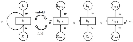
Figure 2. A structure of the recurrent neural network (RNN).

$X_t:$

Input value at time t.

$h_t:$

Hidden state vector at time t.

$h_{t-1}:$

Previous hidden state at time $t-1$.

$\sigma :$

Activation function.

u: 

Weight matrix for input to hidden state.

w: 

Weight matrix for hidden state to next hidden state.

$b_h:$

Bias vector for hidden layer.

v: 

Weight matrix for hidden state to output.

$b_y:$

Output bias term.

$X_{t+1}:$

Predicted value for next time step $t+1$.

For solar forecasting applications, RNNs can process sequences of irradiance and satellite-derived cloud indices to capture how past cloud cover influences current irradiance [51]. Nevertheless, the vanishing gradient problem prevents RNNs from learning reliable dependencies over long periods [52]. It may fail to link early-morning fog with suppressed midday irradiance during extended cloudy periods. Thus, it can be unreliable for day-ahead forecasts.

3.3. Long Short-Term Memory Model

The Long Short-Term Memory (LSTM) model improves solar forecasting by solving RNNs’ vanishing gradient issue through gated memory cells, as demonstrated in Figure 3. The LSTM network can be represented by:

$$\begin{array}{cc}\hfill f_t& =\sigma (W_f·[h_{t-1},x_t]+b_f)\hfill \\ \hfill i_t& =\sigma (W_i·[h_{t-1},x_t]+b_i)\hfill \\ \hfill {\tilde{C}}_t& =tanh(W_C·[h_{t-1},x_t]+b_C)\hfill \\ \hfill C_t& =f_t\odot C_{t-1}+i_t\odot {\tilde{C}}_t\hfill \\ \hfill o_t& =\sigma (W_o·[h_{t-1},x_t]+b_o)\hfill \\ \hfill h_t& =o_t\odot tanh\left(C_t\right)\hfill \\ \hfill X_t& =W_y{h}_t+b_y\hfill \end{array}$$

(12)

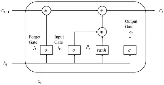
Figure 3. A structure of the long short-term memory network (LSTM).

$x_t:$

Input vector at time t.

${\mathbf{h}}_t:$

Hidden state vector at time t.

${\mathbf{h}}_{t-1}:$

Previous hidden state from time $t-1$.

${\mathbf{C}}_t:$

Cell state vector (long-term memory).

${\mathbf{C}}_{t-1}:$

Previous cell state from time $t-1$.

${\mathbf{f}}_t:$

Forget gate activation vector, values in [0,1].

${\mathbf{i}}_t:$

Input gate activation vector, values in [0,1].

${\mathbf{o}}_t:$

Output gate activation vector, values in [0,1].

${\tilde{\mathbf{C}}}_t:$

Candidate cell state vector.

${\mathbf{W}}_f,{\mathbf{W}}_i,{\mathbf{W}}_C,{\mathbf{W}}_o:$

Weight matrices.

${\mathbf{b}}_f,{\mathbf{b}}_i,{\mathbf{b}}_C,{\mathbf{b}}_o:$

Bias vectors.

${\mathbf{W}}_y:$

Output weight matrix.

$b_y:$

Output bias scalar.

$\sigma (·):$

Sigmoid activation: $\sigma \left(x\right)={\displaystyle \frac{1}{1+e^{-x}}}$, output range [0,1].

$tanh(·):$

Hyperbolic tangent: $tanh\left(x\right)={\displaystyle \frac{e^x-e^{-x}}{e^x+e^{-x}}}$, output range [−1,1].

⊙

Element-wise product operation.

$X_t:$

Predicted irradiance at time t (W/m²).

The LSTM’s gating mechanism mirrors how meteorologists track weather patterns. Consider forecasting solar irradiance during a developing cloud system. The Forget Gate ($f_t$) determines which past weather information becomes irrelevant. For instance, yesterday’s clear-sky conditions may be “forgotten” when a new weather front arrives. The Input Gate ($i_t$) decides which new observations are important. When detecting cumulus cloud formation at 10 am, this gate emphasizes this critical information for afternoon predictions. The Cell State ($C_t$) acts as the model’s “weather memory,” maintaining persistent patterns like multi-day weather systems or seasonal trends that affect long-term irradiance. The Output Gate ($o_t$) filters the relevant information for the current prediction. During stable conditions, it may rely heavily on recent history, while during transitions, it emphasizes new atmospheric changes. Imagine predicting noon irradiance at 9 AM. The LSTM examines morning cloud development (input gate), remembers if a weather system has been building for days (cell state), forgets irrelevant data from last week’s different weather pattern (forget gate), and outputs a prediction considering both current conditions and persistent trends (output gate).

The input, forget, and output gates are utilized to dynamically regulate the information flow, preserving context through sunrise–sunset transitions and multi-day weather patterns [24]. Therefore, LSTM can correlate the thickness of the cloud at dawn with the recovery of the afternoon irradiance, which is impossible for standard RNNs. This capability enables longer-term forecasts with reduced prediction errors [25]. However, LSTM processes only unidirectional sequences from past to future, which can overlook future-influenced patterns such as night cloud build-up that could affect sunset irradiance [53].

3.4. Bidirectional Long Short-Term Memory Model

Bidirectional long short-term memory (BiLSTM) models overcome unidirectional limitations by processing sequences in both forward and backward directions, as illustrated in Figure 4. The BiLSTM model is defined through two passes:

$$\begin{array}{cc}\hfill {\overrightarrow{f}}_t& =\sigma \left(W_f^{\to }[{\overrightarrow{h}}_{t-1},x_t]+b_f^{\to }\right)\hfill \\ \hfill {\overrightarrow{i}}_t& =\sigma \left(W_i^{\to }[{\overrightarrow{h}}_{t-1},x_t]+b_i^{\to }\right)\hfill \\ \hfill {\overrightarrow{\tilde{C}}}_t& =tanh\left(W_C^{\to }[{\overrightarrow{h}}_{t-1},x_t]+b_C^{\to }\right)\hfill \\ \hfill {\overrightarrow{C}}_t& ={\overrightarrow{f}}_t\odot {\overrightarrow{C}}_{t-1}+{\overrightarrow{i}}_t\odot {\overrightarrow{\tilde{C}}}_t\hfill \\ \hfill {\overrightarrow{o}}_t& =\sigma \left(W_o^{\to }[{\overrightarrow{h}}_{t-1},x_t]+b_o^{\to }\right)\hfill \\ \hfill {\overrightarrow{h}}_t& ={\overrightarrow{o}}_t\odot tanh\left({\overrightarrow{C}}_t\right)\hfill \\ \hfill {\overleftarrow{f}}_t& =\sigma \left(W_f^{\leftarrow }[{\overleftarrow{h}}_{t+1},x_t]+b_f^{\leftarrow }\right)\hfill \\ \hfill {\overleftarrow{i}}_t& =\sigma \left(W_i^{\leftarrow }[{\overleftarrow{h}}_{t+1},x_t]+b_i^{\leftarrow }\right)\hfill \\ \hfill {\overleftarrow{\tilde{C}}}_t& =tanh\left(W_C^{\leftarrow }[{\overleftarrow{h}}_{t+1},x_t]+b_C^{\leftarrow }\right)\hfill \\ \hfill {\overleftarrow{C}}_t& ={\overleftarrow{f}}_t\odot {\overleftarrow{C}}_{t+1}+{\overleftarrow{i}}_t\odot {\overleftarrow{\tilde{C}}}_t\hfill \\ \hfill {\overleftarrow{o}}_t& =\sigma \left(W_o^{\leftarrow }[{\overleftarrow{h}}_{t+1},x_t]+b_o^{\leftarrow }\right)\hfill \\ \hfill {\overleftarrow{h}}_t& ={\overleftarrow{o}}_t\odot tanh\left({\overleftarrow{C}}_t\right)\hfill \\ \hfill X_t& =W_y\left[\begin{array}{c}{\overrightarrow{h}}_t\\ {\overleftarrow{h}}_t\end{array}\right]+b_y\hfill \end{array}$$

(13)

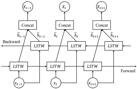
Figure 4. A structure of the bidirectional long short-term memory network (BiLSTM).

$x_t:$

Input at time t;

${\overrightarrow{h}}_t:$

Forward hidden state (past to future context);

${\overleftarrow{h}}_t:$

Backward hidden state (future to past context);

$W^{\to },b^{\to }:$

Forward pass weights/biases;

$W^{\leftarrow },b^{\leftarrow }:$

Backward pass weights/biases;

$W_y,b_y:$

Output layer parameters;

$X_t:$

Prediction at time t.

BiLSTM processes solar data much like analyzing a weather map from two perspectives simultaneously. In the forward direction (${\overrightarrow{h}}_t$), it tracks how morning conditions evolve into afternoon irradiance, following the natural temporal causality of weather development. In the backward direction (${\overleftarrow{h}}_t$), it provides context from future observations back to the present—for example, in training data, knowing that heavy clouds arrived at 3 PM helps better interpret partial cloud cover observed at noon. This is similar to a meteorologist reviewing a day’s weather pattern both chronologically, from morning to evening, and retrospectively, by understanding morning conditions more clearly after seeing how the day unfolded. Such bidirectional analysis captures patterns like “morning fog that clears by noon” more effectively than unidirectional processing.

Two parallel LSTM layers enable the analysis of historical data from opposite directions and merge output to capture dependencies of solar irradiance influenced by impending cloud cover. BiLSTM can reduce forecast errors compared to unidirectional LSTMs [54]. However, it doubles computational cost, making real-time deployment challenging for high-resolution satellite data streams.

3.5. Convolutional Neural Network Model

Convolutional Neural Network (CNN) models represent another major machine learning structure that transforms the extraction of spatial features from sky imagery and satellite data (Figure 5) [26,55]. Using convolutional filters, CNNs can detect cloud textures, edges, and motion vectors from pixel grids, automating tasks that previously relied on manual feature engineering. CNNs can be mathematically defined as follows:

$$\begin{array}{cc}\hfill X_{\mathrm{in}}& ={[X_1,X_2,\dots ,X_w]}^{\top }\hfill \\ \hfill H& =\mathrm{ReLU}\left(W⊛X_{\mathrm{in}}+b\right)\hfill \\ \hfill P& ={\mathrm{MaxPool}}_{s=2}\left(H\right)\hfill \\ \hfill f& =\mathrm{Flatten}\left(H\right)\hfill \\ \hfill X_{t+1}& =W_{\mathrm{out}}f+b_{\mathrm{out}}\hfill \end{array}$$

(14)

Figure 5. A typical structure of the convolutional neural network (CNN).

w: 

Input window size;

k: 

Kernel size;

s: 

Stride/Pool size;

∗:

Convolution operation;

$W^{\left(l\right)}:$

Learnable kernel weights;

$b^{\left(l\right)}:$

Bias term in layer l;

$\mathrm{ReLU}:$

Activation function ReLU;

$\mathrm{MaxPool}:$

Maximum value pooling operation;

$X_{t+1}:$

Predicted value for the next time step.

A CNN processes satellite or sky images by detecting hierarchical spatial patterns. Its convolutional filters act as cloud pattern detectors, where early filters may identify simple features such as edges or cloud boundaries, while deeper filters capture more complex structures like cumulonimbus formations or fog banks. Through this spatial hierarchy, the first layer detects basic features such as cloud edges and brightness gradients, the second layer combines these edges into recognizable cloud shapes like cumulus or stratus, and the third layer identifies larger weather patterns such as frontal systems or convective cells. Pooling operations then provide spatial invariance, ensuring that a cloud’s impact on irradiance is recognized regardless of whether it appears slightly east or west in the image. When processing a sky image, a CNN might first detect dark pixels as clouds, then recognize circular patterns as signs of cumulus formation, and finally track movement across sequential images to predict cloud trajectories, ultimately forecasting that solar panels will be shaded within 30 min.

For irradiance forecasting, a CNN processes geostationary satellite images to predict regional cloud coverage hours ahead. Although a CNN performs well at spatial pattern recognition, it typically ignores temporal evolution. Thus, a standalone CNN may identify cumulus clouds but does not predict their drift direction or dissipation rate [56].

3.6. Graph Neural Network Model

Graph neural network (GNN) models are proposed to address distributed spatial modeling by representing weather stations or PV plants as nodes within a graph. Edges encode geographical distances or atmospheric correlations (e.g., wind-driven cloud propagation between sites). The GNN is expressed as follows:

$$\begin{array}{cc}\hfill \mathcal{G}& =(\mathcal{V},\mathcal{E},X)\hfill \\ \hfill h_i^{(l+1)}& =\sigma \left(W^{\left(l\right)}·{\displaystyle \frac{1}{\left|\mathcal{N}\right(i\left)\right|}}\sum _{j\in \mathcal{N}\left(i\right)}{h}_j^{\left(l\right)}+b^{\left(l\right)}\right)\hfill \\ \hfill {\alpha }_{ij}& ={\displaystyle \frac{exp\left(\mathrm{LeakyReLU}\left(a^{\top }[W{h}_i\parallel W{h}_j]\right)\right)}{{\sum }_{k\in \mathcal{N}\left(i\right)}exp\left(\mathrm{LeakyReLU}\left(a^{\top }[W{h}_i\parallel W{h}_k]\right)\right)}}\hfill \\ \hfill H^{\left(t\right)}& =\mathrm{GraphConvolution}(X^{\left(t\right)},\mathcal{G})\hfill \end{array}$$

(15)

$\mathcal{G}:$

Graph structure representing the solar sensor network.

$\mathcal{V}:$

Set of nodes (vertices), $\left|\mathcal{V}\right|=N$ nodes (sensor locations).

$\mathcal{E}:$

Set of edges, $\left|\mathcal{E}\right|=E$ edges (spatial connections).

$\mathbf{X}:$

Node feature matrix.

${\mathbf{h}}_i^{\left(l\right)}:$

Hidden representation of node i at layer l.

${\mathbf{h}}_i^{(l+1)}:$

Updated representation of node i at layer $l+1$.

$\mathcal{N}\left(i\right):$

Set of neighbor nodes connected to node i.

$\left|\mathcal{N}\right(i\left)\right|:$

Number of neighbors for node i (node degree).

${\mathbf{W}}^{\left(l\right)}:$

Weight matrix at layer l.

${\mathbf{b}}^{\left(l\right)}:$

Bias vector at layer l.

${\alpha }_{ij}:$

Attention weight from node j to node i, ${\sum }_{j\in \mathcal{N}\left(i\right)}{\alpha }_{ij}=1$.

$\mathbf{a}:$

Attention parameter vector (learnable).

‖: 

Concatenation operation for attention computation.

$\mathrm{LeakyReLU}:$

Leaky rectified linear unit with negative slope 0.2.

${\mathbf{H}}^{\left(t\right)}:$

Graph-level output at time t for all nodes.

$\sigma (·):$

Activation function (typically ReLU or sigmoid).

A GNN models a solar sensor network as an interconnected system in which each node, representing a solar measurement station or PV plant, is influenced by its neighbors. The edges encode relationships such as geographical distance, prevailing wind direction, or topographical connections, while message passing simulates how weather patterns, like cloud shadows, propagate across the network. Imagine three solar stations A, B, and C aligned east to west under prevailing westerly winds. If Station A detects a sudden irradiance drop due to cloud cover at 10:00 AM, the GNN propagates this information through the network, weighting the connections by wind speed and direction. The model then predicts that Station B will experience a similar drop at 10:15 AM and Station C at 10:30 AM. Each station’s forecast combines both its own local measurements and the information shared from its neighbors. This process mirrors how regional weather systems impact distributed solar installations, where upstream conditions provide an early warning for downstream sites.

By propagating information through the graph structure, GNNs can forecast irradiance across regions with sparse sensors, which is critical for utility-scale solar farms [57]. Since a GNN reduces regional forecast errors compared to traditional models, it requires precise graph construction. For example, users need to define the connectivity of nodes through atmospheric models, which adds additional complexity.

3.7. Transformer

Transformer architecture bypasses sequential processing utilized by RNNs/LSTMs through self-attention mechanisms.

The transformer, as shown in Figure 6, can be represented as:

$$\begin{array}{cc}\hfill X_{\mathrm{in}}& ={[x_1,x_2,\dots ,x_T]}^{\top }\hfill \\ \hfill \mathrm{PE}(t,2i)& =sin(t/{10000}^{2i/d_{\mathrm{model}}})\hfill \\ \hfill \mathrm{PE}(t,2i+1)& =cos(t/{10000}^{2i/d_{\mathrm{model}}})\hfill \\ \hfill Q^{\left(l\right)}& =X^{(l-1)}{W}_Q^l,K^{\left(l\right)}=X^{(l-1)}{W}_K^l,V^{\left(l\right)}=X^{(l-1)}{W}_V^l\hfill \\ \hfill {\mathrm{Attention}}^{\left(l\right)}& =\mathrm{softmax}\left({\displaystyle \frac{Q^{\left(l\right)}{\left(K^{\left(l\right)}\right)}^{\top }}{\sqrt{d_k}}}\right)V^{\left(l\right)}\hfill \\ \hfill X^{\prime \left(l\right)}& =\mathrm{LayerNorm}\left(X^{(l-1)}+{\mathrm{MultiHead}}^{\left(l\right)}(Q,K,V)\right)\hfill \\ \hfill X^{\left(l\right)}& =\mathrm{LayerNorm}\left(X^{\prime \left(l\right)}+{\mathrm{FFN}}^{\left(l\right)}\left(X^{\prime \left(l\right)}\right)\right)\hfill \\ \hfill Y^{\prime \left(l\right)}& =\mathrm{LayerNorm}\left(Y^{(l-1)}+{\mathrm{MaskedMultiHead}}^{\left(l\right)}\left(Y^{(l-1)}\right)\right)\hfill \\ \hfill Y^{\prime \prime \left(l\right)}& =\mathrm{LayerNorm}\left(Y^{\prime \left(l\right)}+{\mathrm{MultiHead}}^{\left(l\right)}(Y^{\prime \left(l\right)},X^{\left(N\right)},X^{\left(N\right)})\right)\hfill \\ \hfill Y^{\left(l\right)}& =\mathrm{LayerNorm}\left(Y^{\prime \prime \left(l\right)}+{\mathrm{FFN}}^{\left(l\right)}\left(Y^{\prime \prime \left(l\right)}\right)\right)\hfill \\ \hfill \widehat{Y}& =Y^{\left(N\right)}{W}_{\mathrm{out}}+b_{\mathrm{out}}\hfill \end{array}$$

(16)

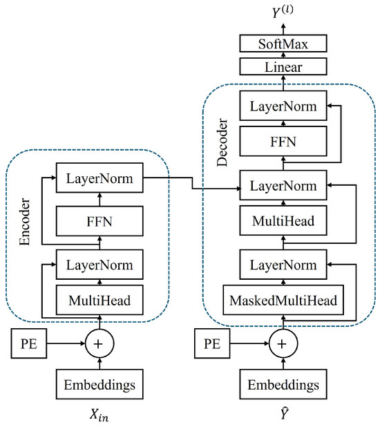
Figure 6. A typical architecture of the transformer network.

${\mathbf{X}}_{in}:$

Input sequence matrix.

T: 

Sequence length (number of time steps).

$d_{model}:$

Model dimension (hidden state size).

$\mathrm{PE}(t,i):$

Positional encoding for position t.

${\mathbf{Q}}^{\left(l\right)},{\mathbf{K}}^{\left(l\right)},{\mathbf{V}}^{\left(l\right)}:$

Query, Key, Value matrices at layer l.

$d_k=d_v:$

Dimension of keys and values, $d_k=d_{model}/h$.

h: 

Number of attention heads for multi-head attention.

${\mathbf{W}}_Q^l,{\mathbf{W}}_K^l,{\mathbf{W}}_V^l:$

Projection matrices.

${\mathrm{Attention}}^{\left(l\right)}:$

Attention output matrix.

$\sqrt{d_k}:$

Scaling factor to prevent gradient saturation.

$\mathrm{softmax}(·):$

Row-wise softmax normalization.

${\mathrm{MultiHead}}^{\left(l\right)}:$

Concatenation of h attention heads.

$\mathrm{LayerNorm}:$

Layer normalization with learnable parameters.

${\mathrm{FFN}}^{\left(l\right)}:$

Feedforward network: $max(0,\mathbf{x}{\mathbf{W}}_1+{\mathbf{b}}_1){\mathbf{W}}_2+{\mathbf{b}}_2$.

${\mathbf{W}}_1:$

First FFN weight matrix.

${\mathbf{W}}_2:$

Second FFN weight matrix.

$d_{ff}:$

Feedforward dimension (typically $4\times d_{model}$).

N: 

Number of encoder/decoder layers.

$\mathrm{Mask}:$

Causal mask matrix preventing attention to future positions.

${\mathbf{W}}_{out},{\mathbf{b}}_{out}:$

Final output projection parameters.

$\widehat{\mathbf{Y}}:$

Output predictions.

The Transformer’s self-attention mechanism determines which historical time points are most relevant for making the current prediction. High attention to similar times on the previous day reflects recognition of diurnal patterns, while strong attention to recent hours captures the influence of evolving weather systems. Likewise, attention to the same time last week may reveal weekly trends, such as industrial load cycles affecting local meteorology. Importantly, attention weights vary depending on weather stability, adapting the model’s focus as conditions change.

By weighing all time steps in sequence simultaneously, it captures long-range dependencies. Therefore, it can even link aerosol levels in the morning with the attenuation of afternoon irradiance. Moreover, positional embeddings of the transformer structure preserve temporal order without recurrence, enabling parallelized training on years of global irradiance data.

Transformer can outperform most prediction models by achieving lower forecasting errors [58]. The most significant barrier lies in its computational complexity, which limits its application for edge deployment scenarios.

3.8. Hybrid Network

Hybrid neural networks combine complementary machine learning components to overcome inherent limitations of single-model approaches. Unlike standalone CNNs, RNNs, or Transformers, hybrid architectures integrate specialized submodules that concurrently handle spatial, temporal, and relational dependencies—mirroring the multiscale physics of solar irradiance variability.

CNN-LSTM serves as an example to demonstrate hybrid neural networks. Convolutional layers process raw satellite imagery to extract localized cloud textures and motion vectors, while LSTM submodules interpret these features as temporal sequences for modeling cloud advection dynamics across forecast horizons. This spatio-temporal coupling enables more precise forecasting of irradiance ramps during convective cloud events compared to isolated models [59]. Similarly, GNN-LSTM architectures construct dynamic graphs of regional sensor networks, where graph layers propagate cloud shadow movements across PV nodes, and LSTMs forecast site-specific irradiance for utility-scale PV systems in large regions (as depicted in Figure 7).

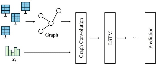
Figure 7. A typical structure of the graph neural network (GNN) plus LSTM for spatio-temporal forecasting.

Transformers further enhance hybrid designs by enabling global context awareness. In CNN–Transformer architectures, convolutional encoders extract high-resolution sky images into compact feature tokens, while transformer decoders apply self-attention to correlate long-range atmospheric states. This approach resolves computational bottlenecks of pure vision transformers while capturing cross-hour dependencies.

Hybrid neural networks represent the inevitable future of solar irradiance forecasting, as they synergistically address the multiscale, multimodal nature of atmospheric dynamics that single-model architectures fundamentally cannot handle.

4. Comparative Discussions

This section presents a systematic comparison of nineteen time-series forecasting models for TSSIF, which encompasses traditional statistical methods and machine learning approaches. Table 1 summarizes these models across seven evaluation criteria: computational complexity, accuracy, data requirements, robustness, application scenarios, and key advantages and drawbacks. The following sections analyze each criterion in detail, examining how model characteristics can affect their performance in solar irradiance forecasting applications. This comparative framework facilitates model selection based on specific operational requirements, including computational resources, data availability, and prediction horizons.

Table 1. Comprehensive comparison of time-series forecasting models applied to solar forecasting.

Model	Complexity	Accuracy	Data Req.	Robustness	Application	Key Advantage	Key Drawback
Traditional Statistical Models
AR	$O(n·p)$	Low	Small	Low	Short	Simple, interpretable	Linear assumptions; fails during sudden cloud cover or storms
MA	$O(n·q)$	Low	Small	Low	Short	Handles shocks well	Only captures short memory; poor in multi-day weather systems
ARMA	$O(n·(p+q\left)\right)$	Low–Mid	Small	Low–Mid	Short	Combines AR and MA benefits	Requires stationarity; fails during seasonal transitions and extreme events
ARIMA	$O(n·(p+d+q\left)\right)$	Mid	Small–Mid	Mid	Short–Mid	Handles non-stationary data	Parameter selection difficulty; poor performance in fog/dust events
ARCH	$O(n·p)$	Mid	Mid	Low–Mid	Short	Models volatility clustering	Assumes symmetric volatility; fails in asymmetric storm patterns
GARCH	$O(n·(p+q\left)\right)$	Mid	Mid	Mid	Short–Mid	Captures volatility persistence	Complex parameters; struggles with sudden atmospheric pressure drops
VAR	$O(n·k^2·p)$	Mid	Mid	Mid	Short–Mid	Multivariate relationships	Curse of dimensionality; unstable during rare weather combinations
TVAR	$O(n^2·k^2)$	Mid–High	Mid–Big	Mid	Short–Mid	Regime-switching capability	Threshold selection; regime detection fails in unprecedented events
Machine Learning Models
Lasso	$O(n·p^2)$	Mid	Mid	Mid–High	Short–Mid	Feature selection built in	Linear relationships only; cannot capture extreme nonlinearities
FNN	$O(n·m·l)$	Mid	Mid–Big	Mid	Short–Mid	Universal approximator	No temporal memory; fails in rapid weather transitions
RNN	$O(n·T·h^2)$	Mid–High	Big	Low–Mid	Mid	Sequential processing	Vanishing gradient; poor in extended unusual weather periods
LSTM	$O(n·T·h^2)$	High	Big	High	Mid–Long	Long-term dependencies	High computational cost; degrades with out-of-distribution extremes
BiLSTM	$O(n·T·h^2·2)$	High	Big	High	Mid–Long	Bidirectional context	Even higher complexity; requires future data unavailable in real time
CNN	$O(n·T·k·c^2)$	Mid–High	Mid–Big	Mid–High	Short–Mid	Parallel processing, fast	Limited sequential modeling; misses temporal storm development
GNN	$O(n·E·d^2)$	High	Big	Mid–High	Mid–Long	Graph structure exploitation	Requires graph construction; topology fails in extreme spatial events
Transformer	$O(n·T^2·d)$	High	Big	High	Long	Attention mechanism	Very high memory; attention dilution in chaotic weather
CNN + RNN	$O(n·T·(k·c^2+h^2))$	High	Big	High	Mid–Long	Feature extraction + sequential	Complex architecture; component failures cascade in extremes
GNN + LSTM	$O(n·(E·d^2+T·h^2))$	High	Big	High	Long	Spatial–temporal modeling	Very complex; spatial assumptions break in hurricane conditions

n: Number of training samples; p: Order of autoregressive (AR) terms; q: Order of moving-average (MA) terms; d: Degree of differencing (ARIMA); k: Number of variables (VAR) or kernel size (CNN); T: Sequence/time series length; h: Number of hidden units in neural networks; m: Number of input features; l: Number of layers in neural networks; c: Number of channels in convolutional networks; E: Number of edges in graph structure; d: Embedding/feature dimension (Transformer, GNN).

Computational complexity is a critical factor for solar irradiance forecasting due to the need for real-time predictions in grid integration and energy management systems. Traditional statistical models (AR, MA, ARMA, ARIMA) with complexity $O(n·p)$ to $O(n·(p+d+q\left)\right)$ offer the fastest computation times, making them suitable for embedded systems in solar farms or real-time grid balancing applications where millisecond-level response times are required. The volatility models (ARCH, GARCH) maintain relatively low complexity $O(n·(p+q\left)\right)$ while capturing the heteroscedastic nature of solar irradiance, which is particularly useful for modeling cloud-induced variability. Machine learning approaches like Lasso with $O(n·p^2)$ provide a middle ground, offering reasonable computation times while handling multiple meteorological features. Deep learning models present a significant computational burden, with RNNs and LSTMs requiring $O(n·pT·h^2)$ operations, making them suitable primarily for day-ahead forecasting where computation time is less critical. The Transformer’s $O(n·T^2·d)$ complexity becomes particularly challenging for high-frequency solar data (minute-level recordings), often requiring down-sampling or windowing strategies. Hybrid models such as CNN + RNN and GNN + LSTM, while offering superior performance, demand the highest computational resources, typically necessitating a dedicated GPU infrastructure for operational deployment.

Accuracy in solar irradiance forecasting directly impacts grid stability control, making it perhaps the most crucial performance metric. Traditional models (AR, MA, ARMA) demonstrate low accuracy for solar irradiance due to their inability to capture complex nonlinear relationships between meteorological variables and solar radiation. ARIMA shows moderate improvement by handling the non-stationary nature of solar data across seasons for short-term forecasts. The ARCH and GARCH models provide medium accuracy with a particular strength in quantifying prediction uncertainty during volatile weather conditions, which is essential for risk management in solar energy trading. Deep learning models significantly outperform traditional approaches for hourly forecasts by learning complex temporal dependencies between cloud cover patterns, atmospheric conditions, and irradiance levels. CNNs excel when combined with satellite imagery data, extracting spatial features from cloud formations to improve very short-term forecasts. Transformer models demonstrate exceptional accuracy for day-ahead predictions by capturing long-range dependencies between weather patterns, though their performance advantage diminishes for now-casting applications. Hybrid models consistently achieve the highest accuracy by combining spatial weather patterns from CNNs or GNNs with temporal dynamics from LSTMs, particularly when integrating multiple data sources, including numerical weather predictions, satellite imagery, and ground-based measurements.

A quantitative performance evaluation across public datasets provides concrete evidence of model capabilities, as summarized in Table 2 sourced from [57]. These tests are performed based on the data sourced from the U.S. National Renewable Energy Laboratory. The system includes 17 silicon radiometers dispersively distributed at the Kalaeloa Airport on Oahu Island, Hawaii. Each location deploys a solar sensor to collect the time-series solar data. These quantitative results confirm that while traditional models remain acceptable for prediction results, machine learning and hybrid approaches offer superior accuracy when resources permit, particularly for operational solar forecasting applications requiring high precision.

Table 2. Quantitative comparison of prediction accuracy.

Model		Evaluation Metrics
		MAE	MAPE	RMSE
Statistical Methods	ARIMA	0.27	26.69	0.35
	LR	0.08	18.11	0.095
	MA	0.076	17.21	0.089
	SVM	0.082	18.44	0.097
Machine Learning Approaches	GRU	0.027	6.37	0.027
	RNN	0.022	5.35	0.023
	LSTM	0.024	5.13	0.031
	Attentional Network	0.019	4.51	0.022
	CNN + LSTM	0.014	3.61	0.017
	GNN + LSTM	0.012	2.86	0.013

MAE: Mean Absolute Error; MAPE: Mean Absolute Percentage Error; RMSE: Root Mean Square Error.

The data requirements for solar irradiance forecasting models significantly impact their practical deployment, since the availability of historical solar data varies greatly between geographic regions and installation ages. Traditional statistical models (AR, MA, ARMA, ARIMA) require minimal data (typically 3–6 months of hourly recordings), making them ideal for newly commissioned solar installations or regions with limited historical records, though this comes at a cost of reduced accuracy and an inability to capture annual seasonal patterns. The ARCH and GARCH models need moderate amounts of data (1–2 years) to properly estimate volatility parameters, particularly important for capturing the full range of weather-induced variability across seasons. Machine learning approaches like Lasso require medium-sized datasets (2–3 years) to achieve stable feature selection, particularly when incorporating multiple meteorological variables such as temperature, humidity, wind speed, and atmospheric pressure. Deep learning models present the most stringent data requirements, with RNNs and LSTMs typically needing 3–5 years of hourly or sub-hourly data to avoid overfitting, while also requiring diverse weather conditions in the training set to generalize well to extreme events like storms or unusual cloud patterns. Transformers demand even larger datasets (5+ years) to fully leverage their attention mechanisms, often necessitating data augmentation techniques or transfer learning from regions with richer historical records. GNNs require not just temporal data but also spatial network information from multiple measurement stations, making them suitable primarily for regional or national-scale forecasting where extensive sensor networks exist. The data quality requirements also escalate with model complexity, as deep learning models are more sensitive to missing values, sensor drift, and measurement errors, necessitating sophisticated preprocessing pipelines.

Robustness in solar irradiance forecasting encompasses the model’s ability to maintain performance under diverse weather conditions, seasonal variations, equipment degradation, and data quality issues that are inherent to solar monitoring systems. Traditional models (AR, MA, ARMA) exhibit low robustness, particularly failing during rapid weather transitions such as passing cloud fronts or sudden storms, with prediction errors often doubling during these events compared to clear-sky conditions. ARIMA shows improved robustness through its differencing mechanism, which helps adapt to seasonal shifts and long-term trends caused by atmospheric changes or solar panel degradation, though it still struggles with sudden nonlinear events. The ARCH and GARCH models demonstrate medium robustness with a particular strength in maintaining calibrated uncertainty estimates during volatile periods, crucial for conservative grid management strategies during unstable weather. Lasso regression offers medium-high robustness through its inherent regularization, preventing overfitting to specific weather patterns and maintaining stable performance across seasons, though it cannot adapt to fundamentally new weather regimes. Deep learning models show varied robustness characteristics: standard RNNs suffer from low to medium robustness due to gradient instability and a tendency to overfit to recent patterns, while LSTMs and BiLSTMs achieve high robustness through their gating mechanisms that filter out noise and maintain long-term memory of seasonal patterns. CNNs demonstrate medium–high robustness when properly regularized with dropout and data augmentation, particularly effective at handling partial shading and localized cloud effects. Transformers exhibit high robustness by learning multiple attention patterns for different weather scenarios, effectively switching between forecasting strategies based on atmospheric conditions. Hybrid models achieve the highest robustness by combining complementary strengths, such as CNN’s spatial pattern recognition for cloud detection with LSTM’s temporal stability, maintaining acceptable performance even during rare meteorological events.

The choice of forecasting model for solar irradiance critically depends on the specific application time frame, as different operational decisions require predictions at vastly different horizons with varying accuracy–speed trade-offs. For very short-term forecasting (0–30 min ahead), essential for real-time grid frequency regulation and ramp-rate control, traditional models (AR, MA, ARMA) and CNNs processing sky imagery provide an optimal balance of speed and sufficient accuracy, with sub-minute computation times enabling rapid response to cloud movements. Short-term forecasting (30 min to 6 h), crucial for intraday energy trading and battery storage dispatch, benefits most from the ARIMA, GARCH, and standard LSTM models that can capture diurnal patterns while remaining computationally tractable for operational deployment. Medium-term predictions (6–48 h), vital for day-ahead market bidding and conventional generator scheduling, achieve best results with advanced deep learning approaches—particularly BiLSTMs and Transformers that can integrate numerical weather predictions with historical patterns to anticipate weather system movements. Long-term forecasting (2–7 days), necessary for maintenance scheduling and weekly energy planning, relies almost exclusively on Transformer architectures and hybrid GNN + LSTM models that can process large-scale atmospheric data and capture complex teleconnections between distant weather systems. The application context also influences model selection beyond just the time horizon: grid-connected utility-scale solar farms can afford complex Transformer models with a dedicated computational infrastructure, while distributed rooftop solar systems require lightweight ARIMA or simple LSTM models that can run on edge devices. Furthermore, critical applications like hospital microgrids may prefer ensemble approaches combining multiple models to ensure reliability, while commercial installations might opt for single models that minimize computational costs while meeting basic accuracy requirements.

5. Conclusions

This paper presents a comprehensive review and comparative analysis of nineteen data-driven approaches for time-series solar irradiance forecasting, spanning from traditional statistical methods to state-of-the-art deep learning architectures. Our systematic evaluation reveals clear trade-offs between computational complexity, accuracy, data requirements, and robustness across different model categories. Traditional statistical models (AR, MA, ARMA, ARIMA) remain valuable for real-time applications with limited computational resources, achieving sufficient accuracy for very short-term predictions despite their linear assumptions. Deep learning approaches, particularly LSTMs and Transformers, demonstrate superior accuracy for medium- to long-term forecasting by capturing complex nonlinear patterns and long-range dependencies, though at the cost of increased computational demands and extensive data requirements. Hybrid architectures such as CNN + LSTM and GNN + LSTM emerge as the most promising solutions, successfully balancing accuracy with practical constraints by combining the complementary strengths of different model types.

The comparative framework presented provides actionable guidance for model selection based on specific operational requirements. For grid operators requiring sub-minute response times, lightweight traditional models or simple CNNs offer optimal solutions. Energy traders and utility-scale operations can benefit from LSTM-based models for day-ahead forecasting, while Transformer architectures excel at long-term predictions when computational resources permit. Critical challenges remain, including handling extreme weather events, reducing computational complexity for edge deployment, and addressing data scarcity in new installations. Future research should focus on transfer learning for data-limited scenarios, physics-informed neural networks for improved interpretability, and adaptive ensemble methods that dynamically select models based on weather conditions. As solar energy continues its rapid expansion, the insights from this comprehensive review will guide researchers and practitioners in selecting and implementing the appropriate forecasting solution, ultimately supporting the integration of solar power into sustainable energy systems.

While this review provides comprehensive technical analysis of forecasting models, future work can systematically evaluate these practical deployment factors through comprehensive techno-economic analysis, including detailed cost–benefit studies comparing the total cost of ownership across different model architectures for various deployment scales, real-time performance benchmarking under operational constraints including communication latency and computational resource limitations, reliability and maintenance requirement assessment through long-term field deployments, development of deployment-aware model selection frameworks that balance technical performance with engineering constraints, and investigation of edge computing solutions and model compression techniques to enable advanced algorithms on resource-constrained hardware.

References

- Yang, D.; Dong, Z. Operational photovoltaics power forecasting using seasonal time series ensemble. Sol. Energy 2018, 166, 529–541. [Google Scholar] [CrossRef]
- Xiao, W. Photovoltaic Power System: Modeling, Design and Control, 1st ed.; Wiley: Hoboken, NJ, USA, 2017. [Google Scholar]
- Wang, H.; Liu, Y.; Zhou, B.; Li, C.; Cao, G.; Voropai, N.; Barakhtenko, E. Taxonomy research of artificial intelligence for deterministic solar power forecasting. Energy Convers. Manag. 2020, 214, 112909. [Google Scholar] [CrossRef]
- Impram, S.; Varbak Nese, S.; Oral, B. Challenges of renewable energy penetration on power system flexibility: A survey. Energy Strategy Rev. 2020, 31, 100539. [Google Scholar] [CrossRef]
- Ahmed, S.D.; Al-Ismail, F.S.M.; Shafiullah, M.; Al-Sulaiman, F.A.; El-Amin, I.M. Grid Integration Challenges of Wind Energy: A Review. IEEE Access 2020, 8, 10857–10878. [Google Scholar] [CrossRef]
- Lei, X.; Zhong, J.; Chen, Y.; Shao, Z.; Jian, L. Grid integration of electric vehicles within electricity and carbon markets: A comprehensive overview. eTransportation 2025, 25, 100435. [Google Scholar] [CrossRef]
- Sampath Kumar, D.; Gandhi, O.; Rodríguez-Gallegos, C.D.; Srinivasan, D. Review of power system impacts at high PV penetration Part II: Potential solutions and the way forward. Sol. Energy 2020, 210, 202–221. [Google Scholar] [CrossRef]
- Ahmad, S.; Shafiullah, M.; Ahmed, C.B.; Alowaifeer, M. A Review of Microgrid Energy Management and Control Strategies. IEEE Access 2023, 11, 21729–21757. [Google Scholar] [CrossRef]
- Jiao, X.; Yang, T.; Li, X.; Ding, S.; Xiao, W. A DC Side Power Ramp Rate Control Strategy for High Performance and Low Cost PV Systems. CPSS Trans. Power Electron. Appl. 2023, 8, 128–136. [Google Scholar] [CrossRef]
- Sukumar, S.; Marsadek, M.; Agileswari, K.; Mokhlis, H. Ramp-rate control smoothing methods to control output power fluctuations from solar photovoltaic (PV) sources—A review. J. Energy Storage 2018, 20, 218–229. [Google Scholar] [CrossRef]
- Akram, U.; Nadarajah, M.; Shah, R.; Milano, F. A review on rapid responsive energy storage technologies for frequency regulation in modern power systems. Renew. Sustain. Energy Rev. 2020, 120, 109626. [Google Scholar] [CrossRef]
- Kebede, A.A.; Kalogiannis, T.; Van Mierlo, J.; Berecibar, M. A comprehensive review of stationary energy storage devices for large scale renewable energy sources grid integration. Renew. Sustain. Energy Rev. 2022, 159, 112213. [Google Scholar] [CrossRef]
- Das, U.K.; Tey, K.S.; Seyedmahmoudian, M.; Mekhilef, S.; Idris, M.Y.I.; Van Deventer, W.; Horan, B.; Stojcevski, A. Forecasting of photovoltaic power generation and model optimization: A review. Renew. Sustain. Energy Rev. 2018, 81, 912–928. [Google Scholar] [CrossRef]
- Sweeney, C.; Bessa, R.J.; Browell, J.; Pinson, P. The future of forecasting for renewable energy. WIREs Energy Environ. 2020, 9, e365. [Google Scholar] [CrossRef]
- Diagne, M.; David, M.; Lauret, P.; Boland, J.; Schmutz, N. Review of solar irradiance forecasting methods and a proposition for small-scale insular grids. Renew. Sustain. Energy Rev. 2013, 27, 65–76. [Google Scholar] [CrossRef]
- Antonanzas, J.; Osorio, N.; Escobar, R.; Urraca, R.; de Pison, F.M.; Antonanzas-Torres, F. Review of photovoltaic power forecasting. Sol. Energy 2016, 136, 78–111. [Google Scholar] [CrossRef]
- Lauret, P.; David, M.; Pedro, H.T.C. Probabilistic Solar Forecasting Using Quantile Regression Models. Energies 2017, 10, 1591. [Google Scholar] [CrossRef]
- Huang, Q.; Wei, S. Improved quantile convolutional neural network with two-stage training for daily-ahead probabilistic forecasting of photovoltaic power. Energy Convers. Manag. 2020, 220, 113085. [Google Scholar] [CrossRef]
- Voyant, C.; Notton, G.; Kalogirou, S.; Nivet, M.L.; Paoli, C.; Motte, F.; Fouilloy, A. Machine learning methods for solar radiation forecasting: A review. Renew. Energy 2017, 105, 569–582. [Google Scholar] [CrossRef]
- Box, G.E.P.; Jenkins, G. Time Series Analysis, Forecasting and Control; Holden-Day, Inc.: San Francisco, CA, USA, 1990. [Google Scholar]
- Reikard, G. Predicting solar radiation at high resolutions: A comparison of time series forecasts. Sol. Energy 2009, 83, 342–349. [Google Scholar] [CrossRef]
- Pedro, H.T.; Coimbra, C.F. Assessment of forecasting techniques for solar power production with no exogenous inputs. Sol. Energy 2012, 86, 2017–2028. [Google Scholar] [CrossRef]
- Ahmed, R.; Sreeram, V.; Mishra, Y.; Arif, M. A review and evaluation of the state-of-the-art in PV solar power forecasting: Techniques and optimization. Renew. Sustain. Energy Rev. 2020, 124, 109792. [Google Scholar] [CrossRef]
- Qing, X.; Niu, Y. Hourly day-ahead solar irradiance prediction using weather forecasts by LSTM. Energy 2018, 148, 461–468. [Google Scholar] [CrossRef]
- Wang, K.; Qi, X.; Liu, H. Photovoltaic power forecasting based LSTM-Convolutional Network. Energy 2019, 189, 116225. [Google Scholar] [CrossRef]
- Si, Z.; Yang, M.; Yu, Y.; Ding, T. Photovoltaic power forecast based on satellite images considering effects of solar position. Appl. Energy 2021, 302, 117514. [Google Scholar] [CrossRef]
- Khodayar, M.; Wang, J. Spatio-Temporal Graph Deep Neural Network for Short-Term Wind Speed Forecasting. IEEE Trans. Sustain. Energy 2019, 10, 670–681. [Google Scholar] [CrossRef]
- Lin, Y.; Koprinska, I.; Rana, M.; Troncoso, A. Solar Power Forecasting Based on Pattern Sequence Similarity and Meta-learning. In Artificial Neural Networks and Machine Learning—ICANN 2020 29th International Conference on Artificial Neural Networks, Bratislava, Slovakia, 15–18 September 2020; Farkaš, I., Masulli, P., Wermter, S., Eds.; Springer: Cham, Switzerland, 2020; pp. 271–283. [Google Scholar]
- Kim, J.; Obregon, J.; Park, H.; Jung, J.Y. Multi-step photovoltaic power forecasting using transformer and recurrent neural networks. Renew. Sustain. Energy Rev. 2024, 200, 114479. [Google Scholar] [CrossRef]
- Liu, Q.; Shen, Y.; Wu, L.; Li, J.; Zhuang, L.; Wang, S. A hybrid FCW-EMD and KF-BA-SVM based model for short-term load forecasting. CSEE J. Power Energy Syst. 2018, 4, 226–237. [Google Scholar] [CrossRef]
- Rajagukguk, R.A.; Ramadhan, R.A.; Lee, H.J. A Review on Deep Learning Models for Forecasting Time Series Data of Solar Irradiance and Photovoltaic Power. Energies 2020, 13, 6623. [Google Scholar] [CrossRef]
- Yang, D.; Alessandrini, S.; Antonanzas, J.; Antonanzas-Torres, F.; Badescu, V.; Beyer, H.G.; Blaga, R.; Boland, J.; Bright, J.M.; Coimbra, C.F.; et al. Verification of deterministic solar forecasts. Sol. Energy 2020, 210, 20–37. [Google Scholar] [CrossRef]
- Notton, G.; Nivet, M.L.; Voyant, C.; Paoli, C.; Darras, C.; Motte, F.; Fouilloy, A. Intermittent and stochastic character of renewable energy sources: Consequences, cost of intermittence and benefit of forecasting. Renew. Sustain. Energy Rev. 2018, 87, 96–105. [Google Scholar] [CrossRef]
- Li, B.; Zhang, J. A review on the integration of probabilistic solar forecasting in power systems. Sol. Energy 2020, 210, 68–86. [Google Scholar] [CrossRef]
- Mayer, M.J.; Gróf, G. Extensive comparison of physical models for photovoltaic power forecasting. Appl. Energy 2021, 283, 116239. [Google Scholar] [CrossRef]
- Brinkworth, B. Autocorrelation and stochastic modelling of insolation sequences. Sol. Energy 1977, 19, 343–347. [Google Scholar] [CrossRef]
- Dong, J.; Olama, M.M.; Kuruganti, T.; Melin, A.M.; Djouadi, S.M.; Zhang, Y.; Xue, Y. Novel stochastic methods to predict short-term solar radiation and photovoltaic power. Renew. Energy 2020, 145, 333–346. [Google Scholar] [CrossRef]
- Yang, D.; Kleissl, J.; Gueymard, C.A.; Pedro, H.T.; Coimbra, C.F. History and trends in solar irradiance and PV power forecasting: A preliminary assessment and review using text mining. Sol. Energy 2018, 168, 60–101. [Google Scholar] [CrossRef]
- Inman, R.H.; Pedro, H.T.; Coimbra, C.F. Solar forecasting methods for renewable energy integration. Prog. Energy Combust. Sci. 2013, 39, 535–576. [Google Scholar] [CrossRef]
- David, M.; Ramahatana, F.; Trombe, P.; Lauret, P. Probabilistic forecasting of the solar irradiance with recursive ARMA and GARCH models. Sol. Energy 2016, 133, 55–72. [Google Scholar] [CrossRef]
- Jiang, P.; Ma, X. A hybrid forecasting approach applied in the electrical power system based on data preprocessing, optimization and artificial intelligence algorithms. Appl. Math. Model. 2016, 40, 10631–10649. [Google Scholar] [CrossRef]
- Lauret, P.; David, M.; Pinson, P. Verification of solar irradiance probabilistic forecasts. Sol. Energy 2019, 194, 254–271. [Google Scholar] [CrossRef]
- Alsharif, M.H.; Younes, M.K.; Kim, J. Time Series ARIMA Model for Prediction of Daily and Monthly Average Global Solar Radiation: The Case Study of Seoul, South Korea. Symmetry 2019, 11, 240. [Google Scholar] [CrossRef]
- Liu, G.; Qin, H.; Shen, Q.; Lyv, H.; Qu, Y.; Fu, J.; Liu, Y.; Zhou, J. Probabilistic spatiotemporal solar irradiation forecasting using deep ensembles convolutional shared weight long short-term memory network. Appl. Energy 2021, 300, 117379. [Google Scholar] [CrossRef]
- Pierro, M.; Bucci, F.; De Felice, M.; Maggioni, E.; Moser, D.; Perotto, A.; Spada, F.; Cornaro, C. Multi-Model Ensemble for day ahead prediction of photovoltaic power generation. Sol. Energy 2016, 134, 132–146. [Google Scholar] [CrossRef]
- Cavalcante, L.; Bessa, R.J.; Reis, M.; Browell, J. LASSO vector autoregression structures for very short-term wind power forecasting. Wind. Energy 2017, 20, 657–675. [Google Scholar] [CrossRef]
- Mellit, A.; Kalogirou, S.A. Artificial intelligence techniques for photovoltaic applications: A review. Prog. Energy Combust. Sci. 2008, 34, 574–632. [Google Scholar] [CrossRef]
- Wang, H.; Lei, Z.; Zhang, X.; Zhou, B.; Peng, J. A review of deep learning for renewable energy forecasting. Energy Convers. Manag. 2019, 198, 111799. [Google Scholar] [CrossRef]
- Yadav, A.K.; Malik, H.; Chandel, S. Selection of most relevant input parameters using WEKA for artificial neural network based solar radiation prediction models. Renew. Sustain. Energy Rev. 2014, 31, 509–519. [Google Scholar] [CrossRef]
- Alzahrani, A.; Shamsi, P.; Dagli, C.; Ferdowsi, M. Solar Irradiance Forecasting Using Deep Neural Networks. Procedia Comput. Sci. 2017, 114, 304–313. [Google Scholar] [CrossRef]
- Husein, M.; Chung, I.Y. Day-Ahead Solar Irradiance Forecasting for Microgrids Using a Long Short-Term Memory Recurrent Neural Network: A Deep Learning Approach. Energies 2019, 12, 1856. [Google Scholar] [CrossRef]
- Bengio, Y.; Simard, P.; Frasconi, P. Learning long-term dependencies with gradient descent is difficult. IEEE Trans. Neural Netw. 1994, 5, 157–166. [Google Scholar] [CrossRef]
- Srivastava, S.; Lessmann, S. A comparative study of LSTM neural networks in forecasting day-ahead global horizontal irradiance with satellite data. Sol. Energy 2018, 162, 232–247. [Google Scholar] [CrossRef]
- Jiao, X.; Li, X.; Ge, Z.; Yang, Y.; Xiao, W. A predictive power ramp rate control scheme with an updating Gaussian prediction confidence estimator for PV systems. Sol. Energy 2024, 276, 112648. [Google Scholar] [CrossRef]
- Ajith, M.; Martínez-Ramón, M. Deep learning based solar radiation micro forecast by fusion of infrared cloud images and radiation data. Appl. Energy 2021, 294, 117014. [Google Scholar] [CrossRef]
- Wen, H.; Du, Y.; Chen, X.; Lim, E.; Wen, H.; Jiang, L.; Xiang, W. Deep Learning Based Multistep Solar Forecasting for PV Ramp-Rate Control Using Sky Images. IEEE Trans. Ind. Inform. 2021, 17, 1397–1406. [Google Scholar] [CrossRef]
- Jiao, X.; Li, X.; Lin, D.; Xiao, W. A Graph Neural Network Based Deep Learning Predictor for Spatio-Temporal Group Solar Irradiance Forecasting. IEEE Trans. Ind. Inform. 2022, 18, 6142–6149. [Google Scholar] [CrossRef]
- Mo, F.; Jiao, X.; Li, X.; Du, Y.; Yao, Y.; Meng, Y.; Ding, S. A novel multi-step ahead solar power prediction scheme by deep learning on transformer structure. Renew. Energy 2024, 230, 120780. [Google Scholar] [CrossRef]
- Zang, H.; Liu, L.; Sun, L.; Cheng, L.; Wei, Z.; Sun, G. Short-term global horizontal irradiance forecasting based on a hybrid CNN-LSTM model with spatiotemporal correlations. Renew. Energy 2020, 160, 26–41. [Google Scholar] [CrossRef]
Disclaimer/Publisher’s Note: The statements, opinions and data contained in all publications are solely those of the individual author(s) and contributor(s) and not of MDPI and/or the editor(s). MDPI and/or the editor(s) disclaim responsibility for any injury to people or property resulting from any ideas, methods, instructions or products referred to in the content. |
© 2025 by the authors. Licensee MDPI, Basel, Switzerland. This article is an open access article distributed under the terms and conditions of the Creative Commons Attribution (CC BY) license (https://creativecommons.org/licenses/by/4.0/).