Numerical Simulation of Potential Distribution in Grounding Systems Using the Finite Difference Matrix Operators Approach with Non-Uniform Mesh

Abstract

In this paper, we introduce the development of the Finite Difference Matrix Operators (FDMO) algorithm for solving the three-dimensional (3D) electromagnetic problem governed by the Laplace–Poisson equation. Specifically, we propose a novel approach by integrating the FDMO approach with non-uniform mesh of the 3D solution domain, optimizing computational efficiency and adaptability for complex grounding system geometries, to compute and analysis the earth potential distribution in grounding systems. The study considers two typical grid configurations—square and L-shaped of IEEE Std 80^™—as well as a real-world grounding system of high voltage substation in Vietnam. The results of potential distribution, touch, and step voltages obtained from the proposed method demonstrate high agreement with those computed using the Finite Element Method (FEM) and IEEE Std 80^™, confirming the accuracy, robustness, and practical utility of the proposed method for the grounding design of high voltage substations in power systems.

1. Introduction

The grounding system is a critical component in the safe and reliable operation of high voltage substations and power plants. It serves essential functions, including operational grounding, protective grounding, and lightning protection grounding, ensuring the proper performance of equipment and systems during normal operation and fault conditions. Specifically, the grounding system dissipates fault currents—such as those caused by insulation failure, short circuits, ground faults, or lightning strikes—into the earth, while keeping the potential on grounded elements low. This vital function protects personnel working or moving near the grounded installation from dangerous electrical shocks, thereby enhancing the overall safety and stability of the electrical infrastructure [1,2,3].

In general, the problem of potential distribution in grounding systems (GS) is deeply rooted in electromagnetic field theory, providing a theoretical foundation for understanding and analyzing the behavior of electrical installations such as substations and power plants under various operating conditions. This problem is mathematically formulated through the Laplace equation in a 3D domain, expressed as ${\nabla }^2\varphi =0$, where $\varphi$ represents the electric potential. This equation governs the spatial distribution of potential within a homogeneous medium, offering a robust and versatile framework for modeling the performance of grounding systems, particularly during fault conditions such as short circuits, insulation failures, or lightning strikes. The solution to the Laplace equation enables researchers to accurately predict critical electrical phenomena, including touch and step voltages, to ensure compliance with international safety standards, such as those set by IEEE standard [1,4]. Furthermore, the complexity of real-world grounding systems, which often involve intricate grid geometries, multi-layered soil structures, and varying environmental conditions, underscores the importance of this mathematical framework. The advent of computational tools has significantly enhanced the ability to solve the Laplace equation, allowing for the application of advanced numerical methods to simulate fault current dissipation and potential distribution with high precision, thereby reinforcing the critical role of this formulation in advancing the safety and reliability of modern electrical infrastructure.

Among these, the Finite Element Method (FEM) has emerged as a powerful tool, offering high precision in modeling complex 3D domains with varying material properties [5,6]. FEM discretizes the computational domain into smaller elements, solving the Laplace equation through a system of linear equations, which is particularly effective for handling non-uniform soil resistivity and intricate grounding grid configurations. Complementing FEM, the Boundary Element Method (BEM) has gained prominence for its efficiency in reducing the dimensionality of the problem [7,8,9,10]. By focusing solely on the boundaries of the domain, BEM minimizes computational overhead, making it well-suited for large-scale grounding systems where the interior domain is homogeneous. The hybrid FEM-BEM approach further enhances computational efficiency by combining the strengths of both methods, leveraging FEM’s ability to model complex internal structures and BEM’s effectiveness in handling infinite domains [11]. This synergy allows for precise simulations of grounding systems embedded in multi-layered soil structures. Another notable technique is the Method of Moments (MoM), which has been employed to address the potential distribution problem by formulating it as an integral equation [12]. MoM is particularly advantageous for analyzing thin-wire structures, such as grounding grids, where the current distribution along conductors is of primary interest. By discretizing the conductors into segments and solving for the induced currents, MoM provides a robust framework for evaluating the potential distribution and associated fault currents.

In addition to the aforementioned numerical approaches, other computational techniques, notably the Finite Difference Method (FDM), were employed for the first time to analyze the potential distribution in grounding systems. In this study, we innovatively implemented the FDMO, originally proposed by Zaman [13], in 3D domain to address this problem. This approach leverages the structured discretization of the computational domain to solve the governing Laplace equation with high precision, offering a robust and efficient framework for modeling the complex behavior of the GS under fault conditions. By adopting this method, our research provides novel insights into the spatial distribution of electric potential, paving the way for enhanced safety and performance in electrical installations.

Finally, this study focuses on two main points as follows:

• The FDMO approach proposed by M. A. Zaman [13] was successfully extended to 3D domains. A major advantage of the proposed approach lies in its systematic transformation of the Poisson equation into a linear algebraic or matrix form, allowing a single numerical solver to handle a wide range of problems with significantly different characteristics and boundary conditions while requiring only minimal modifications.
• For the first time, the FDMO method was applied to the simulation and analysis of both standard and practical grounding systems. This approach provides accuracy comparable to established FEM, while offering advantages in mathematical simplicity and ease of implementation.

In this research, Section 2 introduces an extension of the FDMO approach for the 3D Laplace equation, which was applied to solve a benchmark 3D electromagnetic field problem. Section 3 presents the computational results for the potential distribution of two typical grounding grid configurations of IEEE Std 80^™, alongside a real-world GS of high voltage substation in Vietnam. The conclusions of the study are summarized in Section 4.

2. The FDMO Method Is Applied to Electromagnetic Problem

2.1. The FDMO Formulation for Poisson–Laplace Equation

The 3D Poisson–Laplace equation is typically expressed in Cartesian coordinates as the following:

$${\nabla }^{2}f(x,y,z)=g(x,y,z),x,y,z\in \Omega .$$

(1)

This second-order partial differential equation characterizes the behavior of a scalar field $f(x,y,z)$ in 3D space, where f may represents physical quantities of electric potential. The Laplace equation applies to scenarios without sources in the domain, indicating that the field is in a steady-state or equilibrium condition.

The Laplace operator of (1) is defined in Cartesian coordinates as the following:

$${\nabla }^{2}f(x,y,z)={\displaystyle \frac{{\partial }^{2}f(x,y,z)}{\partial x^2}}+{\displaystyle \frac{{\partial }^{2}f(x,y,z)}{\partial y^2}}+{\displaystyle \frac{{\partial }^{2}f(x,y,z)}{\partial z^2}}$$

(2)

where $\Omega$ is the solution domain. The Laplacian operator, denoted as ${\nabla }^2$, encapsulates the sum of second-order partial derivatives with respect to the spatial coordinates x, y, and z. In the context of electrical engineering, this formulation of the Laplace equation is of paramount importance, particularly in the analysis of electrostatic fields, electromagnetic potential distributions, and steady-state charge configurations, where it governs the behavior of electric potentials in source-free regions.

In this section, we refined and expanded the FDMO methodology, originally presented in [13], to address 3D Poisson–Laplace equations with improved robustness and precision in three-dimensional domains. This advancement seeks to broaden the utility of the FDMO approach for calculating potential distributions in grounding systems within 3D environments.

2.1.1. FDMO Formulation for 1D Poisson Equation

In the case of a single spatial variable, x, Equation (1) simplifies to

$${\displaystyle \frac{d^{2}f\left(x\right)}{d{x}^2}}=g\left(x\right),x\in \Omega$$

(3)

where $\Omega$ can be expressed as $\Omega =[x_1,x_N]$, and the boundary of the domain is $\partial \Omega =[x_1,x_N]$.

Using the second-order central finite difference (FD) formulas, the expressions for the first and second derivatives are obtained as follows:

$${\displaystyle \frac{df}{dx}}{|}_{x=x_i}\approx f_i^{\prime }={\zeta }_1{f}_{i-1}+{\zeta }_2{f}_i+{\zeta }_3{f}_{i+1},$$

(4)

$${\displaystyle \frac{d^{2}f}{d{x}^2}}{|}_{x=x_i}\approx f_i^{″}={\xi }_1{f}_{i-1}+{\xi }_2{f}_i+{\xi }_3{f}_{i+1}.$$

(5)

The equations of (4) and (5) can be written in the matrix form as the following:

$$f_i^{\prime }=\left[\begin{array}{ccc}{\zeta }_1& {\zeta }_2& {\zeta }_3\end{array}\right].\left[\begin{array}{c}{f}_{i-1}\\ f_i\\ f_{i+1}\end{array}\right],$$

(6)

$$f_i^{″}=\left[\begin{array}{ccc}{\xi }_1& {\xi }_2& {\xi }_3\end{array}\right].\left[\begin{array}{c}{f}_{i-1}\\ f_i\\ f_{i+1}\end{array}\right].$$

(7)

Equations (6) and (7) apply to interior points, specifically for $i=2$ to $N-1$. At the boundary points, $i=1$ and $i=N$, the indices reference values $f_0$ and $f_{N+1}$, which lie outside the defined domain, making direct application of these equations infeasible. To address this, we employ a forward FD approximation at $i=1$ and a backward FD approximation at $i=N$, with the formulations provided below

The forward FD approximation is

$$f_1^{\prime }=\left[\begin{array}{ccc}{\zeta }_{1F}& {\zeta }_{2F}& {\zeta }_{3F}\end{array}\right]·{\left[\begin{array}{ccc}{f}_1& f_2& f_3\end{array}\right]}^T,$$

(8)

$$f_1^{″}=\left[\begin{array}{ccc}{\xi }_{1F}& {\xi }_{2F}& {\xi }_{3F}\end{array}\right]·{\left[\begin{array}{ccc}{f}_1& f_2& f_3\end{array}\right]}^T,$$

(9)

and the backward FD approximation is

$$f_N^{\prime }=\left[\begin{array}{ccc}{\zeta }_{1B}& {\zeta }_{2B}& {\zeta }_{3B}\end{array}\right]·{\left[\begin{array}{ccc}{f}_N& f_{N-1}& f_{N-2}\end{array}\right]}^T,$$

(10)

$$f_N^{″}=\left[\begin{array}{ccc}{\xi }_{1B}& {\xi }_{2B}& {\xi }_{3B}\end{array}\right]·{\left[\begin{array}{ccc}{f}_N& f_{N-1}& f_{N-2}\end{array}\right]}^T,$$

(11)

where the weights of $\zeta$ and $\xi$ are formulated in Appendix A.

By integrating these equations of (8)–(11) across all values of i, we derived the matrix formulations presented in (12) and (13) as the following:

$$\left[\begin{array}{c}{f}_1^{\prime }\\ f_2^{\prime }\\ f_3^{\prime }\\ ⋮\\ f_{N-1}^{\prime }\\ f_N^{\prime }\end{array}\right]=\underset{D_{\zeta }^{1D}}{\underbrace{\left[\begin{array}{ccccccccc}{\zeta }_{1F}& {\zeta }_{2F}& {\zeta }_{3F}& 0& \dots & 0& 0& 0& 0\\ {\zeta }_1& {\zeta }_2& {\zeta }_3& 0& \dots & 0& 0& 0& 0\\ 0& {\zeta }_1& {\zeta }_2& {\zeta }_3& \dots & 0& 0& 0& 0\\ ⋮& ⋮& ⋮& ⋮& \ddots & ⋮& ⋮& ⋮& ⋮\\ 0& 0& 0& 0& \dots & 0& {\zeta }_1& {\zeta }_2& {\zeta }_3\\ 0& 0& 0& 0& \dots & 0& {\zeta }_{3B}& {\zeta }_{2B}& {\zeta }_{1B}\end{array}\right]}}.\left[\begin{array}{c}{f}_1\\ f_2\\ f_3\\ ⋮\\ f_{N-1}\\ f_N\end{array}\right],$$

(12)

$$\left[\begin{array}{c}{f}_1^{″}\\ f_2^{″}\\ f_3^{″}\\ ⋮\\ f_{N-1}^{″}\\ f_N^{″}\end{array}\right]=\underset{D_{\xi }^{1D}}{\underbrace{\left[\begin{array}{ccccccccc}{\xi }_{1F}& {\xi }_{2F}& {\xi }_{3F}& 0& \dots & 0& 0& 0& 0\\ {\xi }_1& {\xi }_2& {\xi }_3& 0& \dots & 0& 0& 0& 0\\ 0& {\xi }_1& {\xi }_2& {\xi }_3& \dots & 0& 0& 0& 0\\ ⋮& ⋮& ⋮& ⋮& \ddots & ⋮& ⋮& ⋮& ⋮\\ 0& 0& 0& 0& \dots & 0& {\xi }_1& {\xi }_2& {\xi }_3\\ 0& 0& 0& 0& \dots & 0& {\xi }_{3B}& {\xi }_{2B}& {\xi }_{1B}\end{array}\right]}}.\left[\begin{array}{c}{f}_1\\ f_2\\ f_3\\ ⋮\\ f_{N-1}\\ f_N\end{array}\right].$$

(13)

For a nonuniform FD mesh, the coefficients $D_{\zeta }^{1D}$ and $D_{\xi }^{1D}$ are not constant. As a result, the standard $D_{\zeta }^{1D}$ and $D_{\xi }^{1D}$ factors in the matrices were replaced by individual denominators tailored to the specific $D_{\zeta }^{1D}$ and $D_{\xi }^{1D}$ values for each matrix element. With these matrices, the derivative operations can be expressed in algebraic matrix form as follows:

$${\mathbf{f}}^{\prime }=D_{\zeta }^{1D}\mathbf{f},$$

(14)

$${\mathbf{f}}^{″}=D_{\xi }^{1D}\mathbf{f}.$$

(15)

where $D_{\zeta }^{1D}$ and $D_{\xi }^{1D}$ are $N\times N$ matrices, as specified in (12) and (13). These matrices function as operators for the first and second derivatives, respectively, operating on a vector to calculate the respective derivatives. By employing these matrix operators, (14) can be reformulated into a linear algebraic matrix system as follows:

$$D_{\xi }^{1D}\mathbf{f}=\mathbf{g},\mathrm{on}\Omega .$$

(16)

$$\mathcal{L}\mathbf{f}=\left\{\begin{array}{cc}\mathbf{g},\hfill & \mathrm{in}\Omega ,\hfill \\ \mathbf{b},\hfill & \mathrm{on}\Gamma ,\hfill \end{array}\right.$$

(17)

in which the system matrix operator is

$$\mathcal{L}=\left\{\begin{array}{c}{D}_{\xi }^{1D},\mathrm{in}\Omega ,\hfill \\ B^{1D},\mathrm{on}\Gamma \hfill \end{array}\right.$$

(18)

and the operator for the boundary conditions is defined as follows:

$$B^{1D}=\left\{\begin{array}{c}{I}_N,\mathrm{for}\mathrm{the}\mathrm{Dirichlet}\mathrm{boundary}\hfill \\ D_{\zeta }^{1D},\mathrm{for}\mathrm{the}\mathrm{Neumann}\mathrm{boundary}.\hfill \end{array}\right.$$

(19)

where, $I_N$ is an identity matrix of size $N\times N$.

2.1.2. FDMO Formulation for 3D Poisson Equation

In this section, we extended the Kronecker product of two matrices in the 2D domain, as presented in [13], to the Kronecker product of three matrices for the 3D Poisson–Laplace equation given in (3). Accordingly, the $D_{\zeta }^{1D}$ and $D_{\xi }^{1D}$ matrices of (12) and (13), respectively, in the 3D domain are expressed as follows:

$$D_{{\zeta }_x}^{3D}=I_{N_z}\otimes (I_{N_y}\otimes D_{{\zeta }_x}),$$

(20)

$$D_{{\zeta }_y}^{3D}=I_{N_z}\otimes (D_{{\zeta }_y}\otimes I_{N_x}),$$

(21)

$$D_{{\zeta }_z}^{3D}=D_{{\zeta }_z}\otimes (D_{{\zeta }_y}\otimes I_{N_x}),$$

(22)

and the second-derivative matrices are developed in 3D as the following:

$$D_{{\xi }_x}^{3D}=I_{N_z}\otimes (I_{N_y}\otimes D_{{\xi }_x}),$$

(23)

$$D_{{\xi }_y}^{3D}=I_{N_z}\otimes (D_{{\xi }_y}\otimes I_{N_x}),$$

(24)

$$D_{{\xi }_z}^{3D}=D_{{\xi }_z}\otimes (D_{{\zeta }_y}\otimes I_{N_x}).$$

(25)

Finally, by applying (20)–(25) to the 3D problem, (18) and (19) can be rewritten as follows

$$\mathcal{L}=\left\{\begin{array}{c}{D}_{{\xi }_x}^{3D}+D_{{\xi }_y}^{3D}+D_{{\xi }_z}^{3D},\mathrm{in}\Omega ,\hfill \\ B^{3D},\mathrm{on}\Gamma ,\hfill \end{array}\right.$$

(26)

and the operator for the boundary conditions is defined as follows:

$$B^{3D}=\left\{\begin{array}{c}{I}_{N_x{N}_y{N}_z},\mathrm{for}\mathrm{the}\mathrm{Dirichlet}\mathrm{boundary}\hfill \\ D_{{\zeta }_x}^{3D}\mathrm{or}{D}_{{\zeta }_y}^{3D}\mathrm{or}{D}_{{\zeta }_z}^{3D}\mathrm{for}\mathrm{the}\mathrm{Neumann}\mathrm{boundary}\hfill \end{array}\right.$$

(27)

where, $I_{N_x{N}_y{N}_z}$ is an identity matrix of size $N_x{N}_y{N}_z\times N_x{N}_y{N}_z$.

2.2. FDMO Method Is Applied to Benchmark Electromagnetic Problem

To assess the performance and suitability of the proposed FDMO approach for 3D problems, we established a reference electromagnetic problem [14,15,16], as depicted in Figure 1, governed by the Laplace equation for an electrostatic cubical box (Equation (28)). Here, the Laplace equation describes the scalar potential field in a charge-free and source-free spatial region. Solving this equation enables the analysis of electromagnetic field behavior without external influences, with boundary conditions defining the potential on the domain’s surface. This configuration facilitates a detailed evaluation of shape parameter strategies by applying the method to solve the Laplace equation and comparing the outcomes with the analytical solution provided in Equation (29), provided below. The findings from this study offer critical insights for enhancing the numerical techniques and optimizing their use in more intricate 3D electromagnetic applications.

$${\nabla }^{3}V(x,y)=0,x,y,z\in \Omega ={[0,1]}^3$$

(28)

and the boundary conditions are assumed as V = 1 (V) to the up wall and V = 0 (V) to others.

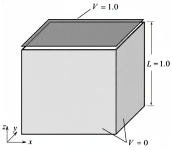
Figure 1. Model of an electrostatic cubic box.

The analytical solution of this equation is given by

$${\displaystyle V(x,y,z)=\sum _{m,\mathrm{odd}}\sum _{n,\mathrm{odd}}{a}_{mn}sin\left(m\pi x\right)sin\left(n\pi y\right)sinh\left(k_{mn}z\right)}$$

(29)

where

$${\displaystyle a_{mn}=\frac{16}{mn{\pi }^{2}sinh\left(k_{mn}\right)}}$$

(30)

$${\displaystyle k_{mn}=\pi \sqrt{\left(m^2+n^2\right)}.}$$

(31)

Applying the FDMO to benchmark electromagnetic problems, the 2D solution and corresponding error comparison shown in Figure 2a and Figure 2b, respectively, further demonstrate the advantages of FDMO in terms of precision and reliability. Beyond these benchmark results, the FDMO method shows strong potential for broader application in electromagnetic field problems. Specifically, the FDMO is well-suited for analyzing potential distribution in grounding systems, such as the evaluation of earth potential rise and touch or step voltages in substation grids. The method’s ability to handle various boundary conditions and heterogeneous soil properties allows for accurate modeling of real-world grounding scenarios. In summary, the FDMO method’s efficiency, versatility, and ease of implementation make it a valuable tool for both research and engineering applications in computational electromagnetics.

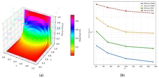
Figure 2. The 2D FDMO solution of potential distribution for the benchmark electromagnetic problem: (a) at the plane $y=0.5$ and (b) error norms.

3. Numerical Results

The electric field generated by the ground system within layered anisotropic soil is modeled through the scalar potential $\phi$, which adheres to Poisson’s equation and associated boundary constraints. In particular, the 3D domain of $\Omega$ is governed by Laplace equation, while the 2D boundary of $\Gamma$ is subject to specific conditions, such as those at the earth’s surface and at infinite distance. The mathematical formulation is expressed as follows:

• In the domain $\Omega$:

  $$\nabla ·\left(\right[\sigma ]\nabla \phi )=0$$

  (32)
• On the boundary $\Gamma$:

  $$\phi =0(r\to \infty ),{\displaystyle \frac{\partial \phi }{\partial n}}=0\left(\mathrm{in}\mathrm{earth}\mathrm{surface}\right).$$

  (33)

By employing the FDMO method to solve the governing Equation (32), we can determine both the electric potential $\phi$ and the corresponding current density $\sigma$ at any arbitrary point with coordinates $(x,y,z)$ in the computational domain as in Figure 3. This solution is obtained under the condition that the electrode achieves a specific voltage ${\phi }_{\Gamma }$, commonly referred to as the Ground Potential Rise (GPR), computed with respect to a far-field earth reference, thereby enabling a comprehensive analysis of the electromagnetic behavior in the grounding system.

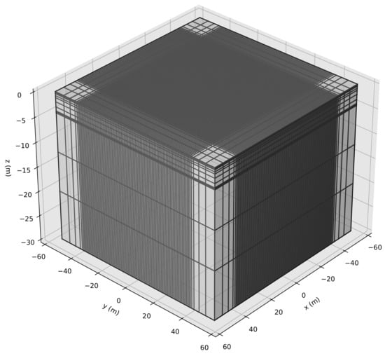
Figure 3. The model of the non-uniform FD mesh.

3.1. Case 1: Square-Shaped GS with Vertical Rods

The square-shaped GS was designed with dimensions of 70 m by 70 m [1]. Conductors were spaced at 7 m intervals, forming a 10 by 10 mesh configuration. The entire grid was installed at a depth of 0.8 m below the ground surface. Along the perimeter of the grid, vertical ground rods—each 3 m long and 10 mm in diameter—were driven into the soil at every second mesh interval, as illustrated in Figure 4a. The soil in the area has a resistivity of $\rho =400\Omega ·\mathrm{m}$. For applying the FDMO, this GS was modeled in the non-uniform FD mesh as in Figure 4b.

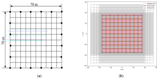
Figure 4. The square-shaped GS with vertical rods along its perimeter: (a) in IEEE Std 80^™ [1] and (b) square-shaped GS modeled in the non-uniform FD mesh.

The simulation outcomes for the potential distribution and the corresponding equipotential lines within the square-shaped GS are illustrated in Figure 5 and Figure 6, respectively. These visualizations provide an intuitive understanding of the electric field behavior across the GS domain. Furthermore, a detailed comparison between the FDMO and the FE solutions for the earth surface potential (ESP) is presented in Figure 7 and summarized in Table 1. The comparison shows a close agreement between the two numerical methods. Specifically, the maximum potential ${\phi }_{\max }$ obtained from FDMO is slightly higher (0.997 pu) than that from FEM (0.993 pu), while the minimum potential ${\phi }_{\min }$ predicted by FDMO is slightly lower (0.849 pu) compared to FEM (0.865 pu). Consequently, the maximum potential difference $\Delta {\phi }_{\max }$ calculated by FDMO is 0.148 pu, marginally greater than the 0.128 pu obtained by FEM. These minor discrepancies can be attributed to the different discretization schemes and numerical treatments employed by each method. Nevertheless, both FDMO and FEM demonstrate consistent and reliable results in capturing the potential distribution, with the FDMO method showing a slightly wider potential range. This confirms the validity and accuracy of the FDMO approach, establishing it as a robust and practical alternative to the well-established FE technique in grounding system studies.

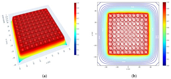
Figure 5. The FDMO solutions of potential distribution and equipotential lines for the square-shaped grounding system (GS): (a) 3D potential distribution and (b) equipotential lines on the ground surface.

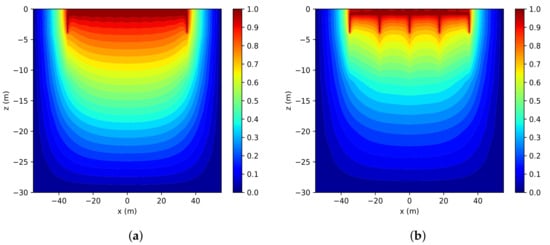
Figure 6. The distribution of equipotential lines of the square-shaped GS in soil: (a) at the center (along the x-axis) and (b) at the boundary.

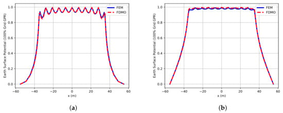
Figure 7. Comparison of the FDMO and FE solutions of the potential distributions in the square-shaped GS: (a) $x=y$ and (b) $y=0$.

Table 1. Comparison between FDMO and FE solutions for potential distribution in the square-shaped GS. ${\phi }_{\max }$ denotes the maximum electric potential on the ground surface. ${\phi }_{\min }$ denotes the minimum electric potential on the ground surface. $\Delta {\phi }_{\max }$ denotes the maximum potential difference across the ground surface.

Methods	${\mathit{\phi }}_{\mathbf{max}}$	${\mathit{\phi }}_{\mathbf{min}}$	$\mathbf{\Delta }{\mathit{\phi }}_{\mathbf{max}}$
FDMO	0.997 pu	0.849 pu	0.148 pu
FEM	0.993 pu	0.865 pu	0.128 pu

The computational results obtained using the proposed FDMO method demonstrate strong agreement with those derived from the IEEE Std 80^™–2013 [1] guidelines. As shown in Table 2, the values of maximum touch and step voltages predicted by FDMO closely match the standard values, with only minor deviations of 0.2% and 1.8% respectively. These small discrepancies confirm the accuracy and reliability of the FDMO approach for evaluating grounding system safety parameters, making it a robust alternative to conventional methods.

Table 2. Comparison between FDMO solution and IEEE Std 80^™ for touch and step voltages in the square-shape GS. $E_{\mathrm{touch}-\max }$ (%) denotes the maximum touch voltage, expressed as a percentage of the Ground Potential Rise (GPR) and $E_{\mathrm{step}-\max }$ (%) denotes the maximum step voltage, expressed as a percentage of the Ground Potential Rise (GPR).

Methods	${\mathit{E}}_{\mathbf{touch}-\mathbf{max}}$ (V)	${\mathit{E}}_{\mathbf{touch}-\mathbf{max}}$ (%)	${\mathit{E}}_{\mathbf{step}-\mathbf{max}}$ (V)	${\mathit{E}}_{\mathbf{step}-\mathbf{max}}$ (%)
FDMO	773.7	14.8	313.7	6.0
IEEE Std 80™	784.7	15.0	409.8	7.8

Figure 8 presents the computed touch and step voltage profiles at the center of the grounding grid. The results show the variation in surface potential and the corresponding voltage differences between two points, which are critical for assessing compliance with IEEE Std 80 safety limits.

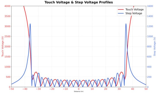
Figure 8. Touch and step voltage profiles at $y=0$.

3.2. Case 2: L-Shaped GS with Vertical Rods

The L-shaped GS covers an area of 4900 ${\mathrm{m}}^2$, with conductors arranged at 7 m intervals, resulting in a total of 100 mesh cells [1]. The grid was installed at a depth of $h=0.8$ m below ground level. Along the perimeter, vertical ground rods—each 3 m in length and 10 mm in diameter—were positioned at intervals corresponding to every two to three mesh cells, as illustrated in Figure 9a. The soil resistivity in the area is $\rho =400\Omega ·\mathrm{m}$. The soil volume considered for analysis measures 145 m × 110 m in area with a depth of 30 m. The same as with the square-shaped GS, the L-shaped GS is also modeled in the non-uniform FD mesh as in Figure 9b.

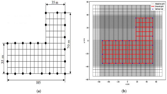
Figure 9. The L-shaped GS with vertical rods along its perimeter: (a) in IEEE Std 80^™ [1] and (b) L-shaped GS modeled in the non-uniform FD mesh.

The simulation results illustrating the potential distribution within the L-shaped grounding system are presented in Figure 10 and Figure 11. These figures provide both 3D and 2D visualizations, offering a comprehensive understanding of the voltage gradients and equipotential contours throughout the soil medium. Such detailed representations are crucial for assessing the grounding system’s performance and ensuring safety standards are met effectively.

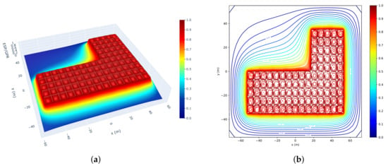
Figure 10. The FDMO solutions of the potential distribution and equipotential lines on the L-shaped GS: (a) 3D potentials and (b) equipotential lines on ground surfaces.

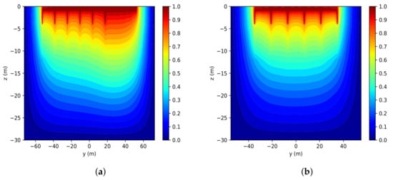
Figure 11. The distribution of equipotential lines of the L-shaped GS in soil: (a) at the center (along x-axis) and (b) at the boundary.

Figure 12 and Table 3 compare the potential distributions results obtained by the FDMO and FEM methods for the L-shaped GS. Both approaches yield very close values for the maximum and minimum potentials, with FDMO showing a slightly higher maximum potential and a slightly lower minimum potential than FEM. The difference in the maximum potential variation between the two methods is minimal, indicating that FDMO can accurately capture the potential behavior within the system. Overall, these findings validate the effectiveness of the FDMO technique as a reliable alternative to the conventional FEM approach in analyzing complex grounding configurations.

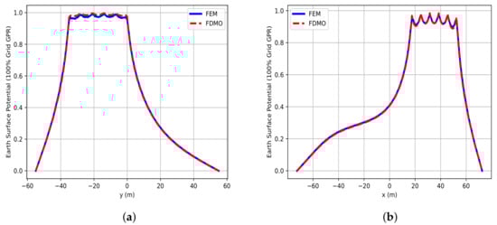
Figure 12. Comparison of the FDMO and FE solutions of potential distribution in the L-shaped GS: (a) $x=-18\mathrm{m}$ and (b) $y=18\mathrm{m}$.

Table 3. Comparison between FDMO and FEM solutions for potential distribution in the L-shaped grounding system.

Methods	${\mathit{\phi }}_{\mathbf{max}}$	${\mathit{\phi }}_{\mathbf{min}}$	$\mathbf{\Delta }{\mathit{\phi }}_{\mathbf{max}}$
FDMO	0.997 pu	0.850 pu	0.147 pu
FEM	0.993 pu	0.864 pu	0.129 pu

Table 4 presents a comparison of the maximum touch and step voltages calculated using the FDMO method and those specified by IEEE Std 80^™ [1]. The results show that the FDMO method yields values for both touch and step voltages that are in close alignment with the standard, with only minor deviations observed. Specifically, the maximum touch voltage calculated by FDMO is 762.9 V (14.7%), compared to 799.5 V (15.4%) from the IEEE standard. Similarly, the maximum step voltage from FDMO is 311.4 V (6.0%), while the standard gives 422.3 V (8.1%). These differences are relatively small and fall within acceptable engineering margins, confirming the reliability and accuracy of the FDMO approach for grounding system safety assessment. The close agreement between the FDMO results and those from the established IEEE standard demonstrates that the proposed method is a robust and effective tool for evaluating both touch and step voltages in practical applications.

Table 4. Comparison between FDMO solution and IEEE Std 80^™ for touch and step voltages in the L-shape GS.

Methods	${\mathit{E}}_{\mathbf{touch}-\mathbf{max}}$ (V)	${\mathit{E}}_{\mathbf{touch}-\mathbf{max}}$ (%)	${\mathit{E}}_{\mathbf{step}-\mathbf{max}}$ (V)	${\mathit{E}}_{\mathbf{step}-\mathbf{max}}$ (%)
FDMO	762.9	14.7	311.4	6.0
IEEE Std 80™	799.5	15.4	422.3	8.1

Similar to Figure 8, the touch and step voltage profiles of the L-shaped grounding system are presented in Figure 13. These profiles also exhibit noticeable variations in surface potential, reflecting changes in the potential gradient across the grounding grid area.

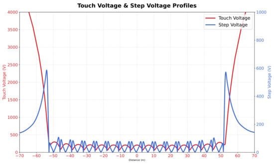
Figure 13. Touch and step voltage profiles at $y=-20\mathrm{m}$.

3.3. Case 3: Real-World GS

In this section, we investigated a real-world GS of the 22/110 kV–63 MVA Da Mi floating solar power substation which was developed in alignment with the government’s strategy to promote renewable energy sources. This project leveraged the Da Mi hydropower reservoir located in Ham Thuan Bac District, Binh Thuan Province, which was part of the Da Nhim–Ham Thuan–Da Mi hydropower complex managed by the Da Nhim–Ham Thuan–Da Mi Hydropower Joint Stock Company. The integration of this floating solar power plant with the existing hydropower infrastructure exemplified a forward-looking approach to sustainable energy development in the region.

The GS structure and equipment layout of this solar power substation, occupying an area of 65 m × 45 m, are depicted in Figure 14. The earth grid consists of galvanized steel wires with a diameter of 14 mm, complemented by galvanized steel rods (green dots) of the same diameter and 3 m in length. Additionally, steel rods (red dots) were used for a grounding enhancement material (GEM) well, which has a diameter of 120 mm and a depth of 30 m. All components were installed at a uniform depth of 0.8 m to ensure optimal performance and durability.

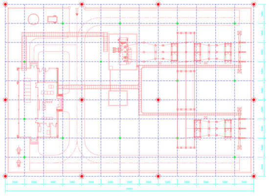
Figure 14. Real-world GS structure and equipment layout of the solar power substation in Vietnam.

This GS is characterized by key parameters critical to its performance under fault conditions. A phase-to-ground fault current of $I_f=8.42\mathrm{kA}$ is injected into the GS, with a fault duration of 0.5 s governing the step and touch voltage exposure. The surrounding soil exhibits an average resistivity of $\rho =300\Omega ·\mathrm{m}$, influencing the potential distribution across the system. Additionally, the total resistance of the grounding system, combined with the substation’s installation, is measured at $R_{GS}=0.49\Omega$, ensuring effective dissipation of fault currents and compliance with safety standards.

Applying the FDMO method to the real-world GS in Vietnam, we obtained the simulation results of the potential distribution and equipotential lines as shown in Figure 15 and Figure 16. The computation results of ESP obtained from the FDMO and FE methods for the real-world GS are compared in Figure 17a,b, and summarized in Table 5. The comparison highlights the strong agreement between the FDMO and FE methods in predicting the potential distribution within the real-world grounding system. While both methods provide reliable results, the FDMO approach demonstrates slightly more conservative estimations in terms of potential variations, which can be beneficial for ensuring safety margins in practical engineering applications. Additionally, the simplicity and computational efficiency of the FDMO method make it a valuable tool for rapid and accurate analysis, especially in scenarios where quick decision making is essential. This combination of accuracy, reliability, and efficiency underscores the practical advantages of the FDMO method as a competitive alternative to the traditional FE approach.

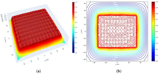
Figure 15. The FDMO solutions of the potential distribution and equipotential lines on the real-world GS: (a) 3D potentials and (b) equipotential lines on the ground surface.

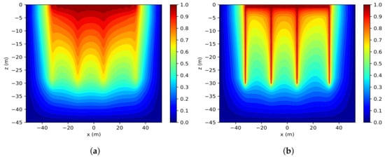
Figure 16. The distribution of equipotential lines of the real-world GS in soil: (a) at the center (along x-axis) and (b) at the boundary.

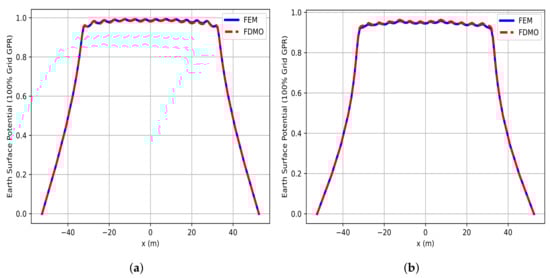
Figure 17. Comparison of the FDMO and FE solutions of the potential distributions in the real-world GS: (a) $x=y$ and (b) $y=0$.

Table 5. Comparison between FDMO and FEM solutions for potential distribution in the real-world GS.

Methods	${\mathit{\phi }}_{\mathbf{max}}$	${\mathit{\phi }}_{\mathbf{min}}$	$\mathbf{\Delta }{\mathit{\phi }}_{\mathbf{max}}$
FDMO	0.997 pu	0.895 pu	0.102 pu
FEM	0.997 pu	0.878 pu	0.119 pu

The comprehensive safety assessment of the grounding grid was conducted by calculating the maximum step and touch voltages using the finite difference method with optimization (FDMO) approach. The results were compared with the stringent limits prescribed by IEEE Std 80^™ [1], ensuring compliance with internationally recognized safety standards, as shown in Table 6. Specifically, the maximum touch voltage, $E_{\mathrm{touch}-\max ,\mathrm{FDMO}}=252.5\mathrm{V}$, is significantly lower than the IEEE permissible threshold of 621.7 V, providing a substantial safety margin of approximately 59.4%. Similarly, the maximum step voltage, $E_{\mathrm{step}-\max ,\mathrm{FDMO}}=74.3\mathrm{V}$, remains well below the allowable limit of 321.9 V for a 70 kg body weight, resulting in an impressive safety margin of about 76.9%. These findings confirm not only the robustness and reliability of the grounding grid design but also demonstrate the high accuracy and practical feasibility of the FDMO method in modeling complex grounding systems. Consequently, the grounding system is fully compliant with safety requirements, eliminating the need for further modifications and ensuring operational safety in high-voltage substations.

Table 6. Comparison between FDMO solution and IEEE Std 80^™ for touch and step voltages in the real-world GS.

Voltages	FDMO	IEEE Std 80™
$E_{\mathrm{touch}-\max }$ (V)	252.5	621.7
$E_{\mathrm{step}-\max }$ (V)	74.3	321.9

As shown in Figure 18, the computed potential distribution and step voltage along the line $y=0$ are illustrated for the real-world grounding system. These results are used to evaluate the safety performance of the grounding installation.

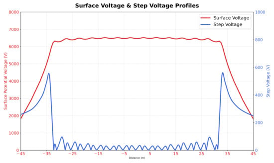
Figure 18. Potential and step voltage of the real-world GS along the line $y=0$.

4. Remark and Conclusions

Here, we can remark some main points as follows:

• Mathematical Formulation: The FDM is markedly simpler than other numerical approaches such as FEM, BEM, and MoM. The FDM offers a notably more straightforward mathematical formulation, which greatly facilitates its implementation, management, and programming. In particular, when applying the FDMO approach, 3D problems can be efficiently addressed through successive the Kronecker product of 1D operators, as formulated in Section 2.1.1. This approach proves especially advantageous for large-scale and geometrically complex problems, as well as for handling diverse types of boundary conditions.
• Accuracy and Cost-efficiency: As compared in Figure 2b, it can be observed that with only a few thousand discretization points in the computational domain, the FDMO solution achieves an error level comparable to or even lower than that of the FEM solution using hundreds of thousands of points. Therefore, the FDMO method can significantly reduce computational costs for practical large-scale and complex problems where extremely high accuracy is not required.
• Applicability: The FDMO method can be applied to a wide range of GS geometries, including square, rectangular, L-shaped, and real-world mesh configurations. With its computational efficiency and ease of implementation, this method can effectively support the design of high-voltage substation grounding systems. Moreover, it enables the evaluation of safety criteria such as earth resistance, and step and touch voltages, in compliance with IEEE standard, as discussed in Section 3.

In this study, we significantly advanced the FDMO algorithm, originally proposed in [13], by introducing a novel integration with a non-uniform FD mesh to tackle the 3D Poisson–Laplace equation governing electromagnetic problems in GS. This innovative approach is applied to complex geometries of IEEE Std 80^™ square and L-shape grid configurations and a real-world 220 kV high-voltage substation in Vietnam. The computed earth potential distributions, and touch and step voltages exhibit remarkable agreement with benchmarks from the FEM and IEEE Std 80^™ [1]. These results not only validate the FDMO method’s high accuracy and robustness but also highlight its practical utility in ensuring compliance with stringent safety standards for high-voltage substations. By offering a computationally efficient alternative to traditional numerical methods, the proposed approach reduces the reliance on resource-intensive simulations while maintaining precision, thereby addressing a critical need in power system engineering. The successful application to a real-world substation underscores the method’s versatility, paving the way for its adoption in diverse grounding system designs worldwide. Looking forward, this work lays a robust foundation for future research into adaptive mesh techniques, potential integration with real-time fault monitoring systems, and broader applications in optimizing grounding designs in power systems, ultimately enhancing the safety and reliability of electrical infrastructure.

Appendix A.1. Central Approximations

Using the central difference method, we approximated the first and second derivatives of the function f at the point $x_i$, based on the grid points $x_{i-1}$, $x_i$, and $x_{i+1}$, as given by (4) and (5), respectively. By applying Taylor series expansions of f about $x_i$ at the points $x_{i-1}$ and $x_{i+1}$, we derived the corresponding approximations as follows:

$$f_{i-1}=f_i+f_i^{\prime }(x_{i-1}-x_i)+{\displaystyle \frac{f_i^{″}}{2!}}{(x_{i-1}-x_i)}^2+O\left({(x_{i-1}-x_i)}^3\right)$$

(A1)

$$f_{i+1}=f_i+f_i^{\prime }(x_{i+1}-x_i)+{\displaystyle \frac{f_i^{″}}{2!}}{(x_{i+1}-x_i)}^2+O\left({(x_{i+1}-x_i)}^3\right).$$

(A2)

Let $h_1=x_i-x_{i-1}$ and $h_2=x_{i+1}-x_i$ represent the step sizes between consecutive grid points. By substituting the Taylor series expansions from (A1) and (A2) into the central difference formulas given by (4) and (5), we derived two systems of linear equations. Solving these systems yields the coefficients for the finite difference approximations of the first and second derivatives as the following:

$$\left[\begin{array}{ccc}1& 1& 1\\ -h_1& 0& -h_2\\ {\displaystyle \frac{h_1^2}{2}}& 0& {\displaystyle \frac{h_2^2}{2}}\end{array}\right]\left[\begin{array}{c}{\zeta }_1\\ {\zeta }_2\\ {\zeta }_3\end{array}\right]=\left[\begin{array}{c}0\\ 1\\ 0\end{array}\right]$$

(A3)

$$\left[\begin{array}{ccc}1& 1& 1\\ -h_1& 0& -h_2\\ {\displaystyle \frac{h_1^2}{2}}& 0& {\displaystyle \frac{h_2^2}{2}}\end{array}\right]\left[\begin{array}{c}{\xi }_1\\ {\xi }_2\\ {\xi }_3\end{array}\right]=\left[\begin{array}{c}0\\ 0\\ 1\end{array}\right].$$

(A4)

We can reformulate Equations (A3) and (A4) in matrix form as follows:

$$\mathbf{A}=\Psi \zeta ,$$

(A5)

$$\mathbf{B}=\Psi \xi .$$

(A6)

The unknown weighting coefficients in Equations (A5) and (A6) can be determined by solving the corresponding linear systems. Specifically, these coefficients were calculated by first setting up the system of equations. Once the system is established, the coefficients can be obtained using standard numerical techniques such as matrix inversion or iterative solvers. This approach ensures that the weighting coefficients are optimized for the given grid points, leading to accurate numerical approximations of the derivatives as the following:

$$\zeta ={\Psi }^{-1}\mathbf{A},$$

(A7)

$$\xi ={\Psi }^{-1}\mathbf{B}.$$

(A8)

Appendix A.2. Forward and Backward Approximations

Analogous to the central difference approximations outlined previously, we derived two systems of linear equations by applying forward difference approximations to the function f at the grid points $x_i$, $x_{i+1}$, and $x_{i+2}$. These systems were formulated by substituting the function values at these points into the forward difference formulas, resulting in equations that can be expressed in matrix form, as presented below. This approach established a systematic framework within the finite difference scheme, enabling efficient computation of the first and second derivatives. The method’s inherent flexibility allows it to be readily extended to complex geometries and diverse boundary conditions, making it a robust and versatile tool for numerically solving partial differential equations in various engineering applications as follows:

$$\left[\begin{array}{ccc}1& 1& 1\\ 0& -h_1& -h_2\\ 0& {\displaystyle \frac{h_1^2}{2}}& {\displaystyle \frac{h_2^2}{2}}\end{array}\right]\left[\begin{array}{c}{\zeta }_{1F}\\ {\zeta }_{2F}\\ {\zeta }_{3F}\end{array}\right]=\left[\begin{array}{c}0\\ 1\\ 0\end{array}\right]$$

(A9)

$$\left[\begin{array}{ccc}1& 1& 1\\ 0& -h_1& -h_2\\ 0& {\displaystyle \frac{h_1^2}{2}}& {\displaystyle \frac{h_2^2}{2}}\end{array}\right]\left[\begin{array}{c}{\xi }_{1F}\\ {\xi }_{2F}\\ {\xi }_{3F}\end{array}\right]=\left[\begin{array}{c}0\\ 0\\ 1\end{array}\right]$$

(A10)

and, similarly as above forward difference approximations, by substituting the function values at the points $x_i$, $x_{i-1}$, and $x_{i-2}$, we obtain the backward difference approximations at the selected points. The resulting equations can be compactly expressed in matrix form, as the following:

$$\left[\begin{array}{ccc}1& 1& 1\\ -h_1& -h_2& 0\\ {\displaystyle \frac{h_1^2}{2}}& {\displaystyle \frac{h_2^2}{2}}& 0\end{array}\right]\left[\begin{array}{c}{\zeta }_{1B}\\ {\zeta }_{2B}\\ {\zeta }_{3B}\end{array}\right]=\left[\begin{array}{c}0\\ 1\\ 0\end{array}\right]$$

(A11)

$$\left[\begin{array}{ccc}1& 1& 1\\ -h_1& -h_2& 0\\ {\displaystyle \frac{h_1^2}{2}}& {\displaystyle \frac{h_2^2}{2}}& 0\end{array}\right]\left[\begin{array}{c}{\xi }_{1B}\\ {\xi }_{2B}\\ {\xi }_{3B}\end{array}\right]=\left[\begin{array}{c}0\\ 0\\ 1\end{array}\right].$$

(A12)

Finally, we can reformulate Equations (A9)–(A12) as (A5) and (A6), and evaluate them using Equations (A7) and (A8) for the forward and backward difference approximations.

References

- IEEE-Std80; IEEE Guide for Safety in AC Substation Grounding. IEEE: New York, NY, USA, 2013.
- He, J.; Zeng, R.; Zhang, B. Methodology and Technology for Power System Grounding; John Wiley & Sons: Hoboken, NJ, USA, 2012. [Google Scholar]
- Meliopoulis, A.S. Power System Grounding and Transients: An Introduction; Routledge: Abingdon, UK, 2017. [Google Scholar]
- Sverak, J.G. Progress in step and touch voltage equations of ANSI/IEEE Std 80-historical perspective. IEEE Trans. Power Deliv. 1998, 13, 762–767. [Google Scholar] [CrossRef]
- Trlep, M.; Hamler, A.; Hribernik, B. The analysis of complex grounding systems by FEM. IEEE Trans. Magn. 1998, 34, 2521–2524. [Google Scholar] [CrossRef]
- Kumar, A.; Rahi, O. Enhancing Substation Earthing System: A Finite Element Method For Minimizing Ground Resistance and Analyzing Electric Potential and Temperature Distribution. In Proceedings of the 2025 First International Conference on Advances in Computer Science, Electrical, Electronics, and Communication Technologies (CE2CT), Nainital, India, 21–22 February 2025; pp. 354–359. [Google Scholar]
- Colominas, I.; Navarrina, F.; Casteleiro, M. Analysis of transferred earth potentials in grounding systems: A BEM numerical approach. IEEE Trans. Power Deliv. 2005, 20, 339–345. [Google Scholar]
- Colominas, I.; Navarrina, F.; Casteleiro, M. Numerical simulation of transferred potentials in earthing grids considering layered soil models. IEEE Trans. Power Deliv. 2007, 22, 1514–1522. [Google Scholar] [CrossRef]
- Colominas, I.; Paris, J.; Guizan, R.; Navarrina, F.; Casteleiro, M. Numerical modeling of grounding systems for aboveground and underground substations. IEEE Trans. Ind. Appl. 2015, 51, 5107–5115. [Google Scholar] [CrossRef]
- Guizán, R.; Colominas, I.; París, J.; Couceiro, I.; Navarrina, F. Numerical analysis and safety design of grounding systems in underground compact substations. Electr. Power Syst. Res. 2022, 203, 107627. [Google Scholar] [CrossRef]
- Trlep, M.; Hamler, A.; Jesenik, M.; Stumberger, B. The FEM-BEM analysis of complex grounding systems. IEEE Trans. Magn. 2003, 39, 1155–1158. [Google Scholar] [CrossRef]
- Berberovic, S.; Haznadar, Z.; Stih, Z. Method of moments in analysis of grounding systems. Eng. Anal. Bound. Elem. 2003, 27, 351–360. [Google Scholar] [CrossRef]
- Zaman, M.A. Numerical Solution of the Poisson Equation Using Finite Difference Matrix Operators. Electronics 2022, 11, 2365. [Google Scholar] [CrossRef]
- Parreira, G.F.; Silva, E.J.; Fonseca, A.R.; Mesquita, R.C. The element-free Galerkin method in three-dimensional electromagnetic problems. IEEE Trans. Magn. 2006, 42, 711–714. [Google Scholar] [CrossRef]
- Zhang, Y.; Shao, K.; Guo, Y.; Zhu, J.; Xie, D.; Lavers, J. An improved multiquadric collocation method for 3-D electromagnetic problems. IEEE Trans. Magn. 2007, 43, 1509–1512. [Google Scholar] [CrossRef][Green Version]
- Vu, P.; Fasshauer, G. Application of two radial basis function-pseudospectral meshfree methods to three-dimensional electromagnetic problems. IET Sci. Meas. Technol. 2011, 5, 206–210. [Google Scholar] [CrossRef]
Disclaimer/Publisher’s Note: The statements, opinions and data contained in all publications are solely those of the individual author(s) and contributor(s) and not of MDPI and/or the editor(s). MDPI and/or the editor(s) disclaim responsibility for any injury to people or property resulting from any ideas, methods, instructions or products referred to in the content. |
© 2025 by the authors. Licensee MDPI, Basel, Switzerland. This article is an open access article distributed under the terms and conditions of the Creative Commons Attribution (CC BY) license (https://creativecommons.org/licenses/by/4.0/).