Numerical Modeling and Analysis of Shadow Flicker Using Solar Path Functions for Enhanced Predictive Accuracy

Abstract

Shadow flicker caused by wind turbine blades passing through sunlight can significantly affect nearby residential buildings, raising environmental and regulatory concerns in wind farm development. The accurate assessment of shadow flicker exposure is critical for compliance and minimizing community impacts. We present a novel method for accurately determining the exposure of shadow flicker from wind turbines on residential buildings, addressing a key regulatory concern in wind farm planning. Current simulation techniques rely on discrete sampling of solar positions, resulting in potential inaccuracies tied to sampling resolution. Our proposed approach models shadow flicker as a continuous function and applies numerical minimization and numerical root finding to compute the duration of exposure. Our evaluation proves that this method achieves a superior balance between precision and computational efficiency, significantly improving existing techniques.

1. Introduction

Many European states are navigating the transition to renewable energies with wind energy playing a significant role. Shadow flicker (SF) is a phenomenon where the rotating blades of a wind turbine cast moving shadows that create a flickering effect on their surroundings and potentially on residential buildings. This effect, while generally considered to have no direct health impacts, can cause discomfort or annoyance if the flicker frequency exceeds certain thresholds [1,2]. To mitigate this, many jurisdictions impose strict regulations limiting the amount of SF exposure that residents can experience. These regulations include both annual and daily exposure limits.

Current simulation tools, such as windPRO (Version 4.1) [3] and WindFarmer (Version 1.6.2) [4], model the solar position at discrete time points, typically with a resolution between one and three minutes [5,6,7]. This approach inevitably leads to a resolution-dependent discretization error in predicting SF exposure. As a result, a user of this method has the dilemma to balance between a high resolution, resulting in a low discretization error but high running time, and a low resolution, resulting in low running time but high discretization error. With a too low resolution, we potentially misestimate the duration of SF too strongly and thus falsely discard or allow turbine positions when trying to comply with regulations.

1.1. Problem Description

In this paper, we propose a novel method for the following problem: for a specific day, a wind turbine with known specifications and fixed position, and a receiver position (e.g., of a residential building), find the amount of time during which the receiver experiences SF from the wind turbine on the given day.

1.2. Related Work

Renewable energy, especially wind farms, have received significant attention from the research communities in the last two decades. Most closely related to our work are the modeling, simulation, and layout optimization of wind farms. Wind turbine wake models, describing the wind turbulence and speed reduction caused by wind turbines in their downstream region, have been researched extensively in the past few decades [8]. Simulators embed those wake models to estimate the efficieny of wind farms and provide the basis for wind farm layout optimization [9,10].

Wind farm site suitability is yet another related field of research investigating the suitability of sites with respect to potential wind farms [11]. SF has been considered in some works for site suitability and layout optimization, but the method used was always the discretization approach and was never described in detail. We are not aware of any literature that addresses the topic of SF modeling and computation in particular. The above-described discretization method has been accepted as the standard and has not been questioned.

The above approaches have been implemented in different wind farm simulation tools. To the best of our knowledge, all tools that support SF simulation, including windPRO (Version 4.1) [3] and WindFarmer (Version 1.6.2) [4], compute SF emissions based on discrete samples of the solar position.

1.3. Core Idea

We propose a novel approach, which overcomes the aforementioned limitations of utilizing discretization. We model shadow flicker as a continuous phenomenon over time to enable the application of minimization and real root-finding algorithms for computing the duration of exposure. However, the continuous model for the sun’s position is too complex for analytical methods. Therefore, we side-step to numerical methods, namely numerical minimization and numerical root finding, which only require executability for the continuous model. As executing the model is fast, the new method can calculate SF durations quickly and with high precision. Although the numerical methods introduce an error, it is possible to specify the maximum error of these methods in advance. Our new method thus offers an improved balance between precision and computational efficiency.

1.4. Contributions

With this paper, we make the following contributions:

• We propose a new SF approximation method that models SF as a continuous function of time and has an improved balance between precision and computational efficiency.
• We provide an implementation of the proposed method.
• We experimentally evaluate our new method and compare the results to those of the currently used discretization method.

1.5. Outline

The rest of this paper is structured as follows. We start in Section 2 with an overview of the methodology used in this paper, providing an abstract description of the contents of the remaining sections. In Section 3, we describe the parameters which we use to specify our continuous SF model. We describe the continuous models for the sun position in Section 4 and for the SF function in Section 5. Based on these continuous models, in Section 6, we present our novel method to compute the SF duration. Our method makes certain assumptions, whose validity we discuss in Section 7. We present the experimental results in Section 8 and conclude the presentation with some remarks and ideas for possible future work in Section 9.

2. Methodology

In this section, we present an overview of the methodology that we use in this paper to solve the problem presented in Section 1. An illustration is depicted in Figure 1.

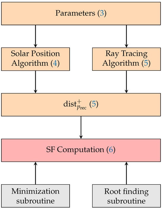
Figure 1. Schematic overview of the structure and methodology of this paper. The corresponding sections are referenced in brackets.

The core of our new approach is the SF computation, which is presented in Section 6. However, as this method is quite complex, we first build foundations in Section 3, Section 4 and Section 5. In Section 3, we introduce all the parameters that we need throughout this paper. These parameters are then used in the Section 4 and Section 5. In Section 4, we introduce the continuous solar position algorithm that we used in our work to determine the position of the sun at a given time point on a certain day. In Section 5, we continue with presenting our ray tracing algorithm to calculate whether a given receiver experiences SF from a given wind turbine for a specific time of a day. We remark that the ray tracing algorithm uses the solar position algorithm to compute the solar position at the time point of interest, but the solar position algorithm and the ray tracing algorithm are not further related. Using both the solar position algorithm and the ray tracing algorithm, we complete Section 5 by defining the function ${\mathrm{dist}}_{p_{\mathrm{rec}}}^{+}$ that encodes whether SF occurs at a given time on a certain day. In Section 6, we then finally combine all previous results to present a novel approach to the SF computation problem. Our novel approach uses external, numerical subroutines for minimization and root finding on the previously derived function ${\mathrm{dist}}_{p_{\mathrm{rec}}}^{+}$.

In Section 7, we discuss the correctness of our algorithm, which is supported by our validation in Section 8. Finally, we draw a conclusion in Section 9.

3. Parameters

The problem described in Section 1 is parametric in multiple variables. In this section, we introduce the variables used. Some of these variables are illustrated in Figure 2. The problem is 3-dimensional and defined for a single day d. In our calculations, we use 3-dimensional Cartesian coordinates and polar coordinates. By $p_{\mathrm{rec}}$ and $p_{\mathrm{tur}}$, we refer to the Cartesian coordinates of the receiver and the wind turbine hub, respectively. The wind turbine’s radius is $r_{\mathrm{tur}}$, whereas $n_{\mathrm{tur}}$ is a Cartesian vector pointing in the direction the turbine’s rotor faces. The sun position is defined by $\psi$, $\theta$, and $\zeta$ in polar coordinates, which can be translated to Cartesian coordinates resulting in $n_{\mathrm{sun}}$. The solar hour angle $\omega$, the solar declination $\delta$, and the receiver’s latitude $\lambda$ are all necessary to calculate the sun direction. In the following, we provide a comprehensive list of these variables.

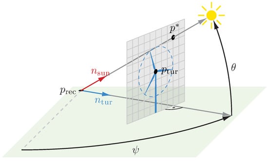
Figure 2. Illustration of the ray-tracing algorithm.

d 

$=[t_{\mathrm{start}},t_{\mathrm{end}}]$ specifies the day of interest with its start and end points in time.

$p_{\mathrm{tur}}$

$={(0,0,0)}^{⊺}\in {\mathbb{R}}^3$ is the position of the the center of the wind turbine’s hub. It is defined as the origin of the coordinate system used.

$p_{\mathrm{rec}}$

$\in {\mathbb{R}}^3$ is the receiver position for which we calculate its experienced SF duration.

$r_{\mathrm{tur}}$

$\in \mathbb{R}$ is the wind turbine’s rotor radius.

$\psi \left(t\right)$

$\in [0°,360°]$ is the solar azimuth angle at time $t\in d$, which tracks the sun’s (horizontal) movement along the horizon from the receiver’s perspective.

$\theta \left(t\right)$

$\in [-90°,90°]$ is the solar elevation angle at time $t\in d$, describing the sun’s vertical angle from the receiver’s perspective.

$\zeta \left(t\right)$

$\in [0°,180°]$ is the solar zenith angle at time $t\in d$; it is complementary to the elevation angle $\theta$ as it describes the vertical position of the sun relative to the solar zenith (in contrast to the horizon). It is defined as $\zeta \left(t\right)=90°-\theta \left(t\right)$.

$\omega \left(t\right)$

$\in [-180°,180°]$ is a monotonous non-linear function defining the solar hour angle at time $t\in d$ and ranges from $-180°$ at solar midnight to $180°$, approximately 24 h later, at solar midnight of the following day.

$\delta \left(t\right)$

$\in [-23.45°,23.45°]$ is the solar declination at time $t\in d$ and describes the angle between the earth’s equatorial plane and the sun direction. For a single day, some solar position algorithms assume it to be constant.

$\lambda$

$\in [-90°,90°]$ is the receiver’s latitude on the earth.

$n_{\mathrm{tur}}\left(t\right)$

$\in {\mathbb{R}}^3$ is the normal vector with the direction that the turbine’s rotor faces at time $t\in d$. In accordance with most regulations, we make the (worst-case) assumption that the turbine is facing the sun. Therefore, $n_{\mathrm{tur}}\left(t\right)$ is defined by the azimuth angle $\psi \left(t\right)$.

$n_{\mathrm{sun}}\left(t\right)$

$\in {\mathbb{R}}^3$ is the normal vector in the direction from the receiver to the sun at time $t\in d$. It is defined by the azimuth $\psi \left(t\right)$ and the elevation $\theta \left(t\right)$.

In the edge case of $\theta \left(t\right)\in \{-90°,90°\}$, meaning that the sun is exactly above or below the receiver, $n_{\mathrm{tur}}\left(t\right)$ is undefined. However, in this case, SF cannot occur, and our method handles this edge case using case distinctions. In the following descriptions, we assume $\theta \left(t\right)\notin \{-90°,90°\}$.

We assume furthermore a fixed time point $t\in d$ and write for the sake of readability $\psi ,\theta ,\dots$ instead of $\psi \left(t\right),\theta \left(t\right),\dots$ when we apply the functions to this fixed time point t. As further notation, we use indices to refer to vector components; e.g., we refer to the components of $v={(a,b,c)}^{⊺}$ as $v_1=a,v_2=b$ and $v_3=c$.

4. Solar Position

As sketched in the introduction, we need a continuous sun position model for our new method to compute SF. To calculate the sun’s position at time t, three parameters have to be provided:

$\lambda$

is a known constant as it is the receiver’s latitude on the earth.

$\delta \left(t\right)$

is computed using existing libraries; we consider it constant within a single day.

$\omega \left(t\right)$

is computed using existing libraries.

With these three values, it is then possible to first compute the elevation angle $\theta$, and then, using the close relation between $\theta$ and $\zeta$, the azimuth angle $\psi$:

$$\begin{array}{c}\hfill sin\left(\theta \right)=sin\left(\delta \right)sin\left(\lambda \right)+cos\left(\delta \right)cos\left(\lambda \right)cos\left(\omega \right)sin\left(\psi \right)=-{\displaystyle \frac{sin\left(\omega \right)cos\left(\delta \right)}{sin\left(\zeta \right)}}.\end{array}$$

(1)

The calculation of the solar hour angle $\omega$ is very complex because the sun’s and the earth’s position are affected by multiple dynamic factors. Therefore, different approximation algorithms with varying complexity and precision have been developed. The Solar Position Algorithm by Meeus [12], as detailed by Reda and Andreas [13], is widely employed in scientific computations where high precision is crucial, offering uncertainties as low as $\pm 0.0003°$ for both the solar azimuth and elevation angles. We have used this algorithm for the implementation in this paper.

5. Ray Tracing

In this section, assuming a given sun position $(\psi ,\theta )$ at time point t, we show how we can determine whether the receiver is shadowed by the wind turbine. This calculation is called ray tracing.

The standard method, illustrated in Figure 2, is to draw a line between the receiver and the sun and then check whether it intersects with the turbine rotor. More formally, using the position of the sun $(\psi ,\theta )$, we can calculate the vectors $n_{\mathrm{sun}}$ and $n_{\mathrm{tur}}$ as

$$n_{\mathrm{sun}}=\left(\begin{array}{c}cos\left(\theta \right)cos\left(\psi \right)\\ cos\left(\theta \right)sin\left(\psi \right)\\ sin\left(\theta \right)\end{array}\right)\mathit{respectively}{n}_{\mathrm{tur}}=\left(\begin{array}{c}cos\left(\psi \right)\\ sin\left(\psi \right)\\ 0\end{array}\right).$$

(2)

To calculate whether the line between the receiver and the sun intersects with the turbine rotor, we use the turbine position $p_{\mathrm{tur}}$ and span a plane with normal vector $n_{\mathrm{tur}}$ (see Figure 2). We then calculate this plane’s intersection $p^{\ast }$ with the line between the sun and the receiver. If the distance between $p^{\ast }$ and $p_{\mathrm{tur}}$ is smaller or equal to the rotor radius, then the receiver is shadowed; otherwise, it is not.

As the vector $p^{\ast }-p_{\mathrm{tur}}$ lies on the plane with normal vector $n_{\mathrm{tur}}$, we know that $p^{\ast }-p_{\mathrm{tur}}$ and $n_{\mathrm{tur}}$ are orthogonal, and we can deduce

$$0=(p^{\ast }-p_{\mathrm{tur}})·n_{\mathrm{tur}}=p^{\ast }·n_{\mathrm{tur}},$$

(3)

where the second equality holds because the turbine position $p_{\mathrm{tur}}$ is defined as the origin. We further know that $p^{\ast }$ lies on the line between the receiver and the sun, meaning

$$p^{\ast }=p_{\mathrm{rec}}+d·n_{\mathrm{sun}}$$

(4)

for some $d\in \mathbb{R}$. Inserting Equation (4) into Equation (3) yields

$$0=(p_{\mathrm{rec}}+d·n_{\mathrm{sun}})·n_{\mathrm{tur}}\Rightarrow d=-{\displaystyle \frac{p_{\mathrm{rec}}·n_{\mathrm{tur}}}{n_{\mathrm{sun}}·n_{\mathrm{tur}}}}.$$

(5)

Note that $n_{\mathrm{sun}}·n_{\mathrm{tur}}\in \mathbb{R}\setminus \left\{0\right\}$ as we have excluded the case $\theta \in \{-90,90\}$ in Section 3. Finally, we insert Equation (5) into Equation (4) to obtain

$$p^{\ast }=p_{\mathrm{rec}}-\left({\displaystyle \frac{p_{\mathrm{rec}}·n_{\mathrm{tur}}}{n_{\mathrm{sun}}·n_{\mathrm{tur}}}}\right)·n_{\mathrm{sun}}.$$

(6)

To determine whether the position on the ground $p_{\mathrm{rec}}$ experiences shadow flicker, we check whether the distance between $p^{\ast }$ and $p_{\mathrm{tur}}$ is smaller than the rotor radius $r_{\mathrm{tur}}$. In this case, the rotor intersects the line between the receiver and the sun. As we defined $p_{\mathrm{tur}}$ as the origin, it is sufficient to check $\parallel p^{\ast }{\parallel }_2\le r_{\mathrm{tur}}$. We thus define the distance function as

$${\mathrm{dist}}_{p_{\mathrm{rec}}}(\psi ,\theta ):={∥p^{\ast }∥}_2.$$

(7)

The condition ${\mathrm{dist}}_{p_{\mathrm{rec}}}(\psi ,\theta )<r_{\mathrm{tur}}$ may also be fulfilled for negative $\theta$ if the receiver is between the rotor and the sun, as illustrated in Figure 3. Thus, $\theta \ge 0$ is an additional necessary condition for SF. To cover this condition, if $\theta <0$, then before executing further computations, we set $\theta$ to 0. Furthermore, in order to guarantee $\parallel p^{\ast }{\parallel }_2>r_{\mathrm{tur}}$ for $\theta =0$, we assume that the receiver’s altitude is never higher than the lowest point of the rotor, meaning $p_{\mathrm{tur},3}-r_{\mathrm{tur}}>p_{\mathrm{rec},3}$. Formally, we define

$${\mathrm{dist}}_{p_{\mathrm{rec}}}^{+}\left(t\right)=\left\{\begin{array}{cc}{\mathrm{dist}}_{p_{\mathrm{rec}}}(\psi \left(t\right),\theta \left(t\right))-r_{\mathrm{tur}}\hfill & \theta \left(t\right)\ge 0\hfill \\ {\mathrm{dist}}_{p_{\mathrm{rec}}}(\psi \left(t\right),0)-r_{\mathrm{tur}}\hfill & \mathrm{otherwise}.\hfill \end{array}\right..$$

(8)

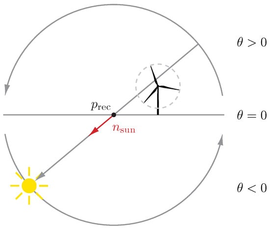
Figure 3. Special case in which ${\mathrm{dist}}_{p_{\mathrm{rec}}}(\psi ,\theta )<r_{\mathrm{tur}}$ for $\theta <0$.

The above definition resets the elevation angle $\theta$ to zero as soon as it would fall below zero. Furthermore, it shifts ${\mathrm{dist}}_{p_{\mathrm{rec}}}$ by $-r_{\mathrm{tur}}$. We can therefore conclude that SF occurs at t if and only if ${\mathrm{dist}}_{p_{\mathrm{rec}}}^{+}\left(t\right)\le 0$. Algorithm 1 shows the pseudocode to compute ${\mathrm{dist}}_{p_{\mathrm{rec}}}^{+}\left(t\right)$.

We remark that if we would apply discretization, then in case of $\theta <0$, we could directly report no SF. However, as we will see in the next section, we exploit the continuity of the distance function, which we maintain by pulling negative elevation angles to zero.

Algorithm 1: Pseudocode of the ${\mathrm{dist}}_{p_{\mathrm{rec}}}^{+}$ function

Input: t: time point for which to calculate ${\mathrm{dist}}_{p_{\mathrm{rec}}}^{+}$                $p_{\mathrm{rec}}$: receiver position  1              $r_{\mathrm{tur}}$: turbine rotor radius  2  Output: ${\mathrm{dist}}_{p_{\mathrm{rec}}}^{+}\left(t\right)$: distance as defined in Equation (8)  3  $\omega$:= calculate the hour angle at t according to Meeus [12];  4  $\psi$:= calculate the azimuth angle at t according to Equation (1);  5  $\theta$:= calculate the elevation angle at t according to Equation (1);  6  if $(\theta <0)$ then $\theta :=0$;  7  $n_{\mathrm{sun}}:={(cos\left(\theta \right)cos\left(\psi \right),cos\left(\theta \right)sin\left(\psi \right),sin\left(\theta \right))}^{⊺}$;  8  $n_{\mathrm{tur}}$:= ${(cos\left(\psi \right),sin\left(\psi \right),0)}^{⊺}$;  9  $p^{\ast }$:= $p_{\mathrm{rec}}-\left({\displaystyle \frac{p_{\mathrm{rec}}·n_{\mathrm{tur}}}{n_{\mathrm{sun}}·n_{\mathrm{tur}}}}\right)·n_{\mathrm{sun}}$; 10 return ${∥p^{\ast }∥}_2-r_{\mathrm{tur}}$;

6. Shadow Flicker Computation

In this section, we show how to compute the amount of time during which the receiver at $p_{\mathrm{rec}}$ experiences SF on day $d=[t_{\mathrm{start}},t_{\mathrm{end}}]$ from a wind turbine with hub position $p_{\mathrm{tur}}$ and rotor radius $r_{\mathrm{tur}}$.

We first define an indicator function ${\mathbb{1}}_{SF}:d\to \{0,1\}$ with

$${\mathbb{1}}_{SF}\left(t\right)=\left\{\begin{array}{c}10<\theta \left(t\right)<90°\wedge {\mathrm{dist}}_{p_{\mathrm{rec}}}^{+}\left(t\right)\le 0\hfill \\ 0\mathrm{otherwise}\hfill \end{array}\right.$$

(9)

for all $t\in d$. Then, the SF duration T for the day d is naturally defined by

$$T={\int }_{t_{\mathrm{start}}}^{t_{\mathrm{end}}}{\mathbb{1}}_{SF}\left(t\right)dt.$$

(10)

Note that this function assumes that no clouds prevent SF and that the turbine is operating continuously. As regulations often assume this (worst-case) scenario, we do the same in this paper.

It is infeasible to integrate ${\mathbb{1}}_{SF}$ analytically, as it depends on the functions for the azimuth angle $\psi$, the elevation angle $\theta$, and thereby on the function for the hour angle $\omega$, for which there is no analytically integrable model available.

In Section 6.1, we first present the traditional method that is currently used, which approximates T through discretization. We present our new approach in Section 6.2.

6.1. Discretization

Instead of calculating Equation (10) directly, the standard approach discretizes for some $n\in \mathbb{N}$ the day d to $n+1$ sample time points through $\Delta t:={\displaystyle \frac{t_{\mathrm{end}}-t_{\mathrm{start}}}{n}}$ and $t_i=t_{\mathrm{start}}+i·\Delta t$ for $i=0,\dots ,n$. Assuming the continuity of (non-)exposure between two samples, we can approximate T with

$$T\approx \Delta t·\sum _{i=0}^{n-1}{\mathbb{1}}_{SF}\left(t_i\right).$$

(11)

Note that this function now only requires knowing $\psi$ and $\theta$ at specific points in time, substantially reducing the complexity of the calculation. Furthermore, note that

$$T=\underset{n\to \infty }{lim}\Delta t·\sum _{i=0}^{n-1}{\mathbb{1}}_{SF}\left(t_i\right).$$

(12)

The above method, using discretization, inevitably suffers from the discretization error that scales with the sampling distance $\Delta t$. Improving precision introduces computational overhead. In the next section, we therefore present our novel approach that does not rely on discretization.

6.2. Continuous Shadow Model

Now, we are ready to present our novel approach to calculate the SF duration for a single day. A flow chart diagram of the standard case of our algorithm is shown in Figure 4; the pseudocode of the algorithm is shown in Algorithm 2.

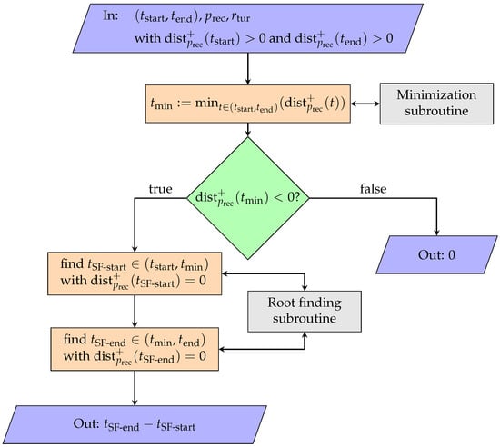
Figure 4. Flow chart diagram for the standard case of our method presented in Section 6.2 to calculate the SF duration of day d. The corresponding pseudocode is shown in Algorithm 2. Note that for simplicity, the flow chart diagram only covers the first case of the algorithm. Further note the embedded numerical methods for minimization and root finding.

We distinguish between days on which SF occurs and on which SF does not occur. The function ${\mathrm{dist}}_{p_{\mathrm{rec}}}^{+}$ is defined such that SF occurs at time t if and only if ${\mathrm{dist}}_{p_{\mathrm{rec}}}^{+}\left(t\right)\le 0$. If ${\mathrm{dist}}_{p_{\mathrm{rec}}}^{+}\left(t\right)$ does not become negative during the whole day, then SF exposure happens at most at a single point in time (namely, if ${\mathrm{dist}}_{p_{\mathrm{rec}}}^{+}$ obtains 0 for one moment), which we neglect. Therefore, if ${\mathrm{dist}}_{p_{\mathrm{rec}}}^{+}\left(t\right)\ge 0$ for all $t\in d$, then we conclude SF freedom on day d.

Because $r_{\mathrm{tur}}$ and $p_{\mathrm{rec}}$ are fixed constants and, as mentioned in Section 3, we handle the case $\psi =90°$ separately, ${\mathrm{dist}}_{p_{\mathrm{rec}}}^{+}$ is a continuous function over d. To determine whether there is a value $t_{\min }\in d$ with ${\mathrm{dist}}_{p_{\mathrm{rec}}}^{+}\left(t_{\min }\right)<0$, we minimize ${\mathrm{dist}}_{p_{\mathrm{rec}}}^{+}\left(t\right)$ over $t\in d$ with the help of a numerical optimization algorithm. In our implementation, we use Brent’s numerical minimization algorithm [14], which itself is based on Dekker’s algorithm. If Brent’s minimization algorithm does not find $t_{\min }$ with ${\mathrm{dist}}_{p_{\mathrm{rec}}}^{+}\left(t_{\min }\right)<0$, we assume that such a $t_{\min }$ does not exist and the receiver does not experience any SF on that day. Although it is theoretically possible that Brent’s minimization does not find such a $t_{\min }$ even if it exists, we argue in Section 7.2 that it is nonetheless sensible to make this assumption.

Assume in the following that the minimum is negative, i.e., SF occurs during the day. Remember that we neglect the cases when clouds prevent SF or when the turbine does not operate. For days on which SF occurs, we first explain the standard case when SF occurs continuously within one single connected interval $[t_{\mathrm{SF}-\mathrm{start}},t_{\mathrm{SF}-\mathrm{end}}]$ during the day. Later, in Section 6.2.1, we will explain how to handle the seldom case, which is possible only near the north or south pole of the Earth, when the day starts or ends with SF because midnight falls into an SF interval. In very rare cases, SF may also occur during two disconnected time intervals within one day if the minimum of ${\mathrm{dist}}_{p_{\mathrm{rec}}}^{+}$ is at a timepoint $t_{\min }$ very close to the beginning or to the end of the day. Thus, if $t_{\min }$ is found near $t_{\mathrm{start}}$ or $t_{\mathrm{end}}$, then in our implementation we use the numerical minimization algorithm for a second time at the other end of the day to check whether this case applies. For simplicity, this case is not covered in our main Algorithm 2. Due to the complexity of the models, we cannot provide a formal proof that no other than one of the above cases can apply. However, in addition to the experimental results which all confirm validity, in Section 7.1, we provide additional arguments as to why our assumption is reasonable.

We first consider the standard case, when there is no SF at the beginning and at the end of the day $d=[t_{\mathrm{start}},t_{\mathrm{end}}]$, i.e., ${\mathrm{dist}}_{p_{\mathrm{rec}}}^{+}\left(t_{\mathrm{start}}\right)>0$ and ${\mathrm{dist}}_{p_{\mathrm{rec}}}^{+}\left(t_{\mathrm{end}}\right)>0$. As mentioned, a flow chart diagram for this standard case is shown in Figure 4. We remind that the function ${\mathrm{dist}}_{p_{\mathrm{rec}}}^{+}$ is continuous. Because ${\mathrm{dist}}_{p_{\mathrm{rec}}}^{+}\left(t_{\mathrm{start}}\right)>0$, ${\mathrm{dist}}_{p_{\mathrm{rec}}}^{+}\left(t_{\min }\right)<0$ and ${\mathrm{dist}}_{p_{\mathrm{rec}}}^{+}\left(t_{\mathrm{end}}\right)>0$ for $t_{\mathrm{start}}<t_{\min }<t_{\mathrm{end}}$, from the continuity of the function ${\mathrm{dist}}_{p_{\mathrm{rec}}}^{+}$ we conclude that there is a maximal SF emmission interval $t_{\min }\in [t_{\mathrm{SF}-\mathrm{start}},t_{\mathrm{SF}-\mathrm{end}}]\subseteq (t_{\mathrm{start}},t_{\mathrm{end}})$ with ${\mathrm{dist}}_{p_{\mathrm{rec}}}^{+}\left(t_{\mathrm{SF}-\mathrm{start}}\right)={\mathrm{dist}}_{p_{\mathrm{rec}}}^{+}\left(t_{\mathrm{SF}-\mathrm{end}}\right)=0$. As argued above and in Section 7.1, we assume that this is the only interval in d with SF emmission, and we conclude that

$$T={\int }_{t_{\mathrm{start}}}^{t_{\mathrm{end}}}{\mathbb{1}}_{SF}\left(t\right)dt=\left\{\begin{array}{cc}{t}_{\mathrm{SF}-\mathrm{end}}-t_{\mathrm{SF}-\mathrm{start}}\hfill & \mathrm{if}\mathrm{SF}\mathrm{occurs}\hfill \\ 0\hfill & \mathrm{otherwise}.\hfill \end{array}\right.$$

(13)

We identify the endpoints of the only SF interval during d as the only two zeros of ${\mathrm{dist}}_{p_{\mathrm{rec}}}^{+}$ within d. As our model for the function ${\mathrm{dist}}_{p_{\mathrm{rec}}}^{+}$ is too complex for algebraic solutions, we use it as an executable model and sidestep to iterative numerical methods. In our implementation, Brent’s numerical root-finding algorithm [15] has proven to be very efficient (see Section 8). It combines the bisection method, the secant method, and inverse quadratic interpolation to find a root of a continuous function f in an interval $[a,b]$ given that $f\left(a\right)$ and $f\left(b\right)$ have different signs. Due to ${\mathrm{dist}}_{p_{\mathrm{rec}}}^{+}\left(t_{\mathrm{start}}\right)>0$, ${\mathrm{dist}}_{p_{\mathrm{rec}}}^{+}\left(t_{\min }\right)<0$ and ${\mathrm{dist}}_{p_{\mathrm{rec}}}^{+}\left(t_{\mathrm{end}}\right)>0$, this condition is satisfied for the respective intervals $[t_{\mathrm{start}},t_{\min }]$ and $[t_{\min },t_{\mathrm{end}}]$, the portions of the day before and after $t_{\min }$, within which the endpoints $t_{\mathrm{SF}-\mathrm{start}}$ and $t_{\mathrm{SF}-\mathrm{end}}$, respectively, must lie.

If Brent’s root-finding algorithm finds $t_{\mathrm{SF}-\mathrm{start}}$ in $[t_{\mathrm{start}},t_{\min }]$ and $t_{\mathrm{SF}-\mathrm{end}}$ in $[t_{\min },t_{\mathrm{SF}-\mathrm{end}}]$, we finally calculate $t_{\mathrm{SF}-\mathrm{end}}-t_{\mathrm{SF}-\mathrm{start}}$ as the duration of SF on day d.

Note that for minimization and root finding, it is possible to use any other numerical algorithm that works on non-linear models and which only requires model executability (i.e., the computation of function values at given points).

Algorithm 2: Pseudocode of the calculateSF function to calculate SF for a day $d=$$[t_{\mathrm{start}},t_{\mathrm{end}}]$. The sub-algorithms findMin and findRoot, not detailed here, implement some numerical minimization and real root-finding methods, respectively, where the arguments specify the function and the domain. A flow chart diagram of the first case, the standard case of the algorithm, is shown in Figure 4

Input:   $[t_{\mathrm{start}},t_{\mathrm{end}}]$: start and end points in time                 $p_{\mathrm{rec}}$: receiver position  1                $r_{\mathrm{tur}}$: turbine rotor radius  2  Output: SF duration  3  ${\mathrm{pos}}_{\mathrm{start}}$:= $({\mathrm{dist}}_{p_{\mathrm{rec}}}^{+}(t_{\mathrm{start}},p_{\mathrm{rec}},r_{\mathrm{tur}})\ge 0)$;  4  ${\mathrm{pos}}_{\mathrm{end}}$:= $({\mathrm{dist}}_{p_{\mathrm{rec}}}^{+}(t_{\mathrm{end}},p_{\mathrm{rec}},r_{\mathrm{tur}})\ge 0)$;  5  if$({\mathrm{pos}}_{\mathrm{start}}\wedge {\mathrm{pos}}_{\mathrm{end}})$  6       $t_{\min }$:= $\mathrm{findMin}({\mathrm{dist}}_{p_{\mathrm{rec}}}^{+},(t_{\mathrm{start}},t_{\mathrm{end}}),p_{\mathrm{rec}},r_{\mathrm{tur}})$;  7       if $({\mathrm{dist}}_{p_{\mathrm{rec}}}^{+}(t_{\mathrm{end}},p_{\mathrm{rec}},r_{\mathrm{tur}})\ge 0)$  8            return 0;  9       $t_{\mathrm{SF}-\mathrm{start}}$:= $\mathrm{findRoot}({\mathrm{dist}}_{p_{\mathrm{rec}}}^{+},(t_{\mathrm{start}},t_{\min }),p_{\mathrm{rec}},r_{\mathrm{tur}})$; 10      $t_{\mathrm{SF}-\mathrm{end}}$:= $\mathrm{findRoot}({\mathrm{dist}}_{p_{\mathrm{rec}}}^{+},(t_{\min },t_{\mathrm{end}}),p_{\mathrm{rec}},r_{\mathrm{tur}})$; 11      return $t_{\mathrm{SF}-\mathrm{end}}-t_{\mathrm{SF}-\mathrm{start}}$; 12 elif$\left({\mathrm{pos}}_{\mathrm{end}}\right)$ 13      $t_{\mathrm{noon}}$:= ${\displaystyle \frac{t_{\mathrm{start}}+t_{\mathrm{end}}}{2}}$; 14      $t_{\mathrm{SF}-\mathrm{end}}$:= $\mathrm{findRoot}({\mathrm{dist}}_{p_{\mathrm{rec}}}^{+},(t_{\mathrm{start}},t_{\mathrm{noon}}),p_{\mathrm{rec}},r_{\mathrm{tur}})$; 15      return $t_{\mathrm{SF}-\mathrm{end}}-t_{\mathrm{start}}+\mathrm{calculateSF}([t_{\mathrm{noon}},t_{\mathrm{end}}],p_{\mathrm{rec}},r_{\mathrm{tur}})$; 16 elif$\left({\mathrm{pos}}_{\mathrm{start}}\right)$ 17      $t_{\mathrm{noon}}$:= ${\displaystyle \frac{t_{\mathrm{start}}+t_{\mathrm{end}}}{2}}$; 18      $t_{\mathrm{SF}-\mathrm{start}}$:= $\mathrm{findRoot}({\mathrm{dist}}_{p_{\mathrm{rec}}}^{+},(t_{\mathrm{noon}},t_{\mathrm{end}}),p_{\mathrm{rec}},r_{\mathrm{tur}})$; 19      return $t_{\mathrm{end}}-t_{\mathrm{SF}-\mathrm{start}}+\mathrm{calculateSF}([t_{\mathrm{start}},t_{\mathrm{noon}}],p_{\mathrm{rec}},r_{\mathrm{tur}})$; 20 else 21      $t_{\mathrm{noon}}$:= ${\displaystyle \frac{t_{\mathrm{start}}+t_{\mathrm{end}}}{2}}$; 22      $t_{\mathrm{SF}-\mathrm{end}}$:= $\mathrm{findRoot}({\mathrm{dist}}_{p_{\mathrm{rec}}}^{+},(t_{\mathrm{start}},t_{\mathrm{noon}}),p_{\mathrm{rec}},r_{\mathrm{tur}})$; 23      res:= $t_{\mathrm{SF}-\mathrm{end}}-t_{\mathrm{start}}$; 24      $t_{\mathrm{SF}-\mathrm{start}}$:= $\mathrm{findRoot}({\mathrm{dist}}_{p_{\mathrm{rec}}}^{+},(t_{\mathrm{noon}},t_{\mathrm{end}}),p_{\mathrm{rec}},r_{\mathrm{tur}})$; 25      res += $t_{\mathrm{end}}-t_{\mathrm{SF}-\mathrm{start}}$; 26      return res;

6.2.1. Exceptions near the Poles

In this section, we sketch how our algorithm handles the cases where SF occurs at $t_{\mathrm{start}}$ or $t_{\mathrm{end}}$. Technically, SF may occur at midnight if the sun is not set. This phenomenon is only possible around the polar circles or further in the direction of the poles. If SF occurs at two consecutive midnights, then SF occurs during two disconntected time intervals within a single day.

In the described edge cases, if at least one of ${\mathrm{dist}}_{p_{\mathrm{rec}}}^{+}\left(t_{\mathrm{start}}\right)$ and ${\mathrm{dist}}_{p_{\mathrm{rec}}}^{+}\left(t_{\mathrm{end}}\right)$ is below zero, we can further conclude that there is no SF at $t_{\mathrm{noon}}:={\displaystyle \frac{t_{\mathrm{start}}+t_{\mathrm{end}}}{2}}$ of this day, meaning ${\mathrm{dist}}_{p_{\mathrm{rec}}}^{+}\left(t_{\mathrm{noon}}\right)>0$, as the azimuth angle at noon is approximately $180°$ different compared to midnight. In case ${\mathrm{dist}}_{p_{\mathrm{rec}}}^{+}\left(t_{\mathrm{start}}\right)<0$, we thus set $t_{\mathrm{SF}-\mathrm{start}}=t_{\mathrm{start}}$ and use Brent’s root finding to find $t_{\mathrm{SF}-\mathrm{end}}$ in $[t_{\mathrm{start}},t_{\mathrm{noon}}]$, yielding an SF duration $t_{\mathrm{SF}-\mathrm{end}}-t_{\mathrm{start}}$. The case ${\mathrm{dist}}_{p_{\mathrm{rec}}}^{+}\left(t_{\mathrm{end}}\right)<0$ is handled symmetrically. If both endpoints have negative ${\mathrm{dist}}_{p_{\mathrm{rec}}}^{+}$ values, then the durations of both intervals, one at the beginning and one the end of the day, are summed up.

The pseudocode of the algorithm for SF duration calculation is shown in Algorithm 2, covering both the standard case with positive endpoints as well as the above-explained case with at least one negative endpoint.

6.2.2. Note on Multiple Turbines

The presented method can be used for wind farm simulations with multiple turbines, too. To calculate the accumulative time a receiver experiences SF by any of the surrounding turbines on a single day, we first iterate over the turbines and calculate the SF interval (with respect to the receiver) for each of them on that day. The final result is the union of all intervals. Note that this union is not necessarily connected anymore; thus, we need to accumulate their durations.

6.2.3. Shadow Flicker Computation for a Whole Year

The SF computation method we presented (“calculateSF”) can be used to calculate SF for a whole year through iterating over each day of the year. A flow chart diagram of this procedure is depicted in Figure 5.

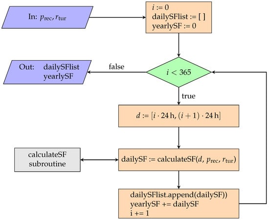
Figure 5. Flow chart diagram for calculating the daily and annual SF for a given year. The input values $p_{\mathrm{rec}}$ and $r_{\mathrm{tur}}$ specify the positions of the receiver and the wind turbine hub, respectively, i iterates over the days of the year, whereas d specifies day i as a time interval. The calculateSF subroutine is provided in Figure 4 as a flow chart diagram and in Algorithm 2 as pseudocode. For simplicity, in the above illustration, we omit the dependency on the specific year and assume it to have 365 days.

7. Correctness

In Section 6.2, we made the following assumptions that influence the correctness of our approach:

(1)

On each day with SF emission, SF only occurs continuously during (i) either a single interval $[t_{\mathrm{SF}-\mathrm{start}},t_{\mathrm{SF}-\mathrm{end}}]$, or (ii) within two distinct intervals at or near the beginning and the end of the day, respectively.

(2)

If the minimization algorithm cannot find a value $t_{\min }\in d$ with ${\mathrm{dist}}_{p_{\mathrm{rec}}}^{+}\left(t_{\min }\right)<0$, then it does not exist.

As the sun position algorithm is very complex, assumption (1) is technically hard to prove while assumption (2) may not even be true. In this section, we explain why it is nonetheless reasonable to make these assumptions.

7.1. Assumption (1): Continuous SF

In this section, we show why it is reasonable to make assumption (1). This assumption can be violated if, within a single day and from the receiver’s perspective, the sun would enter the rotor area, leave it, and reenter it. In Figure 6, this behavior would lead to the sun path entering, exiting, and reentering the region, for which ${\mathrm{dist}}_{p_{\mathrm{rec}}}(\psi ,\theta )<r_{\mathrm{tur}}$. We recall Equation (1):

$$sin\left(\theta \right)=sin\left(\delta \right)sin\left(\lambda \right)+cos\left(\delta \right)cos\left(\lambda \right)cos\left(\omega \right)sin\left(\psi \right)=-{\displaystyle \frac{sin\left(\omega \right)cos\left(\delta \right)}{sin\left(\zeta \right)}}.$$

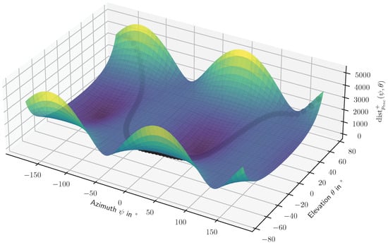
Figure 6. Surface defined by the distance function ${\mathrm{dist}}_{p_{\mathrm{rec}}}(\psi ,\theta )$ for $p_{\mathrm{rec}}={(1000,1000,-100)}^{⊺}$ and $r_{\mathrm{tur}}=40\mathrm{m}$. Each day, the sun follows a path in the azimuth/elevation plane. The azimuth $\psi$ is constantly increasing and ranges from $-180°$ to $180°$. The figure further depicts an exemplary, dotted sun path.

Analyzing the azimuth, we can see that it is constantly increasing (with the exception of being constant in the case of $\lambda =0$). The elevation $\theta$ is just a (horizontally) scaled cos function (assuming $\delta$ and $\lambda$ to be constant within a single day). The elevation function is scaled by a factor between zero and one, thereby preventing large derivatives. As a result, the sun’s movement direction does not change fast enough to enter and exit the SF region twice in all but very extreme cases.

7.2. Assumption (2): Minima

In this section, we show why it is reasonable to make assumption (2). For the numerical minimization algorithm to succeed in finding the minimum, the function ${\mathrm{dist}}_{p_{\mathrm{rec}}}^{+}$ needs to be smooth enough. It is sufficient to look at the distance function ${\mathrm{dist}}_{p_{\mathrm{rec}}}(\psi ,\theta )$, as ${\mathrm{dist}}_{p_{\mathrm{rec}}}^{+}$ does not decrease the function’s smoothness. Recall Equation (7):

$${\mathrm{dist}}_{p_{\mathrm{rec}}}(\psi ,\theta )={∥p^{\ast }∥}_2={∥p_{\mathrm{rec}}-\left({\displaystyle \frac{n_{\mathrm{tur}}·p_{\mathrm{rec}}}{n_{\mathrm{tur}}·n_{\mathrm{sun}}}}\right)·n_{\mathrm{sun}}∥}_2.$$

(14)

As the sun vector $n_{\mathrm{sun}}$ is only relevant for the intersection of the plane defined by the normal vector $n_{\mathrm{tur}}$ and the hub position $p_{\mathrm{tur}}$, we can scale it without changing the result. We define

$$v_{\mathrm{sun}}:=n_{\mathrm{sun}}·{\displaystyle \frac{1}{cos\left(\theta \right)}}=\left(\begin{array}{c}sin\left(\psi \right)\\ cos\left(\psi \right)\\ tan\left(\theta \right)\end{array}\right)$$

and conclude

$$\begin{array}{cc}\hfill {\mathrm{dist}}_{p_{\mathrm{rec}}}(\psi ,\theta )& ={∥p_{\mathrm{rec}}+v_{\mathrm{sun}}·\left(-{\displaystyle \frac{p_{\mathrm{rec}}·n_{\mathrm{tur}}}{v_{\mathrm{sun}}·n_{\mathrm{tur}}}}\right)∥}_2\hfill \\ \hfill & ={∥p_{\mathrm{rec}}-v_{\mathrm{sun}}·\left({\displaystyle \frac{p_{\mathrm{rec},1}·n_{\mathrm{tur},1}+p_{\mathrm{rec},2}·n_{\mathrm{tur},2}}{v_{\mathrm{sun},1}·n_{\mathrm{tur},1}+v_{\mathrm{sun},2}+n_{\mathrm{tur},2}}}\right)∥}_2.\hfill \end{array}$$

Now, $v_{\mathrm{sun},1}=sin\left(\psi \right)=n_{\mathrm{tur},1}$ and $v_{\mathrm{sun},2}=cos\left(\psi \right)=n_{\mathrm{tur},2}$. As ${sin}^2\left(x\right)+{cos}^2\left(x\right)=1$, we obtain

$$\begin{array}{cc}\hfill & {∥p_{\mathrm{rec}}-v_{\mathrm{sun}}·\left({\displaystyle \frac{p_{\mathrm{rec},1}·n_{\mathrm{tur},1}+p_{\mathrm{rec},2}·n_{\mathrm{tur},2}}{v_{\mathrm{sun},1}·n_{\mathrm{tur},1}+v_{\mathrm{sun},2}+n_{\mathrm{tur},2}}}\right)∥}_2\hfill \\ \hfill =& {∥p_{\mathrm{rec}}-v_{\mathrm{sun}}·\left(p_{\mathrm{rec},1}·n_{\mathrm{tur},1}+p_{\mathrm{rec},2}·n_{\mathrm{tur},2}\right)∥}_2\hfill \\ \hfill =& {∥\left(\begin{array}{c}{p}_{\mathrm{rec},1}-v_{\mathrm{sun},1}·\left(p_{\mathrm{rec},1}·n_{\mathrm{tur},1}+p_{\mathrm{rec},2}·n_{\mathrm{tur},2}\right)\\ p_{\mathrm{rec},2}-v_{\mathrm{sun},2}·\left(p_{\mathrm{rec},1}·n_{\mathrm{tur},1}+p_{\mathrm{rec},2}·n_{\mathrm{tur},2}\right)\\ p_{\mathrm{rec},3}-v_{\mathrm{sun},3}·\left(p_{\mathrm{rec},1}·n_{\mathrm{tur},1}+p_{\mathrm{rec},2}·n_{\mathrm{tur},2}\right)\end{array}\right)∥}_2.\hfill \end{array}$$

(15)

Now, the variables $p_{\mathrm{rec},1}$, $p_{\mathrm{rec},2}$ and $p_{\mathrm{rec},3}$ are all real valued. For the other variables, let us take a look at Equation (1) again. We define the following constants:

$$c_1:=sin\left(\delta \right)·sin\left(\lambda \right)c_2:=cos\left(\delta \right)·cos\left(\lambda \right)c_3:=cos\left(\delta \right).$$

Equation (1) can then be rewritten to

$$\begin{array}{cccc}& & \hfill sin\left(\theta \right)& =cos\left(\zeta \right)=c_1+c_2·cos\left(\omega \right)\hfill \\ & \Rightarrow \hfill & \hfill cos\left(\theta \right)& =sin\left(\zeta \right)=\sqrt{1-{cos}^2\left(\zeta \right)}=\sqrt{1-{(c_1+c_2·cos\left(\omega \right))}^2}\hfill \\ & & \hfill sin\left(\psi \right)& =-{\displaystyle \frac{sin\left(\omega \right)·c_3}{sin\left(\zeta \right)}}\hfill \\ & \Rightarrow \hfill & \hfill cos\left(\psi \right)& =\sqrt{1-{sin}^2\left(\psi \right)}=\sqrt{1-{\displaystyle \frac{{sin}^2\left(\omega \right)c_3^2}{{sin}^2\left(\zeta \right)}}}.\hfill \end{array}$$

We can then finally calculate all relevant variables of Equation (15):

$$\begin{array}{cc}\hfill v_{\mathrm{sun},1}& =sin\left(\psi \right)={\displaystyle \frac{-sin\left(\omega \right)·c_3}{\sqrt{1-{(c_1+c_2·cos\left(\omega \right))}^2}}}\hfill \\ \hfill v_{\mathrm{sun},2}& =cos\left(\psi \right)=\sqrt{1-{\displaystyle \frac{{sin}^2\left(\omega \right)·c_3^2}{1-{(c_1+c_2·cos\left(\omega \right))}^2}}}\hfill \\ \hfill v_{\mathrm{sun},3}& =tan\left(\theta \right)={\displaystyle \frac{sin\left(\theta \right)}{cos\left(\theta \right)}}={\displaystyle \frac{c_1+c_2·cos\left(\omega \right)}{\sqrt{1-{(c_1+c_2·cos\left(\omega \right))}^2}}}.\hfill \end{array}$$

Further, $n_{\mathrm{tur},1}=v_{\mathrm{sun},1}$ and $n_{\mathrm{tur},2}=v_{\mathrm{sun},2}$. When inserting the above terms in Equation (15), we can directly calculate ${\mathrm{dist}}_{p_{\mathrm{rec}}}(\psi ,\theta )$. We can see that ${\mathrm{dist}}_{p_{\mathrm{rec}}}(\psi ,\theta )$ is only dependent on the sin and cos terms of the hour angle $\omega$. These are then concatenated using squares, square roots, division, addition, and multiplication. Also, other constants are added and multiplied to terms. As the number of minima in a trigonometric function is bounded for a bounded interval, the number of minima of ${\mathrm{dist}}_{p_{\mathrm{rec}}}(\psi ,\theta )$ is also bounded for a single day. In general, the resulting function does not show any discontinuities or divergence.

Although this does not prove that a minimization algorithm finds the global minimum within a bounded interval, it explains why, in practice, Brent’s minimization does find it.

8. Validation

To illustrate the benefits of our new SF computation method, we implemented and performed a comparative analysis against the traditional discrete approach.

To validate the presented algorithm and show that it provides correct results, an inherent problem is that currently, no algorithm is available to provide the exact SF exposure durations. The only other method available is the discretization method, which inevitably produces a discretization error. To compensate for this error, we have used sampling distances down to 30$\mathrm{s}$.

8.1. Settings

In our case study, we generated shadow flicker maps for a 3000 m × 3000 m area with a single wind turbine placed at the center. Receivers are positioned in a grid using a 50 m step size, resulting in a grid of $61\times 61$ receivers. The turbine used was a Vestas V80, featuring a hub height of 100 m and a rotor diameter of 80 m. For the solar position computations, we employed the geographical coordinates of Aachen, Germany (latitude (50.7753° N), longitude (6.0839° E). For each receiver in the grid, we simulated the annual SF (through iterating over each day of the year). The methods we compared were both written in C and executed on an Apple M1 chip with 8GB of LPDDR4 RAM.

8.2. Results

The results are shown in Table 1 and Figure 7. It is clearly visible that with decreasing sampling size, the result of the discretization method converges toward the result of our new method. This indicates that our new method correctly calculates SF to the precision set for the numerical method. We can further see that while the discrete method becomes more accurate as $\Delta t$ decreases, the computational cost increases significantly. For the same running time, our new method thus achieves a much higher accuracy: The new method is computed with a convergence tolerance of 10⁻³ min in 46.042 s. The discrete method takes about the same time (47.914 s) for a sampling distance $\Delta t$ of 1 $\min$. However, the maximum deviation here is over 10 $\min$. Further, the discrete method can not guarantee any precision, while the convergence tolerance is a parameter for the new method.

Table 1. Evaluation results for the discrete approach using different sampling distances (Section 6.1). Deviations were calculated relative to the continuous method presented in Section 6.2. The running time of the continuous method was 46.042 $\mathrm{s}$ with a convergence tolerance of 10⁻³ $\min$.

$\mathbf{\Delta }\mathit{t}$	Running Time	Avg. Deviation	Mean Deviation	Max. Deviation
[min]	[s]	[%]	[min]	[min]
10.0	8.849	2.5816	11.42	127.47
5.0	12.561	1.0314	4.56	52.21
2.0	26.303	0.3891	1.72	22.30
1.0	47.914	0.2086	0.92	12.31
0.5	93.470	0.1089	0.48	5.45

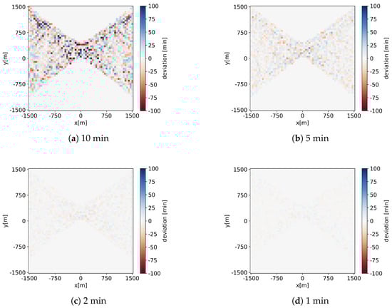
Figure 7. Deviations in annual SF between the discrete algorithm and our new continuous method. For each plot, we have used a different sampling distance.

Looking at Figure 7, we can see that the deviations exhibit a largely stochastic, noise-like pattern across the entire shadowed region. Locations closer to the wind turbine seem to have slightly increased absolute deviations, which could be explained by higher absolute SF values.

Furthermore, we examined the deviation in runtime and precision with different convergence tolerances of the numerical methods. The results of these tests are shown in Table 2. However, decreasing the tolerance did not reduce running time significantly. One explanation of this phenomenon could be the non-linear convergence of Brent’s minimization algorithm and Brent’s root-finding algorithm.

Table 2. Evaluation results for different convergence tolerances of the numerical methods. The first row was used for comparison.

Tolerance	Running Time	Avg. Deviation	Mean Deviation	Max. Deviation
[min]	[s]	[%]	[min]	[min]
10−3	46.042	0.0000	0.0000	0.0000
10−2	43.528	0.0009	0.0041	0.0417
10−1	40.586	0.0121	0.0535	0.9981

9. Conclusions

We presented a novel method to calculate SF durations. In contrast to the existing approach, our method does not use discretization to avoid the discretization error. The core idea of our new method was to model SF using a continuous function. Using numerical minimization and root finding on this function, we were then able to calculate SF with increased accuracy without increasing the running time. Decreasing the accuracy of our algorithm, however, did not lead to significant reductions in running time.

On the practical side, the presented method is modular and could thus be easily integrated into existing wind farm simulation tools such as windPro. On the theoretical side, some feature extensions would be interesting as future work to further improve the accuracy as well as computational efficiency. Regarding accuracy, using statistical weather data may enable to calculate results not only for the worst-case scenario but also for a more realistic one. Regarding efficiency, there is still a lot of potential to further reduce the running time without losing precision. For example, Brent’s minimization algorithm is currently executed until it reaches a certain precision. However, it would be sufficient to stop minimization as soon as a time t with ${\mathrm{dist}}_{p_{\mathrm{rec}}}^{+}\left(t\right)<0$ is found. Furthermore, when simulating each day of a year, we could exploit similarities between successive days to reduce the computational effort. Using these ideas, we expect our new method to become significantly faster than the discretization method (with a sampling distance $\Delta t$ of 1 $\min$), impelling developers to integrate the method into their tools.

In practice, if a wind turbine casts more SF on a receiver than regulations allow, the turbine has to be shut down. Wind farm layout optimization algorithms could use our new method to minimize shutdown times while benefiting from improved accuracy.

In this paper, we only sketched a proof of assumption (1). This was due to the complexity of the underlying sun position algorithm. However, using symbolic simulation with intervals on the sun position algorithm, it may be possible to prove the assumption.

References

- Knopper, L.D.; Ollson, C.A.; McCallum, L.C.; Whitfield Aslund, M.L.; Berger, R.G.; Souweine, K.; McDaniel, M. Wind Turbines and Human Health. Front. Public Health 2014, 2, 63. [Google Scholar] [CrossRef] [PubMed]
- Haac, R.; Darlow, R.; Kaliski, K.; Rand, J.; Hoen, B. In the Shadow of Wind Energy: Predicting Community Exposure and Annoyance to Wind Turbine Shadow Flicker in the United States. Energy Res. Soc. Sci. 2022, 87, 102471. [Google Scholar] [CrossRef]
- EMD International A/S. windPRO User Manual, Chapter 6: Environment; Technical Report; EMD International: Aalborg, Denmark, 2024. [Google Scholar]
- Det Norske Veritas. WindFarmer Calculation Reference. 2023. Available online: https://myworkspace.dnv.com/download/public/renewables/windfarmer/manuals/latest/CalcRef/Introduction/introduction.html (accessed on 6 November 2024).
- Haley, J. Pronghorn Flats Wind Farm Shadow Flicker Analysis Banner and Kimball Counties, NE; Technical Report; EAPC Wind Energy: Norwich, VT, USA, 2020. [Google Scholar]
- SOWIWAS—Energie GmbH. Schattengutachten Ardestorf; Technical Report; SOWIWAS-Energie GmbH: Gevensleben, Germany, 2020. [Google Scholar]
- UL International GmbH. Schattenwurfprognose Elbe Steinlah; Technical Report; UL International GmbH: Oldenburg, Germany, 2020. [Google Scholar]
- Göçmen, T.; van der Laan, P.; Réthoré, P.E.; Diaz, A.P.; Larsen, G.C.; Ott, S. Wind Turbine Wake Models Developed at the Technical University of Denmark: A Review. Renew. Sustain. Energy Rev. 2016, 60, 752–769. [Google Scholar] [CrossRef]
- Shakoor, R.; Hassan, M.Y.; Raheem, A.; Wu, Y.K. Wake Effect Modeling: A Review of Wind Farm Layout Optimization Using Jensen’s Model. Renew. Sustain. Energy Rev. 2016, 58, 1048–1059. [Google Scholar] [CrossRef]
- Azlan, F.; Kurnia, J.C.; Tan, B.T.; Ismadi, M.Z. Review on Optimisation Methods of Wind Farm Array under Three Classical Wind Condition Problems. Renew. Sustain. Energy Rev. 2021, 135, 110047. [Google Scholar] [CrossRef]
- Rediske, G.; Burin, H.P.; Rigo, P.D.; Rosa, C.B.; Michels, L.; Siluk, J.C.M. Wind Power Plant Site Selection: A Systematic Review. Renew. Sustain. Energy Rev. 2021, 148, 111293. [Google Scholar] [CrossRef]
- Meeus, J.H. Astronomical Algorithms; Willmann-Bell, Incorporated: Richmond, VA, USA, 1991. [Google Scholar]
- Reda, I.; Andreas, A. Solar Position Algorithm for Solar Radiation Applications. Solar Energy 2004, 76, 577–589. [Google Scholar] [CrossRef]
- Brent, R.P. Algorithms for Minimization Without Derivatives; Prentice-Hall Series in Automatic Computation; Prentice-Hall, Inc.: Englewood Cliffs, NJ, USA, 1973. [Google Scholar]
- Brent, R.P. An Algorithm with Guaranteed Convergence for Finding a Zero of a Function. Comput. J. 1971, 14, 422–425. [Google Scholar] [CrossRef]
Disclaimer/Publisher’s Note: The statements, opinions and data contained in all publications are solely those of the individual author(s) and contributor(s) and not of MDPI and/or the editor(s). MDPI and/or the editor(s) disclaim responsibility for any injury to people or property resulting from any ideas, methods, instructions or products referred to in the content. |
© 2025 by the authors. Licensee MDPI, Basel, Switzerland. This article is an open access article distributed under the terms and conditions of the Creative Commons Attribution (CC BY) license (https://creativecommons.org/licenses/by/4.0/).