Abstract
With the rapid development and construction of large-scale wind power bases under the “Carbon Peaking and Carbon Neutrality Goals” target, traditional wind energy resource assessment methods typically rely on a limited amount of wind mast data, providing only limited wind resource analysis results. These methods are incapable of capturing the spatiotemporal distribution of wind energy resources throughout the entire base, thus failing to meet the construction requirements of wind power bases. In this study, the mesoscale WRF (The Weather Research and Forecasting Model) was employed for wind resource simulation in a large wind power base. Based on the terrain, meteorological observation data, and boundary conditions, high-resolution wind field simulation results were generated, providing more comprehensive spatiotemporal distribution information within the Ulanqab region’s wind power base. Through the analysis and comparison of measured data and simulation results at different horizontal resolutions, the model was evaluated. Taking the Ulanqab wind power base as an example, the WRF model was used to study the distribution patterns of key parameters, such as annual average wind speed, turbulence intensity, annual average wind power density, and wind direction. The results indicate that a 4 km horizontal resolution can simultaneously ensure the accuracy of wind speed and wind direction simulations, demonstrating good engineering applicability. The analysis of wind resource characteristics in the Ulanqab wind power base based on the mesoscale model provides reliable reference value and data support for its macro- and micro-siting.
1. Introduction
Wind power bases possess advantages not found in traditional wind energy developments [1]. They have high production capacity, economic benefits, and system stability, taking full advantage of geographic features to cluster numerous wind turbines and achieve large-scale wind energy utilization. Such scaled construction significantly enhances wind power generation capacity, increases electricity supply to the grid, and reduces the cost per unit of electricity, yielding better investment returns. The expansion of the base size also improves system stability; by operating multiple turbines in parallel, it can balance the fluctuations in wind energy, ensuring a continuous and stable power supply [2].
Planning for wind power bases requires extensive anemometric tower data, whereas traditional wind resource assessments mainly depend on meteorological stations or anemometric towers. These usually involve few observation sites with inconsistent observation times [3], which are inadequate for the construction needs of wind power bases. Compared to traditional methods, the mesoscale simulation approach WRF (The Weather Research and Forecasting Model) can obtain wind resource parameters for the entire base area, not limited to a few discrete sites. Integrating mesoscale simulation results with actual anemometric tower data enables a more accurate analysis of wind resource distribution characteristics, enhancing the wind resource data within the site [4].
The WRF is a mesoscale meteorological model developed by the U.S. Environmental Prediction Center and Atmospheric Research Center, among others. Its dynamical core uses a fully compressible, non-hydrostatic Eulerian model [5]; the vertical coordinate employs a terrain-following mass coordinate system; the horizontal coordinate uses an Arakawa-C grid; the time integration primarily utilizes a third-order Runge–Kutta scheme; spatial discretization ranges from second to sixth order [6]. Kine Solbakken [7] and others used WRF to assess wind simulations over Norway’s complex terrain, analyzing the impact of atmospheric input data and grid spacing on simulation results. They found that reducing grid spacing from 27 km to 9 km significantly decreases the error in ERA5 simulated wind speeds; however, reducing it further from 3 km to 1 km did not lessen the error. Kunal K.Dayal [8] and others conducted a high-resolution mesoscale wind resource assessment for Fiji, finding that the WRF model’s simulated wind resource parameters closely match measured results, providing reliable wind resource information. Xiangen Liu [9] conducted mesoscale wind field simulations in complex terrain forest areas, indicating that the Noah-MP scheme and YSU scheme are recommended for mesoscale wind simulations in such areas. Talam Enock Kibona [10] used the WRF model to forecast wind energy resources in Tanzania, demonstrating that the WRF model can predict wind characteristics over 72 h, and NCEP data can serve as a wind data source for areas with limited meteorological data.
Building on this research, this paper integrates mesoscale simulation results with actual conditions to better analyze the specific distribution of wind resources at wind power base sites, further refining the wind resource data within the Ulanqab wind power base. However, in practical engineering, an excessive pursuit of high resolution in grid simulation can diminish the impact of disturbances within the mesoscale model, leading to discrepancies between the assessed and actual values of wind resources. Therefore, it is particularly important to consider the relationship between changes in horizontal resolution and the accuracy of mesoscale simulation results. This study aims to conduct a comprehensive examination of the wind resource characteristics in the Ulanqab area using the WRF method, through systematic data collection, meticulous analysis, and precise modeling. It reveals the distribution patterns and trends of wind energy resources in the area, providing data support for the macro- and micro-siting of wind power bases.
2. Overview of the Ulanqab Wind Power Base and Experimental Design
2.1. Basic Information about the Wind Power Base
The terrain of the site is diverse, and Figure 1 shows the elevation map of the simulated area. The central geographic coordinates of the site are (112.57573°, 42.01994°), with a length of approximately 97,170 m and a width of about 56,600 m. The site covers a very wide area, but wind measurement data are only sourced from four anemometric towers within the base. The measured data cover the period from June 2010 to May 2011 (T3961 is missing data for September 2010). Two of the towers, T3943 (112.3373866°, 41.86181172°) and T3961 (112.4067652°, 42.05032825°), are located in relatively complex areas; the other two, T3730 (112.488165°, 41.87955042°) and T3863 (112.4726586°, 41.83487133°), are in relatively flat areas. Their locations are shown in the satellite image in Figure 2. The comparison results of measured data and preliminary simulation data from the four anemometric towers within the base are shown in Appendix A, Table A1. The most significant errors were observed in December; hence, subsequent studies on parameter impacts mainly focus on this month.
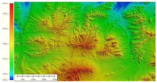
Figure 1.
Topographic elevation map of the Ulanqab wind power base area.
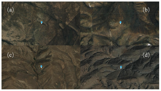
Figure 2.
Satellite images of the wind measurement towers: (a) T3943; (b) T3961; (c) T3730; (d) T3863.
2.2. Selection of Parameterization Schemes
For this study, the WRF model was initialized and driven using data from the NCEP FNL Operational Model Global Tropospheric Analyses [11] (NCEP-FNL), at 6 h intervals. The land use categories in the simulation are based on the USGS (United States Geological Survey) [12] land cover classification, and the projection method used is Lambert. Table 1 summarizes the main physical parameterization schemes used in this WRF model implementation.

Table 1.
Key physical parameterization schemes used in the current WRF model.
2.3. Experimental Design
This study utilizes the WRF model, version 4.3 [22]. Four statistical parameters are employed to perform an independence analysis of the grid: Mean Absolute Error (MAE), Root Mean Square Error (RMSE), Error, and Relative Error, which are used to comprehensively quantify the discrepancies between simulated data and observed data. The Root Mean Square Error (RMSE) represents the differences (referred to as residuals) between predicted values and observed values, indicating the dispersion of the samples; the smaller the RMSE, the better the simulation performance. The Mean Absolute Error (MAE) represents the average of the absolute errors between predicted values and observed values. It is a linear score where all individual differences are weighted equally on the average. MAE directly computes the average of the residuals, whereas RMSE gives more weight to larger differences. The distinctions between these two metrics are attributed to their convergence, uncertainty, and sensitivity to outliers [23].
Mesoscale numerical simulations are conducted using four different horizontal resolutions: 0.5 km, 1 km, 4 km, and 10 km. The nesting scenarios for the four cases are illustrated in Figure 3, with related grid configurations detailed in Table 2, the yellow box in the figure represents the simulation area, and the number 2 represents the domian 2.
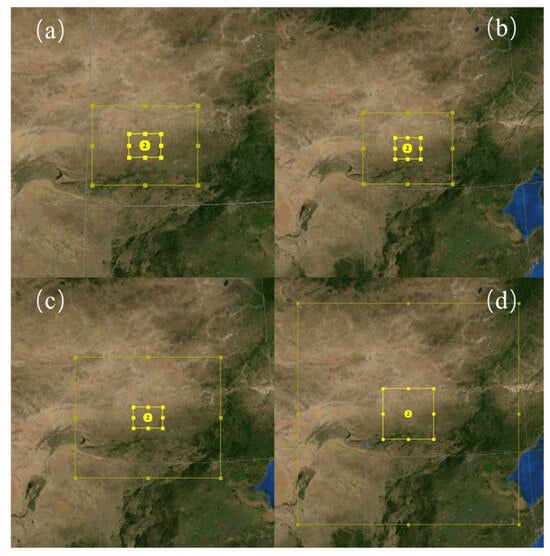
Figure 3.
Nesting schematic for each case: (a) WRF-0.5 km; (b) WRF-1 km; (c) WRF-4 km; (d) WRF-10 km.
Table 2.
Simulation parameter settings for four horizontal resolutions.
The analysis of wind energy resource characteristics at the Ulanqab wind power base primarily focuses on annual average wind speed, time-averaged turbulence intensity, wind power density, and wind direction frequency. Using mesoscale results, the annual average wind speed distribution at various measurement points within the wind power base is calculated to identify the main wind speed intervals. The spatial distribution of turbulence intensity is computed to reveal the impact of terrain and meteorological factors. The wind power density in different areas is calculated to determine the regions richest in wind energy, providing references for wind farm planning. The predominant wind directions are identified to explore the characteristics of wind direction distribution and understand the variations in the wind field.
3. Grid Horizontal Resolution Selection
Four different horizontal resolutions (0.5 km, 1 km, 4 km, 10 km) are used to simulate the region of the large-scale wind power base. The time span is from December 1 to December 31, 2010. To maintain data frequency consistency, the simulation results are chosen as 1 h instantaneous values. Data at a height of 70 m at the grid points corresponding to each anemometer tower are extracted. The wind speed cloud maps are shown in Figure 4.
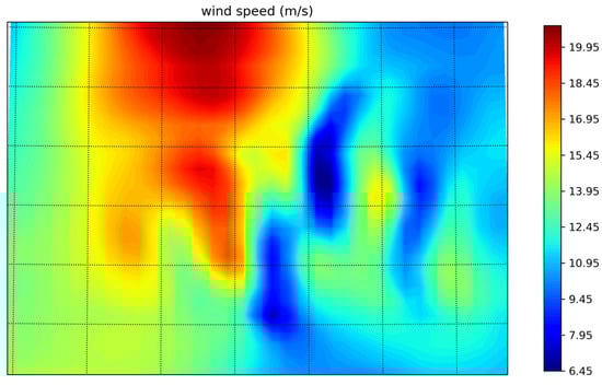
Figure 4.
Mesoscale simulation of wind speed at 70 m (simulates a certain moment in time).
Combining Figure 5a,b and Table 3, it is evident that in the flat terrain at anemometer towers T3730 and T3863, the increasing resolution consistently leads to the wind speed simulation errors trending towards negative values, meaning that the finer the grid, the more likely it is to underestimate the wind speed. For T3730, the wind speed MAE/RMSE at a 4 km resolution are the smallest, at 2.38 m/s and 3.09 m/s, respectively. The wind speed simulation results for T3863 are broadly consistent. For complex terrains, as shown in Figure 5c,d and Table 3, the wind speed simulation errors for towers T3943 and T3961 are also negative. Among them, T3943 at a 4 km grid precision shows the smallest wind speed errors, with MAE/RMSE of 2.50 m/s and 3.11 m/s, respectively. T3961 performs best at WRF-0.5 km and WRF-4 km, though the differences between the two are slight, with WRF-4 km having MAE/RMSE of 3.87 m/s and 4.97 m/s, respectively, compared to the significantly larger errors in the other two cases.
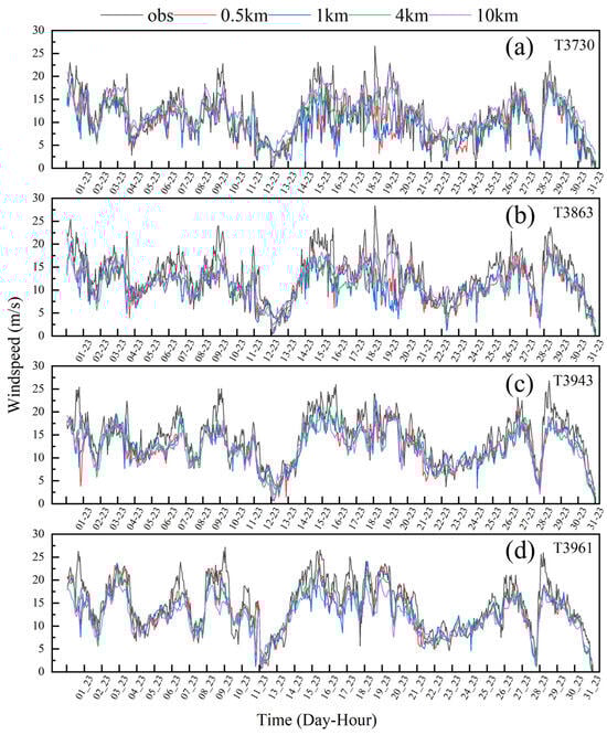
Figure 5.
Comparison of wind speed between WRF results and observed data: (a) T3730; (b) T3863; (c) T3943; (d) T3961.
Table 3.
Wind speed error for grid independence study.
Regarding wind speed errors, among the four anemometer towers, the results corresponding to the WRF-4 km scenario show the smallest errors for two of the towers, and relatively smaller errors for the other two towers in the WRF-4 km scenario. Increasing the horizontal resolution in the WRF model for calculating wind energy resources at large wind power bases does not necessarily optimize simulation effects, a finding echoed in previous studies [24,25]. This indicates that simulation accuracy is also related to terrain complexity and atmospheric stability [4].
The wind direction calculation results for flat terrains are shown in Figure 6a,b. Combined with Table 4, it can be seen that the wind direction simulation errors for anemometer towers T3730 and T3863 are normalized and achieve their minimum values under WRF-4km, at 0.96% and 1.49%, as well as 0.94% and 1.78%, respectively.
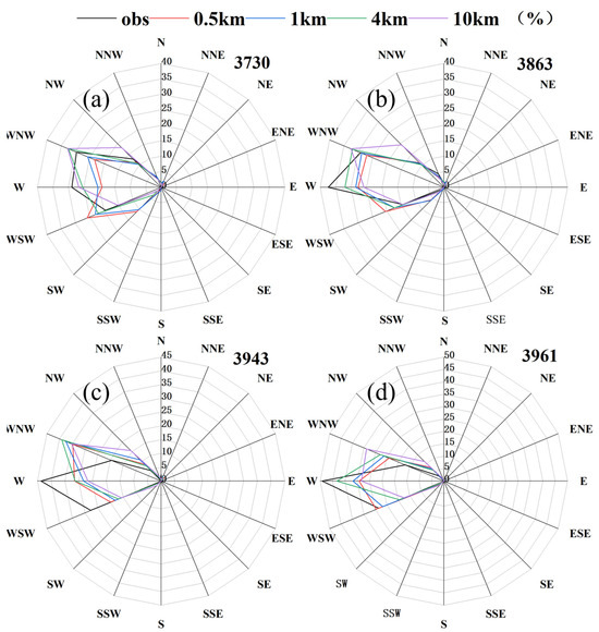
Figure 6.
Comparison of wind direction between WRF results and observed data: (a) T3730; (b) T3863; (c) T3943; (d) T3961.
Table 4.
Wind direction error for grid independence study.
For wind direction simulations in complex terrains, an analysis of Figure 6c,d and Table 4 shows that the wind direction simulation performance of T3943 under WRF-4 km is only second to that under WRF-0.5 km; for T3961, the MAE under WRF-4 km is only 1.99%, and this condition has the smallest RMSE among the four cases.
In summary, conducting mesoscale simulations of wind power bases at a 4 km horizontal resolution can adequately balance the calculation accuracy of both wind speed and direction, while requiring fewer computational resources, making it more suitable for practical engineering applications.
4. Results and Discussion
Based on the study of grid horizontal resolution, the grid horizontal resolution for wind resource calculations is set at 4 km as shown in Figure 7. Within the site, 45 points are selected as the analysis locations for wind resource characteristics, conducting a year-long mesoscale simulation of the Ulanqab wind power base. The main selection criterion involves avoiding the boundaries to prevent the boundary effects from influencing the simulation results; each point represents the wind resource conditions at 70 m height covering a 12 km × 12 km area surrounding it. The parameters included are annual average wind speed, turbulence intensity, annual average wind power density, and various wind directions. The location information for the analysis points of mesoscale wind resource characteristics in the Ulanqab area is shown in Appendix A, Table A2, and the mesoscale simulation wind resource analysis data are shown in Table A3 and Table A4 in Appendix A.
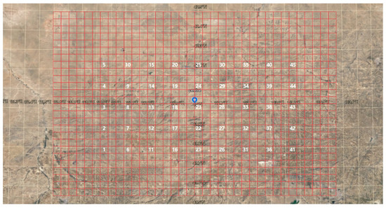
Figure 7.
Illustrative wind map of resource analysis locations in the Ulanqab area; ✩: Site Center.
According to Table A3 and Figure 8, Figure 9 and Figure 10, the annual average wind speed in the Ulanqab wind power base area ranges from 7.327 to 9.131 m/s; turbulence intensity ranges from 0.2877 to 0.3516; and the simulated values for annual average wind power density range from 400 to 727.83 W/m2, with small fluctuations, indicating a relatively stable wind field [26]. In conjunction with related wind resource assessment data, the wind power density level at the base is rated between 5 and 6. The wind speed is at a higher level with minimal fluctuation, showing great potential for wind energy development and suitability for the operation of wind energy equipment.
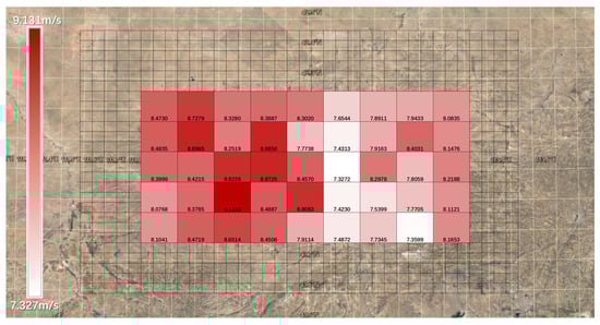
Figure 8.
Illustrative map of annual average wind speed in the Ulanqab wind power base area based on mesoscale simulations.
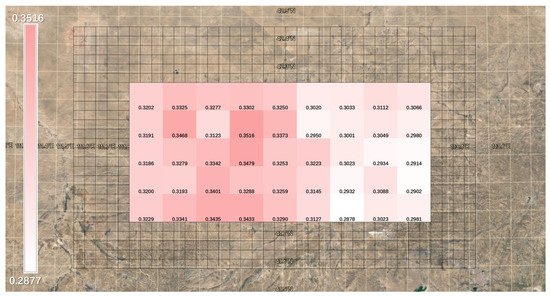
Figure 9.
Illustrative map of turbulence intensity in the Ulanqab wind power base area based on mesoscale simulations.
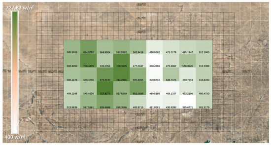
Figure 10.
Illustrative map of annual wind power density in the Ulanqab wind power base area based on mesoscale simulations.
Table A4 provides the distribution of wind direction frequencies at different azimuth angles in the Ulanqab area under mesoscale simulation, with the predominant wind directions being mainly northwest (NNW), west (W), west-southwest (WSW), and north (N). To enhance the utilization rate of wind energy resources, placing wind turbines in the direction of the prevailing winds should be prioritized, and the layout of turbines should consider seasonal changes in wind direction.
In flat terrains, the wind farm can be more easily expanded, maximizing the covered area and enhancing the overall efficiency of wind energy capture. Thus, it is advisable to use an equidistant layout, meaning the distance between each wind turbine is equal. Additionally, it is necessary to optimize the layout of the wind turbines according to the local wind direction patterns, ensuring that turbines capture the maximum wind energy during seasonal wind shifts.
In complex terrains, adjusting the height of wind turbines is often more crucial. By increasing the height of the turbines, the significant impact of terrain obstacles on wind speed can be avoided, reducing the blocking effect between turbines and ensuring that they fully capture wind resources. Flow simulation and wind tunnel experiments can be conducted to understand turbulence, vortices, and wind speed variations within the wind field, determining the optimal layout of the wind turbines.
5. Conclusions
This study used the mesoscale WRF model to investigate the simulation effects of wind energy resources at the Ulanqab wind power base under different horizontal resolutions, specifically analyzing the distribution characteristics of wind resources. The main conclusions are as follows:
- Overly fine horizontal resolution can lead to underestimations of wind speed. Conducting mesoscale simulations of large wind power bases at a 4 km horizontal resolution can adequately balance the calculation accuracy of both wind speed and direction while requiring fewer computational resources, making it more suitable for practical engineering applications.
- In the Ulanqab wind power base area, the annual average wind speed ranges from 7.327 to 9.131 m/s; turbulence intensity ranges from 0.2877 to 0.3516; the measured values for annual average wind power density range from 400 to 727.83 W/m2; and the wind power density level is between 5 and 6. The wind speed is at a high level with minimal fluctuation, showing great potential for wind energy development and suitability for the operation of wind energy equipment.
- In the Ulanqab wind power base, an equidistant layout is recommended for flat terrains to maximize the wind farm’s coverage area. In complex terrains, adjusting the height of wind turbines is more crucial. Increasing the height appropriately can avoid significant impacts of terrain obstacles on wind speed, reduce blocking effects between turbines, and ensure that turbines fully capture wind resources.
Future research could consider using more meteorological data sources to further improve simulation accuracy. For example, incorporating temperature and humidity to gain a more comprehensive understanding of wind resources, refining numerical simulation methods, and enhancing simulation accuracy, especially under complex terrain and variable meteorological conditions. Based on the simulation results and measured data, the planning and layout of wind farms can be optimized to maximize the utilization of available wind resources.
Author Contributions
Methodology, C.X.; Project administration, F.X.; Resources, D.X., W.L. and J.S.; Writing—original draft, Y.W.; Writing—review and editing, Y.L. All authors have read and agreed to the published version of the manuscript.
Funding
This work was supported by the China Power Construction Corporation Research Project, under grant number XBY-ZDKJ-2020-05, the China Power Construction Corporation Research Project under grant number DJ-ZDXM-2020-52, the Fundamental Research Funds for the Central Universities under grant number B240201171, and the National Natural Science Foundation of China under grant number 52106238.
Data Availability Statement
The original contributions presented in the study are included in the article. Further inquiries can be directed to the corresponding authors.
Conflicts of Interest
Authors Dong Xu, Wei Liu and Jing Sun were employed by the company Northwest Engineering Corporation Limited. Author Yuqi Wu was employed by the company China Three Gorges Renewables (Group) Co, Ltd. Eastern construction Management Department of Construction Management Branch. The remaining authors declare that the research was conducted in the absence of any commercial or financial relationships that could be construed as a potential conflict of interest.
Appendix A
Table A1.
Comparison of daily average wind speed MAE, daily average wind speed RMSE, and monthly average wind speed relative error between preliminary simulation data and actual measurements for (a) T3943, (b) T3961, (c) T3730, and (d) T3863.
Table A1.
Comparison of daily average wind speed MAE, daily average wind speed RMSE, and monthly average wind speed relative error between preliminary simulation data and actual measurements for (a) T3943, (b) T3961, (c) T3730, and (d) T3863.
| (a) | |||
| Month | MAE/m·s−1 | RMSE/m·s−1 | Relative Error |
| 2010-6 | 0.972069 | 1.369005 | 12.2970% |
| 2010-7 | 1.495390 | 1.746474 | 18.6485% |
| 2010-8 | 1.308750 | 1.649963 | 14.7526% |
| 2010-9 | 1.647514 | 2.064556 | 23.2959% |
| 2010-10 | 1.562406 | 1.998417 | 18.8081% |
| 2010-11 | 4.313819 | 4.895117 | 35.9706% |
| 2010-12 | 4.551573 | 5.134456 | 32.9202% |
| 2011-1 | 2.889409 | 3.516756 | 24.5647% |
| 2011-2 | 2.308289 | 2.797178 | 28.2564% |
| 2011-3 | 2.670712 | 3.471115 | 25.6852% |
| 2011-4 | 2.007764 | 2.466143 | 20.1443% |
| (b) | |||
| Month | MAE/m·s−1 | RMSE/m·s−1 | Relative Error |
| 2010-6 | 0.975875 | 1.138758 | 3.1128% |
| 2010-7 | 1.103737 | 1.363543 | 8.1692% |
| 2010-8 | 1.273253 | 1.568894 | 12.5209% |
| 2010-10 | 1.306962 | 1.686762 | 8.1646% |
| 2010-11 | 3.432262 | 3.976806 | 26.3689% |
| 2010-12 | 4.380236 | 5.211806 | 30.7107% |
| 2011-1 | 2.423528 | 3.139413 | 23.3169% |
| 2011-2 | 1.929970 | 2.721654 | 18.9256% |
| 2011-3 | 1.544019 | 2.098699 | 9.5772% |
| 2011-4 | 1.554972 | 2.036902 | 8.4051% |
| 2011-5 | 1.758212 | 2.374027 | 11.8054% |
| (c) | |||
| Month | MAE/m·s−1 | RMSE/m·s−1 | Relative Error |
| 2010-6 | 1.149926 | 1.440707 | 13.7023% |
| 2010-7 | 0.896465 | 1.085559 | 7.8385% |
| 2010-8 | 0.811815 | 1.018458 | 8.4693% |
| 2010-9 | 0.901653 | 1.171947 | 6.5620% |
| 2010-10 | 0.736868 | 0.847517 | 6.9692% |
| 2010-11 | 0.859207 | 1.119949 | 5.2778% |
| 2010-12 | 1.414489 | 1.969661 | 7.1658% |
| 2011-1 | 1.055269 | 1.244386 | 3.6111% |
| 2011-2 | 0.867202 | 1.017738 | 6.5577% |
| 2011-3 | 0.865430 | 1.099365 | 2.5069% |
| 2011-4 | 0.739083 | 0.964227 | 0.0835% |
| 2011-5 | 1.005188 | 1.307421 | 1.3272% |
| (d) | |||
| Month | MAE/m·s−1 | RMSE/m·s−1 | Relative Error |
| 2010-6 | 0.828918 | 1.040576 | 0.2558% |
| 2010-7 | 0.96957 | 1.225748 | 4.5730% |
| 2010-8 | 0.830148 | 1.088485 | 6.4043% |
| 2010-9 | 1.047621 | 1.315122 | 6.4676% |
| 2010-10 | 0.996989 | 1.225163 | 8.4948% |
| 2010-11 | 2.320954 | 2.621755 | 20.9120% |
| 2010-12 | 3.075726 | 3.441829 | 23.6107% |
| 2011-1 | 2.244288 | 2.678956 | 19.2064% |
| 2011-2 | 1.355417 | 1.665421 | 12.9593% |
| 2011-3 | 1.850645 | 2.187967 | 17.2335% |
| 2011-4 | 1.17828 | 1.455611 | 11.1761% |
| 2011-5 | 1.463266 | 1.916806 | 12.0390% |
Table A2.
Analysis of the characteristics of the medium-scale wind resources in the Ulanqab region.
Table A2.
Analysis of the characteristics of the medium-scale wind resources in the Ulanqab region.
| Point Number | Longitude/° | Latitude/° |
|---|---|---|
| 1 | 112.0026 | 41.77696 |
| 2 | 112.0015 | 41.88849 |
| 3 | 112.0004 | 42.00002 |
| 4 | 112.0009 | 42.11265 |
| 5 | 111.9982 | 42.22314 |
| 6 | 111.9982 | 42.22314 |
| 7 | 111.9982 | 42.22314 |
| 8 | 111.9982 | 42.22314 |
| 9 | 112.1498 | 42.11224 |
| 10 | 112.149 | 42.22381 |
| 11 | 112.3017 | 41.77807 |
| 12 | 112.3012 | 41.88959 |
| 13 | 112.3007 | 42.00114 |
| 14 | 112.3002 | 42.11269 |
| 15 | 112.2997 | 42.22426 |
| 16 | 112.4513 | 41.77831 |
| 17 | 112.4511 | 41.88984 |
| 18 | 112.4509 | 42.00139 |
| 19 | 112.4506 | 42.11293 |
| 20 | 112.4504 | 42.22451 |
| 21 | 112.6009 | 41.77834 |
| 22 | 112.601 | 41.88987 |
| 23 | 112.601 | 42.00143 |
| 24 | 112.6011 | 42.11298 |
| 25 | 112.6011 | 42.22455 |
| 26 | 112.7505 | 41.77818 |
| 27 | 112.7509 | 41.88971 |
| 28 | 112.7512 | 42.00124 |
| 29 | 112.7515 | 42.1128 |
| 30 | 112.7518 | 42.22437 |
| 31 | 112.9001 | 41.77779 |
| 32 | 112.9007 | 41.88932 |
| 33 | 112.9013 | 42.00087 |
| 34 | 112.9019 | 42.11242 |
| 35 | 112.9025 | 42.22397 |
| 36 | 113.0497 | 41.77721 |
| 37 | 113.0506 | 41.88873 |
| 38 | 113.0515 | 42.00027 |
| 39 | 113.0524 | 42.11182 |
| 40 | 113.0533 | 42.22339 |
| 41 | 113.1993 | 41.7764 |
| 42 | 113.2004 | 41.88792 |
| 43 | 113.2016 | 41.99947 |
| 44 | 113.2028 | 42.11102 |
| 45 | 113.204 | 42.22258 |
Table A3.
Mid-scale wind resource table for Ulanqab region (annual average wind speed, turbulence intensity, annual average wind power density).
Table A3.
Mid-scale wind resource table for Ulanqab region (annual average wind speed, turbulence intensity, annual average wind power density).
| Point Numbe | Annual Average Wind Speed/m·s−1 | Turbulence Intensity | Annual Average Wind Power Density/W·m−2 |
|---|---|---|---|
| 1 | 8.1041101 | 0.3229286 | 513.6839459 |
| 2 | 8.0767585 | 0.3199952 | 499.2297909 |
| 3 | 8.3998524 | 0.3186319 | 560.1277942 |
| 4 | 8.483543 | 0.319104 | 582.9049902 |
| 5 | 8.472975 | 0.320163 | 585.9553334 |
| 6 | 8.471918 | 0.334064 | 587.5160964 |
| 7 | 8.378492 | 0.319339 | 548.9150254 |
| 8 | 8.421547 | 0.327882 | 579.4736091 |
| 9 | 8.896453 | 0.346759 | 700.437858 |
| 10 | 8.727921 | 0.33253 | 654.3782222 |
| 11 | 8.651424 | 0.343526 | 636.4947688 |
| 12 | 9.131844 | 0.340107 | 727.8269875 |
| 13 | 8.822581 | 0.334211 | 675.0139863 |
| 14 | 8.251927 | 0.312326 | 536.0354253 |
| 15 | 8.327987 | 0.32769 | 564.9023567 |
| 16 | 8.450591 | 0.343339 | 595.3066167 |
| 17 | 8.488663 | 0.328766 | 597.6369231 |
| 18 | 8.872523 | 0.34792 | 713.2900586 |
| 19 | 8.88502 | 0.351634 | 708.592505 |
| 20 | 8.388699 | 0.330233 | 592.538197 |
| 21 | 7.911385 | 0.328983 | 483.8715135 |
| 22 | 8.80834 | 0.325949 | 651.0879919 |
| 23 | 8.457009 | 0.325289 | 605.6354951 |
| 24 | 7.773824 | 0.337327 | 477.0047165 |
| 25 | 8.302027 | 0.325018 | 562.9418033 |
| 26 | 7.487173 | 0.31269 | 411.9261171 |
| 27 | 7.422982 | 0.314516 | 410.5165645 |
| 28 | 7.327178 | 0.322299 | 400.671643 |
| 29 | 7.43128 | 0.295024 | 390.4567518 |
| 30 | 7.654353 | 0.301992 | 438.9282381 |
| 31 | 7.359871 | 0.302284 | 385.6770955 |
| 32 | 7.770468 | 0.308827 | 453.2196023 |
| 33 | 7.805937 | 0.293372 | 449.7654077 |
| 34 | 8.403074 | 0.304882 | 556.9544909 |
| 35 | 7.943344 | 0.31121 | 495.1347244 |
| 36 | 7.734493 | 0.28777 | 430.8280079 |
| 37 | 7.539879 | 0.293231 | 408.1337379 |
| 38 | 8.297772 | 0.302325 | 539.747534 |
| 39 | 7.916337 | 0.300147 | 475.6981808 |
| 40 | 7.891123 | 0.303338 | 471.0177723 |
| 41 | 8.165283 | 0.298124 | 501.5179189 |
| 42 | 8.112145 | 0.290225 | 490.4749924 |
| 43 | 8.218756 | 0.291404 | 515.6343216 |
| 44 | 8.147643 | 0.298013 | 513.238947 |
| 45 | 8.083455 | 0.306622 | 512.1800006 |
Table A4.
Mid-scale wind resource table for Ulanqab region (wind direction).
Table A4.
Mid-scale wind resource table for Ulanqab region (wind direction).
| Number | Azimuth Angle Frequency | N | NNE | NE | ENE |
|---|---|---|---|---|---|
| 1 | 0.14 | 0.179 | 0.098 | 0.047 | |
| 2 | 0.139 | 0.191 | 0.1 | 0.045 | |
| 3 | 0.165 | 0.188 | 0.089 | 0.042 | |
| 4 | 0.192 | 0.17 | 0.078 | 0.039 | |
| 5 | 0.209 | 0.148 | 0.072 | 0.042 | |
| 6 | 0.17 | 0.204 | 0.099 | 0.044 | |
| 7 | 0.158 | 0.198 | 0.103 | 0.048 | |
| 8 | 0.169 | 0.158 | 0.075 | 0.041 | |
| 9 | 0.206 | 0.175 | 0.075 | 0.044 | |
| 10 | 0.223 | 0.151 | 0.079 | 0.046 | |
| 11 | 0.181 | 0.22 | 0.091 | 0.043 | |
| 12 | 0.176 | 0.208 | 0.108 | 0.053 | |
| 13 | 0.197 | 0.181 | 0.085 | 0.051 | |
| 14 | 0.171 | 0.169 | 0.083 | 0.053 | |
| 15 | 0.197 | 0.148 | 0.087 | 0.042 | |
| 16 | 0.188 | 0.221 | 0.091 | 0.048 | |
| 17 | 0.168 | 0.178 | 0.106 | 0.057 | |
| 18 | 0.202 | 0.189 | 0.088 | 0.054 | |
| 19 | 0.201 | 0.183 | 0.097 | 0.052 | |
| 20 | 0.204 | 0.164 | 0.088 | 0.047 | |
| 21 | 0.186 | 0.194 | 0.104 | 0.055 | |
| 22 | 0.156 | 0.209 | 0.12 | 0.062 | |
| 23 | 0.162 | 0.192 | 0.107 | 0.062 | |
| 24 | 0.165 | 0.166 | 0.104 | 0.059 | |
| 25 | 0.183 | 0.191 | 0.086 | 0.059 | |
| 26 | 0.164 | 0.165 | 0.11 | 0.068 | |
| 27 | 0.124 | 0.156 | 0.141 | 0.086 | |
| 28 | 0.112 | 0.202 | 0.136 | 0.069 | |
| 29 | 0.143 | 0.174 | 0.106 | 0.062 | |
| 30 | 0.155 | 0.169 | 0.082 | 0.056 | |
| 31 | 0.134 | 0.154 | 0.136 | 0.083 | |
| 32 | 0.103 | 0.171 | 0.171 | 0.071 | |
| 33 | 0.114 | 0.214 | 0.116 | 0.059 | |
| 34 | 0.157 | 0.177 | 0.102 | 0.057 | |
| 35 | 0.166 | 0.177 | 0.09 | 0.053 | |
| 36 | 0.121 | 0.15 | 0.165 | 0.067 | |
| 37 | 0.113 | 0.181 | 0.127 | 0.061 | |
| 38 | 0.126 | 0.188 | 0.118 | 0.068 | |
| 39 | 0.137 | 0.171 | 0.119 | 0.062 | |
| 40 | 0.161 | 0.177 | 0.09 | 0.053 | |
| 41 | 0.117 | 0.174 | 0.154 | 0.071 | |
| 42 | 0.118 | 0.173 | 0.135 | 0.07 | |
| 43 | 0.116 | 0.177 | 0.135 | 0.064 | |
| 44 | 0.14 | 0.184 | 0.106 | 0.057 | |
| 45 | 0.159 | 0.174 | 0.092 | 0.058 | |
| Number | Azimuth Angle Frequency | N | NNE | NE | ENE |
| 1 | 0.029 | 0.026 | 0.024 | 0.021 | |
| 2 | 0.03 | 0.026 | 0.027 | 0.022 | |
| 3 | 0.032 | 0.024 | 0.024 | 0.028 | |
| 4 | 0.035 | 0.024 | 0.024 | 0.024 | |
| 5 | 0.032 | 0.022 | 0.026 | 0.028 | |
| 6 | 0.032 | 0.025 | 0.021 | 0.024 | |
| 7 | 0.035 | 0.03 | 0.026 | 0.021 | |
| 8 | 0.035 | 0.031 | 0.027 | 0.025 | |
| 9 | 0.035 | 0.027 | 0.026 | 0.025 | |
| 10 | 0.034 | 0.026 | 0.028 | 0.029 | |
| 11 | 0.033 | 0.028 | 0.031 | 0.022 | |
| 12 | 0.039 | 0.028 | 0.028 | 0.02 | |
| 13 | 0.032 | 0.024 | 0.025 | 0.024 | |
| 14 | 0.036 | 0.025 | 0.025 | 0.021 | |
| 15 | 0.035 | 0.025 | 0.027 | 0.027 | |
| 16 | 0.043 | 0.037 | 0.021 | 0.02 | |
| 17 | 0.044 | 0.043 | 0.025 | 0.014 | |
| 18 | 0.038 | 0.032 | 0.028 | 0.021 | |
| 19 | 0.036 | 0.031 | 0.028 | 0.02 | |
| 20 | 0.034 | 0.027 | 0.031 | 0.024 | |
| 21 | 0.047 | 0.038 | 0.025 | 0.021 | |
| 22 | 0.047 | 0.035 | 0.025 | 0.018 | |
| 23 | 0.042 | 0.034 | 0.022 | 0.016 | |
| 24 | 0.042 | 0.033 | 0.027 | 0.018 | |
| 25 | 0.04 | 0.033 | 0.029 | 0.023 | |
| 26 | 0.06 | 0.036 | 0.021 | 0.014 | |
| 27 | 0.054 | 0.033 | 0.02 | 0.012 | |
| 28 | 0.041 | 0.029 | 0.022 | 0.015 | |
| 29 | 0.042 | 0.037 | 0.029 | 0.019 | |
| 30 | 0.04 | 0.033 | 0.032 | 0.022 | |
| 31 | 0.041 | 0.028 | 0.024 | 0.015 | |
| 32 | 0.041 | 0.029 | 0.026 | 0.016 | |
| 33 | 0.042 | 0.034 | 0.029 | 0.021 | |
| 34 | 0.044 | 0.038 | 0.029 | 0.022 | |
| 35 | 0.041 | 0.034 | 0.027 | 0.022 | |
| 36 | 0.047 | 0.029 | 0.023 | 0.015 | |
| 37 | 0.049 | 0.033 | 0.026 | 0.015 | |
| 38 | 0.052 | 0.031 | 0.025 | 0.014 | |
| 39 | 0.049 | 0.031 | 0.027 | 0.017 | |
| 40 | 0.043 | 0.035 | 0.028 | 0.025 | |
| 41 | 0.051 | 0.031 | 0.022 | 0.016 | |
| 42 | 0.052 | 0.03 | 0.022 | 0.015 | |
| 43 | 0.051 | 0.03 | 0.025 | 0.014 | |
| 44 | 0.049 | 0.031 | 0.028 | 0.017 | |
| 45 | 0.046 | 0.032 | 0.027 | 0.023 | |
| Number | Azimuth Angle Frequency | N | NNE | NE | ENE |
| 1 | 0.021 | 0.018 | 0.018 | 0.017 | |
| 2 | 0.015 | 0.018 | 0.025 | 0.021 | |
| 3 | 0.022 | 0.015 | 0.016 | 0.019 | |
| 4 | 0.024 | 0.021 | 0.019 | 0.016 | |
| 5 | 0.024 | 0.021 | 0.02 | 0.017 | |
| 6 | 0.021 | 0.018 | 0.023 | 0.019 | |
| 7 | 0.015 | 0.017 | 0.025 | 0.022 | |
| 8 | 0.018 | 0.015 | 0.016 | 0.02 | |
| 9 | 0.019 | 0.022 | 0.018 | 0.019 | |
| 10 | 0.024 | 0.018 | 0.021 | 0.022 | |
| 11 | 0.016 | 0.018 | 0.021 | 0.021 | |
| 12 | 0.014 | 0.014 | 0.02 | 0.023 | |
| 13 | 0.019 | 0.017 | 0.021 | 0.022 | |
| 14 | 0.02 | 0.024 | 0.022 | 0.021 | |
| 15 | 0.02 | 0.017 | 0.021 | 0.023 | |
| 16 | 0.013 | 0.015 | 0.02 | 0.023 | |
| 17 | 0.011 | 0.011 | 0.018 | 0.026 | |
| 18 | 0.014 | 0.015 | 0.016 | 0.023 | |
| 19 | 0.017 | 0.019 | 0.024 | 0.029 | |
| 20 | 0.017 | 0.015 | 0.022 | 0.034 | |
| 21 | 0.012 | 0.015 | 0.022 | 0.026 | |
| 22 | 0.011 | 0.015 | 0.021 | 0.03 | |
| 23 | 0.013 | 0.016 | 0.024 | 0.034 | |
| 24 | 0.011 | 0.015 | 0.023 | 0.05 | |
| 25 | 0.017 | 0.014 | 0.014 | 0.041 | |
| 26 | 0.009 | 0.015 | 0.024 | 0.035 | |
| 27 | 0.013 | 0.012 | 0.022 | 0.042 | |
| 28 | 0.011 | 0.013 | 0.022 | 0.074 | |
| 29 | 0.011 | 0.013 | 0.016 | 0.066 | |
| 30 | 0.019 | 0.015 | 0.011 | 0.028 | |
| 31 | 0.009 | 0.017 | 0.029 | 0.046 | |
| 32 | 0.013 | 0.016 | 0.024 | 0.047 | |
| 33 | 0.011 | 0.016 | 0.016 | 0.05 | |
| 34 | 0.012 | 0.016 | 0.014 | 0.03 | |
| 35 | 0.017 | 0.017 | 0.019 | 0.033 | |
| 36 | 0.01 | 0.015 | 0.028 | 0.055 | |
| 37 | 0.011 | 0.016 | 0.021 | 0.05 | |
| 38 | 0.01 | 0.016 | 0.017 | 0.041 | |
| 39 | 0.011 | 0.015 | 0.016 | 0.036 | |
| 40 | 0.016 | 0.014 | 0.013 | 0.034 | |
| 41 | 0.01 | 0.016 | 0.025 | 0.054 | |
| 42 | 0.011 | 0.014 | 0.021 | 0.053 | |
| 43 | 0.01 | 0.016 | 0.015 | 0.045 | |
| 44 | 0.015 | 0.016 | 0.014 | 0.035 | |
| 45 | 0.014 | 0.018 | 0.015 | 0.029 | |
| Number | Azimuth Angle Frequency | N | NNE | NE | ENE |
| 1 | 0.031 | 0.078 | 0.121 | 0.132 | |
| 2 | 0.027 | 0.071 | 0.119 | 0.123 | |
| 3 | 0.031 | 0.074 | 0.114 | 0.116 | |
| 4 | 0.028 | 0.073 | 0.109 | 0.124 | |
| 5 | 0.024 | 0.067 | 0.106 | 0.141 | |
| 6 | 0.026 | 0.053 | 0.103 | 0.121 | |
| 7 | 0.027 | 0.046 | 0.109 | 0.12 | |
| 8 | 0.03 | 0.061 | 0.131 | 0.148 | |
| 9 | 0.024 | 0.043 | 0.113 | 0.13 | |
| 10 | 0.022 | 0.041 | 0.101 | 0.134 | |
| 11 | 0.029 | 0.043 | 0.093 | 0.112 | |
| 12 | 0.027 | 0.037 | 0.08 | 0.126 | |
| 13 | 0.028 | 0.04 | 0.099 | 0.136 | |
| 14 | 0.025 | 0.044 | 0.12 | 0.14 | |
| 15 | 0.023 | 0.05 | 0.124 | 0.132 | |
| 16 | 0.029 | 0.045 | 0.083 | 0.103 | |
| 17 | 0.034 | 0.044 | 0.085 | 0.136 | |
| 18 | 0.039 | 0.043 | 0.076 | 0.12 | |
| 19 | 0.032 | 0.031 | 0.066 | 0.133 | |
| 20 | 0.036 | 0.032 | 0.09 | 0.134 | |
| 21 | 0.027 | 0.048 | 0.087 | 0.094 | |
| 22 | 0.028 | 0.039 | 0.076 | 0.108 | |
| 23 | 0.03 | 0.045 | 0.088 | 0.114 | |
| 24 | 0.037 | 0.053 | 0.079 | 0.12 | |
| 25 | 0.056 | 0.047 | 0.061 | 0.107 | |
| 26 | 0.039 | 0.056 | 0.102 | 0.082 | |
| 27 | 0.056 | 0.058 | 0.082 | 0.088 | |
| 28 | 0.07 | 0.046 | 0.058 | 0.078 | |
| 29 | 0.071 | 0.047 | 0.067 | 0.097 | |
| 30 | 0.066 | 0.076 | 0.091 | 0.104 | |
| 31 | 0.047 | 0.058 | 0.101 | 0.08 | |
| 32 | 0.051 | 0.054 | 0.084 | 0.082 | |
| 33 | 0.06 | 0.07 | 0.075 | 0.074 | |
| 34 | 0.056 | 0.074 | 0.072 | 0.1 | |
| 35 | 0.049 | 0.071 | 0.08 | 0.103 | |
| 36 | 0.054 | 0.05 | 0.082 | 0.09 | |
| 37 | 0.061 | 0.066 | 0.089 | 0.081 | |
| 38 | 0.062 | 0.064 | 0.087 | 0.08 | |
| 39 | 0.067 | 0.071 | 0.088 | 0.084 | |
| 40 | 0.074 | 0.072 | 0.075 | 0.092 | |
| 41 | 0.061 | 0.047 | 0.064 | 0.087 | |
| 42 | 0.065 | 0.054 | 0.074 | 0.092 | |
| 43 | 0.067 | 0.064 | 0.088 | 0.082 | |
| 44 | 0.068 | 0.073 | 0.083 | 0.084 | |
| 45 | 0.067 | 0.072 | 0.081 | 0.093 | |
References
- Wang, Q.; Luo, K.; Wu, C.L.; Zhu, Z.F.; Fan, J.R. Mesoscale simulations of a real onshore wind power base in complex terrain: Wind farm wake behavior and power production. Energy 2022, 241, 122873. [Google Scholar] [CrossRef]
- Prósper, M.A.; Otero-Casal, C.; Fernández, F.C.; Miguez-Macho, G. Wind power forecasting for a real onshore wind farm on complex terrain using WRF high resolution simulations. Renew. Energy 2019, 135, 674–686. [Google Scholar] [CrossRef]
- Sun, X.J.; Huang, D.G. An Explosive Growth of Wind Power in China. Int. J. Green Energy 2014, 11, 849–860. [Google Scholar] [CrossRef]
- Yuan, R.; Ji, W.; Luo, K.; Wang, J.; Zhang, S.; Wang, Q.; Fan, J.; Ni, M.; Cen, K. Coupled wind farm parameterization with a mesoscale model for simulations of an onshore wind farm. Appl. Energy 2017, 206, 113–125. [Google Scholar] [CrossRef]
- Laprise, R. The Euler equations of motion with hydrostatic pressure as an independent variable. Mon. Weather Rev. 1992, 120, 197–207. [Google Scholar] [CrossRef]
- Fang, F.; Xiaoning, Z.; Guishan, Y.; Yang, H.; Yuchen, H. Assessment of the Impact of Wake Interference Within Onshore and Offshore Wind Farms Based on Mesoscale Meteorological Model Analysis. Proc. CSEE 2022, 42, 4848–4859. (In Chinese) [Google Scholar] [CrossRef]
- Solbakken, K.; Birkelund, Y.; Samuelsen, E.M. Evaluation of surface wind using WRF in complex terrain: Atmospheric input data and grid spacing. Environ. Modell Softw. 2021, 145, 105182. [Google Scholar] [CrossRef]
- Dayal, K.K.; Bellon, G.; Cater, J.E.; Kingan, M.J.; Sharma, R.N. High-resolution mesoscale wind-resource assessment of Fiji using the Weather Research and Forecasting (WRF) model. Energy 2021, 232, 121047. [Google Scholar] [CrossRef]
- Liu, X.; Cao, J.; Xin, D. Wind field numerical simulation in forested regions of complex terrain: A mesoscale study using WRF. J. Wind Eng. Ind. Aerodyn. 2022, 222, 104915. [Google Scholar] [CrossRef]
- Kibona, T.E. Application of WRF mesoscale model for prediction of wind energy resources in Tanzania. Sci. Afr. 2020, 7, e00302. [Google Scholar] [CrossRef]
- National Centers for Environmental Prediction; National Weather Service; NOAA; U.S. Department of Commerce. NCEP FNL Operational Model Global Tropospheric Analyses, Continuing from July 1999; National Center for Atmospheric Research, Computational and Information Systems Laboratory: Boulder, CO, USA, 2000. [CrossRef]
- López-Vázquez, C.; Ariza-López, F.J. Global Digital Elevation Model Comparison Criteria: An Evident Need to Consider Their Application. ISPRS Int. J. Geo-Inf. 2023, 12, 337. [Google Scholar] [CrossRef]
- Thompson, G.; Field, P.R.; Rasmussen, R.M.; Hall, W.D. Explicit Forecasts of Winter Precipitation Using an Improved Bulk Microphysics Scheme. Part II: Implementation of a New Snow Parameterization. Mon. Weather Rev. 2008, 136, 5095–5115. [Google Scholar] [CrossRef]
- Hong, S.; Lim, J.J. The WRF single-moment 6-class microphysics scheme (WSM6). Asia-Pac. J. Atmos. Sci. 2006, 42, 129–151. [Google Scholar]
- Hong, S.-Y.; Lim, J.-O.J. The WRF single–moment 6–class microphysics scheme (WSM6). J. Korean Meteor. Soc. 2017, 42, 129–151. [Google Scholar] [CrossRef]
- Dudhia, J. Numerical study of convection observed during the winter monsoon experiment using a mesoscale two-dimensional model. J. Atmos. Sci. 1989, 46, 3077–3107. [Google Scholar] [CrossRef]
- Mlawer, E.J.; Taubman, S.J.; Brown, P.D.; Iacono, M.J.; Clough, S.A. Radiative transfer for inhomogeneous atmospheres: RRTM, a validated correlated-k model for the longwave. J. Geophys. Res. Atmos. 1997, 102, 16663–16682. [Google Scholar] [CrossRef]
- Paulson, C.A. The mathematical representation of wind speed and temperature profiles in the unstable atmospheric surface layer. J. Appl. Meteorol. Clim. 1970, 9, 857–861. [Google Scholar] [CrossRef]
- Chen, F.; Dudhia, J. Coupling an advanced land surface–hydrology model with the Penn State–NCAR MM5 modeling system. Part I: Model implementation and sensitivity. Mon. Weather Rev. 2001, 129, 569–585. [Google Scholar] [CrossRef]
- Hong, S.; Noh, Y.; Dudhia, J. A new vertical diffusion package with an explicit treatment of entrainment processes. Mon. Weather Rev. 2006, 134, 2318–2341. [Google Scholar] [CrossRef]
- Grell, G.A.; Freitas, S.R. A scale and aerosol aware stochastic convective parameterization for weather and air quality modeling. Atmos. Chem. Phys. 2014, 14, 5233–5250. [Google Scholar] [CrossRef]
- Skamarock, W.C.; Klemp, J.B.; Dudhia, J.; Gill, D.O.; Liu, Z.; Berner, J.; Wang, W.; Powers, J.G.; Duda, M.G.; Barker, D.; et al. A Description of the Advanced Research WRF Model Version 4.3. 2021, No. NCAR/TN-556+STR. Available online: https://opensky.ucar.edu/islandora/object/opensky:2898 (accessed on 14 July 2024).
- Schneider, P.; Xhafa, F. Chapter 3—Anomaly detection: Concepts and methods. In Anomaly Detection and Complex Event Processing over IoT Data Streams; Academic Press: Cambridge, MA, USA, 2022; pp. 49–66. [Google Scholar] [CrossRef]
- Marjanovic, N.; Wharton, S.; Chow, F.K. Investigation of model parameters for high-resolution wind energy forecasting: Case studies over simple and complex terrain. J. Wind Eng. Ind. Aerodyn. 2014, 134, 10–24. [Google Scholar] [CrossRef]
- Giannakopoulou, E.; Nhili, R. WRF model methodology for offshore wind energy applications. Adv. Meteorol. 2014, 2014, 319819. [Google Scholar] [CrossRef]
- Yang, J.; Zhang, C.; Sun, Q.Y.; Wang, G. Review of wind farm site selection. Acta Energiae Solaris Sin. 2012, 33, 136–144. [Google Scholar]
Disclaimer/Publisher’s Note: The statements, opinions and data contained in all publications are solely those of the individual author(s) and contributor(s) and not of MDPI and/or the editor(s). MDPI and/or the editor(s) disclaim responsibility for any injury to people or property resulting from any ideas, methods, instructions or products referred to in the content. |
© 2024 by the authors. Licensee MDPI, Basel, Switzerland. This article is an open access article distributed under the terms and conditions of the Creative Commons Attribution (CC BY) license (https://creativecommons.org/licenses/by/4.0/).