Robust Control Based on Observed States Designed by Means of Linear Matrix Inequalities for Grid-Connected Converters

Abstract

This paper provides a procedure to design robust controllers based on observed states applied to three-phase inverters with LCL filters connected to a grid with uncertain and possibly time-varying impedances, which can arise in renewable energy systems and microgrid applications. Linear matrix inequalities are used to rapidly compute, off-line, based only on the choice of two scalar parameters for pole location, sets of gains for the controller and the observer, and also to provide a theoretical certificate of the closed-loop stability, including a limit for the rate of variations of the grid impedances. The proposed design procedure allows the easy implementation of robust state feedback controllers with a reduced number of sensors, ensuring good performance for different sets of grid impedances. Additionally, larger regions of guaranteed stability are provided by the proposed procedure, when compared with a similar condition from the literature. The control law using the observed states can ensure grid currents with low harmonic content, complying with the IEEE 1547 Standard requirements, with negligible loss of performance concerning the feedback of the measured state variables. Three optimal state feedback controllers from the literature are reproduced here and successfully implemented using the observed state variables based on the proposed procedure. In all cases, the viability of the proposal was confirmed by simulations and experimental results.

1. Introduction

The demand for electrical energy is growing throughout the world [1,2], since energy is fundamental for industrial, agricultural, commercial and domestic activities, among others. However, a great part of the generation of energy is still carbon-dependent [3], mainly based on fossil fuel, such as coal, gas, and oil [4]. This carbon-dependent generation impacts negatively on the environmental balance [5]. According to the International Renewable Energy Agency (IRENA), it is necessary to replace energy sources from fossil hydrocarbon fuels to clean energy sources until 2040–2050 [6]. Thus, many countries are facing challenges to develop policies and strategies for expanding sustainable energy systems [7]. Renewable Energy Systems (RES), such as solar and wind, for example, are fundamental for expanding the energy matrices [8,9,10]. A very important issue for improving these sustainable energy systems is improving the energy quality, which can be achieved, for instance, by reducing the Total Harmonic Distortion (THD) in the grid-injected currents for RES that use DC-AC converters [11]. Voltage source inverters are a key part to control the power flow between the primary sources and the mains [12]. Suitable synchronization and current controllers can ensure that the currents injected into the grid comply with limits for harmonic distortion. In order to reduce harmonic content, LCL filters are widely used as the output stage of the inverters [3,4,13,14,15]. However, these filters present a resonance that usually demands damping, which is more challenging considering the need to ensure stability and performance for systems subject to uncertain and possibly time-variant parameters, as is usually the case of the impedance at the point of common coupling in distributed generation systems and microgrid applications [5,16]. In this context, an alternative for active damping is the robust state feedback control strategy, which is able to attenuate the resonance peak of the filter for an entire range of grid impedances [6,17].

A well-established tool in control theory to design robust state feedback controllers systematically and efficiently are the linear matrix inequalities (LMIs) [18]. If the design problem can be written as an LMI problem, it has the guarantee to be solved in polynomial time by specialized algorithms, with global convergence [19]. Considering grid-connected converters with LCL filters, LMIs have been successfully applied for robust control design based on full-state feedback, for instance, in [20,21,22,23]. These works show guidelines on the use of suboptimal controllers, viable for practical applications, allowing good tradeoffs between robustness and performance. On the other hand, although full-state feedback techniques can ensure stability and suitable results, they usually rely on the measurement of all LCL filter state variables. To avoid that, state observers are an important alternative, allowing the implementation of control strategies with a reduced number of sensors, which diminishes cost, complexity and improves the sensor fault-through capacity of the system [24,25,26].

State observers were employed for three-phase LCL filter applications, for instance, in [25,27,28,29,30,31,32,33]. In [27], considering that all system parameters are known, a state observer is used to predict the filter capacitor current used to active damp the LCL resonance. In [28], the authors propose an analytical method for the discrete-time design of an observer-based state-space current control in the synchronous reference frame. The designs of both controller and observer are carried out separately, by means of direct pole placement, without taking into account uncertain parameters. The parameter sensitivity is analyzed afterward, based on the Nyquist criterion. In [29], an observer-based control with fixed gains is designed for operation varying from strong to weak grid conditions. Intervals for the choice of the control parameters are obtained, but the robustness is assessed by testing the closed-loop system eigenvalues using exhaustive discretization. In [25], an observer is used to control the grid-side current by only measuring the converter-side currents and the grid-side voltage. The control is also performed in synchronous reference and the robustness against uncertain parameters is demonstrated a posteriori, based on the analysis of results. In [30], the authors propose a current decoupling control scheme based on an extended state observer module, for a $dq$ control implementation. In [31], a multi-resonant state-space current control strategy based on a reduced-order observer is proposed. The designs of the controller and observer are carried out separately, being the observer gain obtained by means of pole placement, but without taking into account uncertain parameters. In [32], a decoupling control method of the current loop by the PI controller together with a linear extended state observer is proposed. Based on the analysis of inductance variation results, robustness is demonstrated. In [33], a linear extended state observer is proposed to estimate the filtered voltage, which is used to improve the disturbance rejection, to suppress the high-frequency noise that pollutes the voltage measurement link of an inverter DC bus in the photovoltaic grid.

From these works, one can notice that the design of observer-based robust controllers is challenging, especially when dealing with uncertain and possibly time-varying parameters, since the mismatches between the models and the actual plant parameters can degrade the dynamic responses of the closed-loop system. Additional strategies may be required to ensure closed-loop stability and compliance with performance constraints for the entire range of parametric variations. In this scenario, conditions based on LMIs for the design of observers were presented in [34,35], for linear systems with state-space matrices affected by parametric uncertainties, but only in the continuous-time domain. In [36], the authors propose a design of robust state observers, based on LMIs, for discrete-time polytopic systems. Nevertheless, in these LMI-based works, the problems of reference tracking and rejection of sinusoidal disturbances are not addressed, and the delay in the implementation of the control signal is not included in the model. In this direction, in [37] the authors present an LMI-based procedure to design a state observer-based robust controller for an LCL filter connected to a grid with uncertain parameters, including formulation in the discrete-time domain and taking into account the implementation delay. However, in this last work, only closed-loop stability certifications for time-invariant parameters were presented, for a single-phase inverter, with no experimental validation. This means that possible time variations in the grid impedance, noises, unmodeled dynamics, and nonlinear effects from practical implementation were not taken into account.

The main objective of this paper is to provide a systematic procedure to obtain the control and observer gains, for observer-based robust current controllers applied to LCL-filtered grid-connected converters. Concerning innovations and advantages, one can state:

• In contrast to previous LMI-based works [20,21,22,23,37,38], which use the feedback of the entire state vector of the LCL filter, here, only the feedback of the grid currents is used to implement state feedback control laws. This represents a lower cost for control implementation without harming performance;
• In contrast to conventional state observers [24,39,40], which are designed without taking into account plant uncertain parameters, here a polytopic model of the plant is considered in the design of the observer gains, obtained by means of LMIs. This represents robustness in the observer design;
• In contrast to other works on observer applied to LCL filter [26,27,28,29,30,31,32,33], here a formal proof of the stability of the closed-loop system with observed states in the control law is given, using LMIs (Appendix B) that were not explored in power electronics yet. This allows for enlarging estimates of the guaranteed stability regions.

Then, the proposed approach is better than: (i) conventional observers, which are designed only for a nominal operational condition, possibly leading to instability or low performance when operating under uncertain parameters; (ii) existing LMI approaches applied to grid-connected converters, allowing larger regions of guaranteed stability, as shown in the paper. The proposal leads to fixed gains, rapidly computed off-line, ensuring the effective resonance damping and the stability of the closed-loop system in the scenario of uncertain and time-varying grid inductances. The robust control based on observed states is formulated in a stationary frame, in a discrete-time polytopic domain, taking into account the delay in the implementation of the digital control signal and providing a guarantee for tracking of sinusoidal references and rejection of harmonics from the grid voltages. Experimental results demonstrate the overall good performance of the proposed strategy, with grid currents complying with the IEEE1547 Standard for different state feedback control strategies from the literature.

2. System Modelling under Time-Varying Parameters

Consider the three-phase inverter connected to the grid at the point of common coupling (PCC) by means of an LCL filter, illustrated in Figure 1. To reduce the number of sensors, a state observer is used, and it is assumed that only the grid currents are measured. The controller and observer are developed in $\alpha \beta$ coordinates, as described in the sequence. It is also assumed that the voltage at the PCC is measured and the synchronism with the grid voltage is ensured by a suitable algorithm.

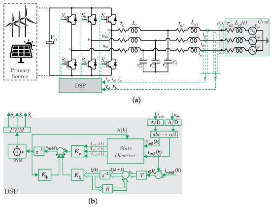
Figure 1. (a) Three-phase inverter connected to the grid by means of an LCL filter. (b) Details of the robust state feedback control based only on grid currents and voltages.

The grid is given by a series resistive-inductive structure. Nevertheless, for the purpose of control design and stability analysis, a predominantly inductive grid will be assumed here, since this condition represents the worst case for the performance of the grid current control loop [41]. Moreover, to encompass the uncertain and time-varying characteristic of the grid impedance typical in the scenario of weak grids, such as a microgrid applications [41], consider that the grid inductance $L_{g2}\left(t\right)$ is a time-varying parameter, belonging to a bounded interval where only the maximum and minimum values are given. Therefore, for a balanced three-phase system, one can write, for any of the three phases, that

$$L_g\left(t\right)=L_{g1}+L_{g2}\left(t\right)$$

(1)

where $L_g\left(t\right)\in$$[L_{gmin},L_{gmax}]$, $\forall t\ge 0$.

From the output voltage of the inverter, the plant in Figure 1 can be represented in state space by [21]

$$\dot{\mathit{x}}={\mathit{A}}_{abc}\left(L_g\left(t\right)\right){\mathit{x}}_{abc}+{{\mathit{B}}_{\mathit{u}}}_{abc}{\mathit{u}}_{abc}+{{\mathit{B}}_{\mathit{d}}}_{abc}\left(L_g\left(t\right)\right){\mathit{v}}_{dabc},$$

(2)

with matrices ${\mathit{A}}_{abc}\left(L_g\left(t\right)\right)$, ${{\mathit{B}}_u}_{abc}$ and ${{\mathit{B}}_d}_{abc}\left(L_g\left(t\right)\right)$ given by

$$\begin{array}{c}{\mathit{A}}_{abc}\left(L_g\left(t\right)\right)=\left[\begin{array}{ccc}{\mathbf{0}}_{3\times 3}& {\mathit{A}}_{p1}& {\mathbf{0}}_{3\times 3}\\ {\mathit{A}}_{p2}& {\mathbf{0}}_{3\times 3}& -{\mathit{A}}_{p2}\\ {\mathbf{0}}_{3\times 3}& {\mathit{A}}_{p3}& {\mathbf{0}}_{3\times 3}\end{array}\right];{{\mathit{B}}_u}_{abc}=\left[\begin{array}{c}-{\mathit{A}}_{p1}\\ {\mathbf{0}}_{3\times 3}\\ {\mathbf{0}}_{3\times 3}\end{array}\right];\hfill \\ {{\mathit{B}}_d}_{abc}\left(L_g\left(t\right)\right)=\left[\begin{array}{c}{\mathbf{0}}_{3\times 3}\\ {\mathbf{0}}_{3\times 3}\\ -{\mathit{A}}_{p3}\left(L_g\left(t\right)\right)\end{array}\right].\hfill \end{array}$$

(3)

Matrices ${\mathit{A}}_{p1}$, ${\mathit{A}}_{p2}$ and ${\mathit{A}}_{p3}\left(L_g\left(t\right)\right)$ are written as

$$\begin{array}{c}{\mathit{A}}_{p1}=\left[\begin{array}{ccc}-{\displaystyle \frac{2}{3L_c}}& {\displaystyle \frac{1}{3L_c}}& {\displaystyle \frac{1}{3L_c}}\\ {\displaystyle \frac{1}{3L_c}}& -{\displaystyle \frac{2}{3L_c}}& {\displaystyle \frac{1}{3L_c}}\\ {\displaystyle \frac{1}{3L_c}}& {\displaystyle \frac{1}{3L_c}}& -{\displaystyle \frac{2}{3L_c}}\end{array}\right];{\mathit{A}}_{p2}=\left[\begin{array}{ccc}{\displaystyle \frac{1}{C_f}}& 0& 0\\ 0& {\displaystyle \frac{1}{C_f}}& 0\\ 0& 0& {\displaystyle \frac{1}{C_f}}\end{array}\right];\hfill \\ {\mathit{A}}_{p3}\left(L_g\left(t\right)\right)=\left[\begin{array}{ccc}{\displaystyle \frac{2}{3L_g\left(t\right)}}& -{\displaystyle \frac{1}{3L_g\left(t\right)}}& -{\displaystyle \frac{1}{3L_g\left(t\right)}}\\ -{\displaystyle \frac{1}{3L_g\left(t\right)}}& {\displaystyle \frac{2}{3L_g\left(t\right)}}& -{\displaystyle \frac{1}{3L_g\left(t\right)}}\\ -{\displaystyle \frac{1}{3L_g\left(t\right)}}& -{\displaystyle \frac{1}{3L_g\left(t\right)}}& {\displaystyle \frac{2}{3L_g\left(t\right)}}\end{array}\right]\hfill \end{array}$$

(4)

The state vector ${\mathit{x}}_{abc}$, the control vector ${\mathit{u}}_{abc}$ and the disturbance vector ${\mathit{v}}_{gabc}$ are given by

$$\begin{array}{c}{\mathit{x}}_{abc}={\left[\begin{array}{ccccccccc}{i}_{ca}& i_{cb}& i_{cc}& v_{ca}& v_{cb}& v_{cc}& i_{ga}& i_{gb}& i_{gc}\end{array}\right]}^{{}^{\prime }}\hfill \\ {\mathit{u}}_{abc}={\left[\begin{array}{ccc}{u}_a& u_b& u_c\end{array}\right]}^{{}^{\prime }}\hfill \\ {\mathit{v}}_{dabc}={\left[\begin{array}{ccc}{v}_{ga}& v_{gb}& v_{gc}\end{array}\right]}^{{}^{\prime }}.\hfill \end{array}$$

(5)

Assuming a balanced three-phase system, the previous model can be rewritten from $abc$ to $\alpha \beta 0$ coordinates by means of the transformation [42]

$${\mathit{T}}_{\alpha \beta 0T}=\left[\begin{array}{ccc}{T}_{\alpha \beta 0}& 0_{3\times 3}& 0_{3\times 3}\\ 0_{3\times 3}& T_{\alpha \beta 0}& 0_{3\times 3}\\ 0_{3\times 3}& 0_{3\times 3}& T_{\alpha \beta 0}\end{array}\right],{\mathit{T}}_{\alpha \beta 0}={\displaystyle \frac{2}{3}}\left[\begin{array}{ccc}1& -\frac{1}{2}& -\frac{1}{2}\\ 0& \frac{\sqrt{3}}{2}& -\frac{\sqrt{3}}{2}\\ \frac{1}{2}& \frac{1}{2}& \frac{1}{2}\end{array}\right].$$

(6)

Applying the transformation (6) in model (2), one has

$$\begin{array}{c}{\dot{\mathit{x}}}_{\alpha \beta 0}\left(L_g\right)={\mathit{A}}_{\alpha \beta 0}\left(L_g\right){\mathit{x}}_{\alpha \beta 0}+{{\mathit{B}}_u}_{\alpha \beta 0}{\mathit{u}}_{\alpha \beta 0}+{\mathit{B}}_{d\alpha \beta 0}\left(L_g\right){\mathit{v}}_{d\alpha \beta 0}\hfill \end{array}$$

(7)

where the vectors and matrices in $\alpha \beta 0$ coordinates are given by

$$\begin{array}{c}{\mathit{x}}_{\alpha \beta 0}={\mathit{T}}_{\alpha \beta 0T}{\mathit{x}}_{abc}; \hspace{1em}\hspace{1em}\hspace{1em}{\mathit{A}}_{\alpha \beta 0}\left(L_g\right)={\mathit{T}}_{\alpha \beta 0T}{\mathit{A}}_{abc}\left(L_g\right){\mathit{T}}_{\alpha \beta 0T}^{-1}\hfill \\ {\mathit{u}}_{\alpha \beta 0}={\mathit{T}}_{\alpha \beta 0}{\mathit{u}}_{abc};\hspace{1em}\hspace{1em}\hspace{1em}\hspace{1em}{{\mathit{B}}_u}_{\alpha \beta 0}={\mathit{T}}_{\alpha \beta 0T}{\mathit{B}}_{uabc}{\mathit{T}}_{\alpha \beta 0}^{-1}\hfill \\ {\mathit{v}}_{d\alpha \beta 0}={\mathit{T}}_{\alpha \beta 0}{\mathit{v}}_{dabc}; \hspace{1em}\hspace{1em}\hspace{1em}{\mathit{B}}_{d\alpha \beta 0}\left(L_g\right)={\mathit{T}}_{\alpha \beta 0T}{\mathit{B}}_{dabc}\left(L_g\right){\mathit{T}}_{\alpha \beta 0}^{-1}\hfill \end{array}$$

(8)

Assuming a balanced system, and that there is no path for the current of axis ‘0’, the system can be described by means of two uncoupled single-phase systems, given by [42]

$$\begin{array}{c}{\dot{\mathit{x}}}_{\alpha }\left(t\right)=\mathit{A}\left(L_g\left(t\right)\right){\mathit{x}}_{\alpha }\left(t\right)+{\mathit{B}}_u{u}_{\alpha }\left(t\right)+{\mathit{B}}_d\left(L_g\left(t\right)\right)v_{g\alpha }\left(t\right)\hfill \\ {\dot{\mathit{x}}}_{\beta }\left(t\right)=\mathit{A}\left(L_g\left(t\right)\right){\mathit{x}}_{\beta }\left(t\right)+{\mathit{B}}_u{u}_{\beta }\left(t\right)+{\mathit{B}}_d\left(L_g\left(t\right)\right)v_{g\beta }\left(t\right)\hfill \end{array}$$

(9)

where

$$\begin{array}{c}\mathit{A}\left(L_g\left(t\right)\right)=\left[\begin{array}{ccc}-{\displaystyle \frac{r_c}{L_c}}& -{\displaystyle \frac{1}{L_c}}& 0\\ \\ {\displaystyle \frac{1}{C_f}}& 0& -{\displaystyle \frac{1}{C_f}}\\ \\ 0& {\displaystyle \frac{1}{L_g\left(t\right)}}& -{\displaystyle \frac{r_{g1}+r_{g2}}{L_g\left(t\right)}}\end{array}\right],{\mathit{B}}_u=\left[\begin{array}{c}{\displaystyle \frac{1}{L_c}}\\ 0\\ 0\end{array}\right],\hfill \\ \hfill \\ {\mathit{B}}_d\left(L_g\left(t\right)\right)=\left[\begin{array}{c}0\\ 0\\ {\displaystyle \frac{-1}{L_g\left(t\right)}}\end{array}\right],{\mathit{x}}_{\alpha }\left(t\right)=\left[\begin{array}{c}{i}_{c\alpha }\left(t\right)\\ v_{c\alpha }\left(t\right)\\ i_{g\alpha }\left(t\right)\end{array}\right],{\mathit{x}}_{\beta }\left(t\right)=\left[\begin{array}{c}{i}_{c\beta }\left(t\right)\\ v_{c\beta }\left(t\right)\\ i_{g\beta }\left(t\right)\end{array}\right]\hfill \end{array}$$

(10)

being, in this representation, $i_{c\alpha }$ the current through the converter-side inductor, $v_{c\alpha }$ the voltage across the filter capacitor, $i_{g\alpha }$ the current injected into the grid, $u_{\alpha }$ the control input and $v_{g\alpha }$ the grid voltage. The same reasoning is valid for axis $\beta$.

The following change of variables is adopted to represent the time-varying parameter $L_g\left(t\right)$ in terms of a polytopic model [18]

$${\theta }_1\left(t\right)=\frac{\frac{1}{L_g\left(t\right)}-\frac{1}{Lgmax}}{\frac{1}{Lgmin}-\frac{1}{Lgmax}},{\theta }_2\left(t\right)=1-{\theta }_1\left(t\right)$$

(11)

where $\left({\theta }_1\left(t\right),{\theta }_2\left(t\right)\right)\in \Theta ,\forall t\ge 0$, and

$$\Theta =\left\{\mathit{ϵ}\in {\mathbb{R}}^2:{ϵ}_1+{ϵ}_2=1,{ϵ}_1,{ϵ}_2\ge 0\right\}$$

(12)

In this case, parameter $1/L_g\left(t\right)$ appearing in matrices given in (10) can be replaced by

$$\begin{array}{c}\frac{1}{L_g\left(t\right)}=\left(\frac{1}{Lgmin}-\frac{1}{Lgmax}\right){\theta }_1\left(t\right)+\frac{1}{Lgmax}=\frac{1}{Lgmin}{\theta }_1\left(t\right)+\frac{1}{Lgmax}{\theta }_2\left(t\right)\hfill \end{array}$$

(13)

After multiplying the terms not depending on $L_g\left(t\right)$ by ${\theta }_1\left(t\right)+{\theta }_2\left(t\right)$ (homogenization procedure), matrices $\mathit{A}\left(L_g\left(t\right)\right)$ and ${\mathit{B}}_d\left(L_g\left(t\right)\right)$ in (3) can be rewritten in the form

$$\begin{array}{c}\mathit{A}\left(L_g\left(t\right)\right)=\mathit{A}\left(\mathit{\theta }\left(t\right)\right)={\theta }_1\left(t\right){\mathit{A}}_1+{\theta }_2\left(t\right){\mathit{A}}_2,\hfill \\ \hfill \\ {\mathit{B}}_d\left(L_g\left(t\right)\right)={\mathit{B}}_d\left(\mathit{\theta }\left(t\right)\right)={\theta }_1\left(t\right){\mathit{B}}_{d_1}+{\theta }_2\left(t\right){\mathit{B}}_{d_2}\hfill \end{array}$$

(14)

i.e., in terms of a polytopic description, where ${\mathit{A}}_1=\mathit{A}\left(L_{gmin}\right)$, ${\mathit{A}}_2=\mathit{A}\left(L_{gmax}\right)$, ${\mathit{B}}_{d1}={\mathit{B}}_d\left(L_{gmin}\right)$ and ${\mathit{B}}_{d2}={\mathit{B}}_d\left(L_{gmax}\right)$.

For the application of a digital control law, consider the discretization of the plant with a sufficiently small sampling period $T_s$, and also the inclusion of an additional state, $\varphi$, representing the one sample digital delay. From this point on, for simplicity, the subscripts $\alpha$ and $\beta$ are suppressed. The discretized model is given by

$$\begin{array}{c}\mathit{x}(k+1)={\mathit{A}}_d\left(\mathit{\theta }\left(k\right)\right)\mathit{x}\left(k\right)+{\mathit{B}}_{ud}\left(\mathit{\theta }\left(k\right)\right)\varphi \left(k\right)+{\mathit{B}}_{dd}\left(\mathit{\theta }\left(k\right)\right)v_g\left(k\right)\hfill \\ \varphi (k+1)=u\left(k\right)\hfill \\ y\left(k\right)={\mathit{C}}_y\mathit{x}\left(k\right)=\left[001\right]\mathit{x}\left(k\right)=i_g\left(k\right)\hfill \end{array}$$

(15)

To ensure tracking of sinusoidal references and rejection of harmonic disturbances, n resonant controllers are included in the model, leading to the representation [21]

$$\begin{array}{c}\begin{array}{c}\mathit{\xi }(k+1)=\mathit{R}\mathit{\xi }\left(k\right)+\mathit{T}(i_{ref}\left(k\right)-y\left(k\right))\hfill \end{array}\hfill \end{array}$$

(16)

where

$$\mathit{\xi }=\left[\begin{array}{c}{\mathit{\xi }}_1\\ ⋮\\ {\mathit{\xi }}_n\end{array}\right],\mathit{R}=\left[\begin{array}{ccc}{\mathit{R}}_1& & \\ & \ddots & \\ & & {\mathit{R}}_n\end{array}\right],\mathit{T}=\left[\begin{array}{c}{\mathit{T}}_1\\ ⋮\\ {\mathit{T}}_n\end{array}\right]$$

(17)

and $i_{ref}$ is the reference for the grid currents. $\mathit{\xi }$, $\mathit{R}$ and $\mathit{T}$ are, respectively, the state vector and the matrices of the multiple resonant controllers. Each vector ${\mathit{\xi }}_i$, $i=1\cdots n$, has two states and represent one resonant controller.

Notice that (15) and (16) can be rewritten as

$$\begin{array}{c}\left[\begin{array}{c}\mathit{x}(k+1)\\ \varphi (k+1)\\ \mathit{\xi }(k+1)\end{array}\right]=\left[\begin{array}{ccc}{\mathit{A}}_d\left(\mathit{\theta }\left(k\right)\right)& {\mathit{B}}_{ud}\left(\mathit{\theta }\left(k\right)\right)& {\mathbf{0}}_{3\times 2n}\\ {\mathbf{0}}_{1\times 3}& 0& {\mathbf{0}}_{1\times 2n}\\ -{\mathit{T}}_{2n\times 1}{\mathit{C}}_y& {\mathbf{0}}_{2n\times 1}& {\mathit{R}}_{2n\times 2n}\end{array}\right]\left[\begin{array}{c}\mathit{x}\left(k\right)\\ \varphi \left(k\right)\\ \mathit{\xi }\left(k\right)\end{array}\right]+\hfill \\ \hfill \\ +\left[\begin{array}{c}{\mathbf{0}}_{3\times 1}\\ 1\\ {\mathbf{0}}_{2n\times 1}\end{array}\right]u\left(k\right)+\left[\begin{array}{c}{\mathit{B}}_{dd}\left(\mathit{\theta }\left(k\right)\right)\\ 0\\ {\mathbf{0}}_{2n\times 1}\end{array}\right]v_g\left(k\right)+\left[\begin{array}{c}{\mathbf{0}}_{3\times 1}\\ 0\\ {\mathit{T}}_{2n\times 1}\end{array}\right]i_{ref}\left(k\right)\hfill \end{array}$$

(18)

or, in a more compact form, as

$$\begin{array}{c}\begin{array}{c}\mathit{\rho }(k+1)=\mathit{G}\left(\mathit{\theta }\left(k\right)\right)\mathit{\rho }\left(k\right)+{\mathit{H}}_{u}u\left(k\right)+{\mathit{H}}_d\left(\mathit{\theta }\left(k\right)\right)v_g\left(k\right)+{\mathit{H}}_{ref}{i}_{ref}\left(k\right)\hfill \end{array}\hfill \\ \hfill \\ y\left(k\right)=\mathit{C}\mathit{\rho }\left(k\right),\mathit{C}=\left[\begin{array}{cc}{\mathit{C}}_y& {\mathbf{0}}_{1\times (2n+1)}\end{array}\right]\hfill \end{array}$$

(19)

where

$$\begin{array}{c}\mathit{G}\left(\mathit{\theta }\left(k\right)\right)={\displaystyle \sum _{j=1}^2}{\theta }_j\left(k\right){\mathit{G}}_j,{\mathit{H}}_d\left(\mathit{\theta }\left(k\right)\right)={\displaystyle \sum _{j=1}^2}{\theta }_j\left(k\right){\mathit{H}}_{dj}\\ \end{array}$$

(20)

with ${\mathit{G}}_1=\mathit{G}\left(L_{gmin}\right)$, ${\mathit{G}}_2=\mathit{G}\left(L_{gmax}\right)$, ${\mathit{H}}_{d1}={\mathit{H}}_d\left(L_{gmin}\right)$, ${\mathit{H}}_{d2}={\mathit{H}}_d\left(L_{gmax}\right)$, and $[{\theta }_1\left(k\right),{\theta }_2\left(k\right)]$$\in \Theta$, $\forall k\ge 0$.

Consider now that the parameters ${\theta }_j\left(k\right)$ can vary in time respecting the bounds

$$\left|{\theta }_j(k+1)-{\theta }_j\left(k\right)\right|\le b,j=1,2$$

(21)

If b tends to 1, the parameters have arbitrarily fast rates of variation. On the other hand, if b approaches zero, the parameters become time-invariant. Therefore, the polytopic model of the augmented system (19), with the constraints in (20), allows to investigate the stability under bounded rates of parametric variation in the grid inductance.

The model in (19) and (20) can be used to obtain the gains of state feedback controllers by means of LMIs. Due to the convexity of this polytopic representation, LMIs tested only at the vertices are capable to ensure stability and performance for an entire set of uncertainties. This property makes LMI conditions very attractive from the computational point of view, avoiding the need of exhaustive griding techniques to investigate stability and performance, which cannot conclude with theoretical guarantees for the case of time-varying parameters [18,22,23,43].

One drawback with state feedback control techniques is the need to measure all the state variables, which increases the cost and the complexity of the system, besides potentially increasing reliability issues associated with sensor fault-through capacity of the system [26]. In this context, the use of state observers become an important alternative. Nevertheless, when parametric uncertainties must be taken into account, the problem to provide robustness to controllers based on observed states becomes more challenging, and new strategies to combine robust state feedback control with robust state observation are still one point for investigation [29,44].

In this scenario, this paper provides a contribution to the LMI based design for observer-based robust controllers applied to grid-connected converters with LCL filters, as detailed in the next section.

3. Proposed Design Based on LMIs

As a performance criterium to guide the design of the control and observer gains, consider that, using the LMI-framework, it is possible to ensure that all the closed-loop poles of an uncertain discrete-time system are located inside the region $\mathcal{C}\left(r\right)$, defined by the circle of radius r and center at the origin of the complex plane, as can be seen in Figure 2.

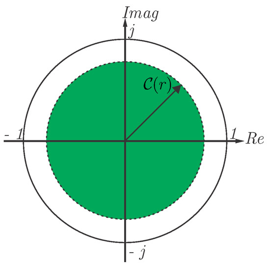
Figure 2. Region $\mathcal{C}\left(r\right)$, for pole location.

The radius r provide an upper bound for the settling time ($t_s$) of the uncertain system transient responses [45], as given by

$$t_s\le \frac{4T_s}{\left|ln\right(r\left)\right|}$$

(22)

In the sequence, the main contribution of this work is presented, comprised by a systematic procedure based on LMIs to compute off-line the sets of gains for the controller and observer, including a new theoretical certificate of stability for grid-connected converters operating under grid inductance variations. Note that, for each design, only a single real parameter r, limited between 0 and 1, needs to be chosen.

3.1. Robust Control Design

From (19), consider the state feedback control law

$$u\left(k\right)=\mathit{K}\mathit{\rho }\left(k\right)=\left[\begin{array}{ccc}{\mathit{K}}_x& K_{\varphi }& {\mathit{K}}_{\xi }\end{array}\right]\left[\begin{array}{c}\mathit{x}\left(k\right)\\ \varphi \left(k\right)\\ \mathit{\xi }\left(k\right)\end{array}\right]$$

(23)

The controller gains can be computed using a robust pole location condition based on LMIs. Therefore, for a chosen radius $0<r_c<1$, if there exist matrices $0<{𝓢}_j={𝓢}_j^{\prime }\in {\mathbb{R}}^{(4+2n)\times (4+2n)}$, $𝓖\in {\mathbb{R}}^{(4+2n)\times (4+2n)}$ and $𝓡\in {\mathbb{R}}^{1\times (4+2n)}$ that solve the following LMIs (n represent the number of resonant controllers, that is, if four resonant controller is used, and $n=4$ then $\mathit{K}$ belongs to ${\mathcal{R}}^{1\times 12}$.)

$$\begin{array}{c}\left[\begin{array}{cc}𝓖+{𝓖}^{\prime }-{𝓢}_j& {𝓖}^{\prime }\frac{{\mathit{G}}_j^{{}^{\prime }}}{r_c}+{𝓡}^{\prime }\frac{{\mathit{H}}_u^{{}^{\prime }}}{r_c}\\ \frac{{\mathit{G}}_j}{r_c}𝓖+\frac{{\mathit{H}}_u}{r_c}𝓡& {𝓢}_i\end{array}\right]>0\begin{array}{c}i=1,2\\ j=1,2\end{array}\hfill \end{array}$$

(24)

then the state feedback control gain given by

$$\mathit{K}=𝓡{𝓖}^{-1}$$

(25)

ensures: (i) closed-loop robust stability of (19) for all $[{\theta }_1\left(k\right),{\theta }_2\left(k\right)]\in \Theta$; (ii) that all the closed-loop poles for $\mathit{G}\left(\theta \left(k\right)\right)+{\mathit{H}}_u\mathit{K}$ are located inside the circle $\mathcal{C}\left(r_c\right)$; (iii) the tracking of sinusoidal references for the grid current and rejection of harmonics in the grid voltage, due the resonant controllers [21].

3.2. Observer Design and Implementation

Consider the state observer given by

$$\begin{array}{c}\widehat{\mathit{x}}(k+1)={\mathit{A}}_{do}\widehat{\mathit{x}}\left(k\right)+{\mathit{B}}_{uo}\varphi \left(k\right)+{\mathit{B}}_{do}{v}_{go}\left(k\right)+\Gamma {\mathit{C}}_y(\mathit{x}\left(k\right)-\widehat{\mathit{x}}\left(k\right))\hfill \end{array}$$

(26)

where $\widehat{\mathit{x}}={\left[{\widehat{i}}_c{\widehat{v}}_c{\widehat{i}}_g\right]}^{\prime }$ is the observed states vector, $\Gamma$ is the observer gains vector, and $v_{go}$ is grid voltage estimation, used here since the actual voltage $v_g$ is not available in practice.

To implement the observer in (26), the designer must choose a fixed value $L_{go}\in [L_{gmin},L_{gmax}]$. It is not necessary to identify this parameter with more complex strategies, but only choosing one value of $L_{go}$ in the interval above. Then, the observer matrices ${\mathit{A}}_{do}$, ${\mathit{B}}_{uo}$ and ${\mathit{B}}_{do}$ are computed according to this choice based in (14)–(15). Since ${\mathit{A}}_{do}$, ${\mathit{B}}_{uo}$, ${\mathit{B}}_{do}$ and the gains are not updated in real time, the practical implementation of the observer in (26) is simple, and can ensure suitable closed-loop responses by the proper design of $\Gamma$, as will be confirmed in Section 4 and Section 5.

The observer gains can also be computed by means of LMIs. In this sense, for a chosen radius $0<r_o<1$, if there exist matrices $0<{𝓢}_j={𝓢}_j^{\prime }\in {\mathbb{R}}^{3\times 3}$, $𝓖\in {\mathbb{R}}^{3\times 3}$ and $𝓡\in {\mathbb{R}}^{1\times 3}$ that solve the following LMIs

$$\left[\begin{array}{cc}𝓖+{𝓖}^{\prime }-{𝓢}_j& {𝓖}^{\prime }\frac{{\mathit{A}}_{dj}}{r_o}+{𝓡}^{\prime }\frac{{\mathit{C}}_y}{r_o}\\ \frac{{\mathit{A}}_{dj}^{{}^{\prime }}}{r_o}𝓖+\frac{{\mathit{C}}_y^{{}^{\prime }}}{r_o}𝓡& {𝓢}_i\end{array}\right]>0,\begin{array}{c}i=1,2\\ j=1,2\end{array}$$

(27)

then the robust observer gain given by

$${\Gamma }^{\prime }=𝓡{𝓖}^{-1}$$

(28)

ensures that the observer is robustly stable for all $[{\theta }_1\left(k\right),{\theta }_2\left(k\right)]\in \Theta$, and that all the closed-loop poles of ${\mathit{A}}_d\left(\mathit{\theta }\left(k\right)\right)+\Gamma {\mathit{C}}_y$ are located inside the circle with center at zero and radius $r_o$.

In comparison to (24), the observer design using (27) is based on the duality between controller and observer, replacing the state matrix by its transpose and the control input matrix by the transpose of the output matrix (see Appendix A for details) [46].

In order to have an estimate of $v_{go}$ to implement the observer, first note that the voltage at the PCC can be modeled in stationary reference frame based on the Kirchhoff’s voltage law, and written as a function of the state vector, given by

$$v_{PCC}\left(k\right)={\mathit{C}}_p\left(\mathit{\theta }\left(k\right)\right)\mathit{x}\left(k\right)+D_p\left(\mathit{\theta }\left(k\right)\right)v_g\left(k\right)$$

(29)

with

$$\begin{array}{c}{\mathit{C}}_p\left(\mathit{\theta }\left(k\right)\right)={\theta }_1\left(k\right){\mathit{C}}_p\left(L_{gmin}\right)+{\theta }_2\left(k\right){\mathit{C}}_p\left(L_{gmax}\right)\hfill \\ {\mathit{D}}_p\left(\mathit{\theta }\left(k\right)\right)={\theta }_1\left(k\right)D_p\left(L_{gmin}\right)+{\theta }_2\left(k\right)D_p\left(L_{gmax}\right)\hfill \end{array}$$

(30)

where

$$\begin{array}{c}{\mathit{C}}_p\left(L_g\left(k\right)\right)=\left[\begin{array}{ccc}0& \frac{L_{g2}\left(k\right)}{L_g\left(k\right)}& \frac{r_{g2}{L}_{g1}-r_{g1}{L}_{g2}\left(k\right)}{L_g\left(k\right)}\end{array}\right]\hfill \\ D_p\left(L_g\left(k\right)\right)=\begin{array}{c}1-\frac{L_{g2}\left(k\right)}{L_g\left(k\right)}\end{array}\hfill \end{array}$$

(31)

Based on (29), the voltage $v_{go}$, used in the observer Equation (26), can be calculated from the observed states $\widehat{\mathit{x}}\left(k\right)$ and the measurement of $v_{PCC}\left(k\right)$, according to

$$v_{go}\left(k\right)=-D_{po}^{-1}{\mathit{C}}_{po}\widehat{\mathit{x}}\left(\mathit{k}\right)+D_{po}^{-1}{v}_{PCC}\left(k\right)$$

(32)

In (32), $D_{po}$ is a fixed scalar and ${\mathit{C}}_{po}$ is a fixed vector, obtained off-line from (31), for the same $L_{go}$ chosen to compute the matrices in (26). From (1) and (31), notice that $D_{po}$ is always invertible for $L_{g1}\ne 0$.

3.3. Robust Stability Analysis Based on Less Conservative LMIs

A robust stability analysis of the system with feedback of the observed states is now in order. For that, consider the implementation of the control law (23), with the feedback of the observed states instead of the real states, leading to

$$u\left(k\right)={\mathit{K}}_x\widehat{\mathit{x}}\left(k\right)+K_{\varphi }\varphi \left(k\right)+{\mathit{K}}_{\xi }\mathit{\xi }\left(k\right)$$

(33)

From the augmented system (18), including the observer (26), the control law (33), and also taking into account Equation (32), the closed-loop system can be written as

$$\begin{array}{c}\left[\begin{array}{c}\mathit{x}(k+1)\\ \varphi (k+1)\\ \mathit{\xi }(k+1)\\ \widehat{\mathit{x}}(k+1)\end{array}\right]=\underset{{\mathit{A}}_{cl}\left(\mathit{\theta }\left(k\right)\right)}{\underbrace{\left[\begin{array}{cccc}{\mathit{A}}_d\left(\mathit{\theta }\left(k\right)\right)& {\mathit{B}}_{ud}\left(\mathit{\theta }\left(k\right)\right)& \mathbf{0}& \mathbf{0}\\ \mathbf{0}& K_{\varphi }& {\mathit{K}}_{\mathit{\xi }}& {\mathit{K}}_{\mathit{x}}\\ -\mathit{T}{\mathit{C}}_y& 0& \mathit{R}& \mathbf{0}\\ {𝓜}_1\left(\mathit{\theta }\left(k\right)\right)& {\mathit{B}}_{\mathit{uo}}& \mathbf{0}& {𝓜}_2\end{array}\right]}}\left[\begin{array}{c}\mathit{x}\left(k\right)\\ \varphi \left(k\right)\\ \mathit{\xi }\left(k\right)\\ \widehat{\mathit{x}}\left(k\right)\end{array}\right]\hfill \\ +\left[\begin{array}{c}\mathbf{0}\\ 0\\ \mathit{T}\\ \mathbf{0}\end{array}\right]i_{ref}\left(k\right)+\left[\begin{array}{c}{\mathit{B}}_{\mathit{dd}}\left(\mathit{\theta }\left(k\right)\right)\\ 0\\ \mathbf{0}\\ {\mathit{B}}_{\mathit{do}}{D}_{po}^{-1}{D}_p\left(\mathit{\theta }\left(k\right)\right)\end{array}\right]v_g\left(k\right)\hfill \end{array}$$

(34)

with

$$\begin{array}{c}{𝓜}_1\left(\mathit{\theta }\left(k\right)\right)=\Gamma {\mathit{C}}_y+{\mathit{B}}_{do}{D}_{po}^{-1}{\mathit{C}}_p\left(\mathit{\theta }\left(k\right)\right)\hfill \\ {𝓜}_2={\mathit{A}}_{do}-\Gamma {\mathit{C}}_y-{\mathit{B}}_{do}{D}_{po}^{-1}{\mathit{C}}_{po}\hfill \end{array}$$

(35)

To certify the robust stability of ${\mathit{A}}_{cl}\left(\mathit{\theta }\left(k\right)\right)$ in (34), consider the condition solvable in terms of LMIs given in the Appendix B, which rely on a parameter-dependent Lyapunov function for the closed-loop system. These LMIs can provide less conservative evaluations of stability due to the extra matrix variables and the polynomial relaxations, allowing to provide a bound b for the maximum allowed variation rates of $\mathit{\theta }\left(k\right)$. This feature allows us to certify the stability under time-varying parameters in cases where the polyquadratic LMIs [40] extensively used in the literature for grid-connected converters may be conservative, as will be shown in Section 6.

Remark 1. 

Notice the design in Section III.B provides observer gains which ensure that all the transient responses of (26) are bounded by $r_o^k$ (decay rate). Moreover, due to the polyquadratic stability in (27) [40], one has the stability of the observer (26) for any ${\mathit{A}}_{do}$ belonging to ${\mathit{A}}_d\left(\mathit{\theta }\left(k\right)\right)$, for arbitrary time-varying parameters in the plant matrices inside the previously given polytopes. Section III.C certifies the stability of the system with feedback of the observed states for the entire range of parameters in the case of time-varying grid parameters.

Remark 2. 

The observer could be implemented using directly the measured value of $v_{PCC}$, avoiding the need of estimating $v_{go}$. On the other hand, the drawback is that the designer no longer can choose $A_{do}$, $B_{uo}$ and $B_{do}$ considering different values for $L_{go}$, since these matrices would depend only on the LCL filter parameters. Therefore, the estimation error only will converge to zero when the grid inductance $L_{g2}$ approaches 0 mH, i.e., the observation of the states tends to be impaired in weaker grid conditions.

Remark 3. 

When compared with state feedback controllers which measure the inverter-side currents, the voltage across the capacitor filters, and the grid currents [20,21,22,23,37,38], the proposed approach only demands the measurement of the grid currents, keeping stability and performance, demanding a lower hardware cost of implementation. When compared with conventional proportional-resonant controllers [47,48], the proposed approach demands the same hardware cost, but with the advantage of using robust state feedback controllers from the literature, which allows dealing with an arbitrary number of resonant controllers, representing an advantage in terms of a better trade-off between transient and steady state performances. When compared with other works which deal with robust observers [25,27,28,29,30,31,32,33], the approach in the paper provides a parameter-dependent Lyapunov function constructed with a very high computational efficiency, based on the solution of a set of LMIs that was not explored in power electronics literature yet, certifying the stability of the closed-loop system under parametric variations of the grid impedance.

Remark 4. 

Concerning stability analyses, the proposed approach first ensures the robust stability of the observer designed by LMIs (27) and (28) (see Appendix A for proof). Then, the stability of the complete closed-loop system, (34), is ensured by the feasibility of the LMIs (A1) (see Appendix B for proof).

A summary of the proposed procedure is given in the sequence, which can be executed off-line and in a fast way using the LMI Control Toolbox from MATLAB.

Summary with the steps of the proposed procedure.

•Design of control and observer gains (executed off-line):

1: choose $r_c$ and solve the LMIs in (24) to obtain control gain $\mathit{K}$;

2: choose $r_o$ and solve the LMIs in (27) to obtain

observer gain $\Gamma$ in (28);

3: choose a fixed value $L_{go}\in [L_{gmin},L_{gmax}]$, compute ${\mathit{A}}_{do}$, ${\mathit{B}}_{uo}$ and ${\mathit{B}}_{do}$

and certify the robust stability of ${\mathit{A}}_{cl}\left(\mathit{\theta }\left(k\right)\right)$ in (34) by means of

the LMIs (A1) in Appendix B.

4. Design Example: Case Study

Consider the plant in Figure 1, with augmented model in (18), and with parameters given in Table 1. The grid inductance interval was borrowed from [21,22], to represent the uncertainty in this parameter.

Table 1. System parameters.

Converter inductance $L_c$	1 mH
Filter capacitor $C_f$	62 $\mathsf{\mu }$H
Grid-side inductance $L_{g1}$	0.3 mH
Interval for the grid inductance	[0 mH; 1 mH]
Sampling frequency $T_s$	1/20,040 s
Switching frequency	1/10,020 s
Grid phase voltage	127 Vrms; 60 Hz
DC-link	400 V
Resonant frequencies	60, 180, 300 and 420 Hz
Resonant damping factor	0.0001

A resonant controller is included at 60 Hz (fundamental frequency) and also at the $3\mathrm{rd}$, $5\mathrm{th}$ and $7\mathrm{th}$ harmonics, to ensure rejection of disturbances from the grid voltages at these frequencies. Notice that the formulation in Section 3 assumes $i_g$ as a measured variable. In this case, the observability matrix of the plant for the parameters in Table 1 exhibits full rank of columns for the entire interval from $L_{gmin}$ to $L_{gmax}$, indicating observability.

To fulfill step 1 of the proposed design procedure, the controller gains are computed by means of the robust pole location conditions. Taking into account (22), $r_c=0.999$ is chosen as the bound of decay rate for the transient responses, resulting in the gains (truncated with 4 decimal digits)

$$\mathit{K}\left(P_{loc}\right)=\left[\begin{array}{c}-9.2382-1.599-0.0239-0.4291\cdots \hfill \\ \cdots 45.0233-44.431315.8166-15.4541\cdots \hfill \\ \cdots 9.1919-9.38515.0822-5.6989\hfill \end{array}\right]$$

(36)

In step 2, to compute the robust state observer gains, the bound of decay rate was chosen as $r_o=0.93$, so that the observer has sufficiently fast dynamic responses. Solving the LMIs (27) for this parameter, one has the observer gains (In terms of computational time, the LMIs (24) provide control gains within 600 ms, while the LMIs (27) provide observer gains in about 60 ms, using a notebook with Core i7 processor and 8 GB of RAM.)

$${\Gamma }^{\prime }=\left[0.32264.67341.4405\right]$$

(37)

Following step 3, the condition $L_{go}=L_{gmax}$ is chosen to obtain the fixed observer matrices. Then, to certify the robust stability of the closed-loop system with the feedback of the observed states, matrix ${\mathit{A}}_{cl}\left(\mathit{\theta }\left(k\right)\right)$ in (34) is computed. For the controller $\mathit{K}\left(P_{loc}\right)$ in (36) and the observer gains in (37), the dynamic matrix of the augmented system, ${\mathit{A}}_{cl}\left(\mathit{\theta }\left(k\right)\right)$, can be proven robustly stable for $b=1$, using the LMIs in Appendix B. In other words, the system is robustly stable for slow or arbitrarily fast variations of $L_g$ inside the interval from $L_{gmin}$ to $L_{gmax}$ chosen for this design (i.e., from $0.3$ mH to $1.3$ mH).

Figure 3 and Figure 4 allow to evaluate the performance of the closed-loop system with feedback of the observed states and gains obtained with the proposed procedure.

Figure 3. Closed-loop system with control gain $\mathit{K}\left(P_{loc}\right)$ in (36) and robust observer with gains given in (37): (a) Eigenvalues for a sweep in $L_g$ from $L_{gmin}$ to $L_{gmax}$. (b) Bode diagrams of magnitude: from $i_{ref}$ to $i_g$ (top) and from $v_g$ to $i_g$ (bottom) for values of $L_g$ in the interval of uncertainty.

Figure 4. Simulation results with controller $\mathit{K}\left(P_{loc}\right)$ in (36) and robust observer (37). Reference ($i_{g\alpha ref}$) and output ($i_{g\alpha }$) for: (a) minimum grid inductance; (b) maximum grid inductance; (c) variations of grid inductance from $L_{gmin}$ to $L_{gmax}$ and vice versa, at the times indicated by the arrows.

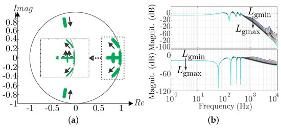
First, to corroborate the stability, Figure 3a shows the eigenvalues of the closed-loop system, including controller and observer, for a fine discretization in $L_g$. The arrows illustrate the movement of the eigenvalues for a sweep from $L_{gmin}$ to $L_{gmax}$. All eigenvalues of ${\mathit{A}}_{cl}\left(\mathit{\theta }\left(k\right)\right)$ belong to the unit circle, indicating robust stability for the entire range of parameters. The robust stability under time-varying parameters is proven in step 3 of the procedure, based on the parameter-dependent Lyapunov function in Appendix B.

Regarding to frequency responses, Figure 3b(top) illustrates the responses from the reference to the grid currents. One can verify the gain of 0 dB at the frequency of 60 Hz, which indicates the steady state capacity of the closed-loop system to track with small errors sinusoidal references at this frequency. Figure 3b(bottom) illustrates the frequency responses from the grid voltages to the grid currents, from which one can verify good disturbance rejection at 60 Hz and at the chosen odd harmonics, for all values of $L_g$ in the interval of uncertainty.

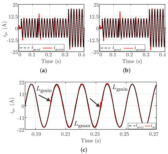
Figure 4 and Figure 5 show the simulations of the system carried out in software PSIM. In the simulation the inverter is based on IGBTs, the DC bus has 400 V, an ideal LCL filter is used, and sinusoidal sources are used to represent the grid. A Dyncamic Link Library (DLL) block programmed in C++ is used to implement the control algorithm. The control signals are bounded in +/−400 V and and a space vector modulation (SVM) is used to generate the signals to command the IGBTs. A deadtime is used to avoid short circuit in the inverter. The synchronization algorithm used here is a Kalman filter [49], which allow to generate the grid current references $i_{\alpha }$ and $i_{\beta }$, to simulate active or reactive power injection into the grid.

Figure 5. Simulation results of the closed-loop system with controller $K^{\prime }\left(P_{loc}\right)$ in (36) and conventional observer (38). Reference ($i_{g\alpha ref}$) and output ($i_{g\alpha }$) for: (a) minimum grid inductance. (b) maximum grid inductance. (c) Eigenvalues of the closed-loop system indicating instability.

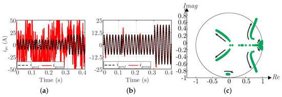
Figure 4a,b illustrate simulation results for the closed-loop system with feedback of the observed states, and operation with the extreme values of the grid inductance. For both conditions, the results confirm reference tracking with suitable transient and steady state performances under reference variations encompassing phase and amplitude changes. The first transient, at $t=0.01$ s, represents the start of the injection of reactive-capacitive power into the grid, followed by a variation to reactive-inductive power injection, at $t=0.1$ s, and then to active power injection, at $t=0.2$ s. At $t=0.3$ s, the active power injected into the grid goes from $50\%$ to $100\%$ of the nominal power. Figure 4c shows the $\alpha$ axis closed-loop responses for sudden variations of inductance from $L_{gmin}$ to $L_{gmax}$, at the first arrow, and from $L_{gmax}$ to $L_{gmin}$, at the second arrow. One can notice that the system remains stable under grid impedance variations, with suitable transient performance, as expected from the stability certificate provided by step 3 of the proposed procedure.

Comparison with Nonrobust Observer

To demonstrate the importance of a robust state observer design, a comparison with a nonrobust observer is developed. The nonrobust observer is conventionally designed here by means of the function place from MATLAB, choosing the maximum grid inductance as a nominal plant, and locating the eigenvalues of the state matrix at the positions 0.1, 0.3 and 0.5. These choices lead to the nonrobust observer gains given by

$${\Gamma }^{\prime }=\left[1.80895.79131.9285\right]$$

(38)

The tests shown in Figure 3a and Figure 4a,b are repeated now for the nonrobust observer, leading to the results in Figure 5. One can clearly notice the instability for the operation with minimum grid inductance, corroborating the importance of a robust observer design. Figure 5c explains the unstable behavior with the nonrobust observer, due to the closed-loop eigenvalues outside the unit circle, for values of grid inductance in the interval $[0,1]$ mH.

Notice that the design of other nonrobust observers (i.e., designed for different sets of nominal parameters) could be carried out, but the stability would not be guaranteed in the stage of the computation of the observer gains, and would still have to be tested after the design for the entire range of parameters. Moreover, even if the design of the nonrobust observer ensures all closed-loop eigenvalues inside the unit circle, this is only a necessary condition for the stability under time-varying grid parameters. On the other hand, the proposed procedure can provide in a fast way, by means of LMIs, the observer gains and a theoretical certificate of stability also for time-varying parameters.

5. Experimental Results

The aim of this section is to demonstrate the practical viability of the proposed robust observer for the control of an inverter connected to a real grid.

The experimental results were obtained using the prototype shown in Figure 6, which has a nominal power of 5.4 kW, encompassing a three-phase full-bridge inverter based on IGBTs, and a three-phase LCL filter with parameters given in Table 1. The control law is implemented in the digital signal processor (DSP) TMS320F28335, following the block diagram shown in Figure 1. The closed-loop system is connected to a public distribution grid, with uncertain grid inductance, belonging to the interval given in Table 1. The grid voltages are given in Figure 7a, and are affected by harmonics, as shown Figure 7b. The synchronization with the PCC voltage is obtained by means of a Kalman filter [49]. The results in $\alpha \beta$ presented in the sequence were obtained experimentally, from the DSP data.

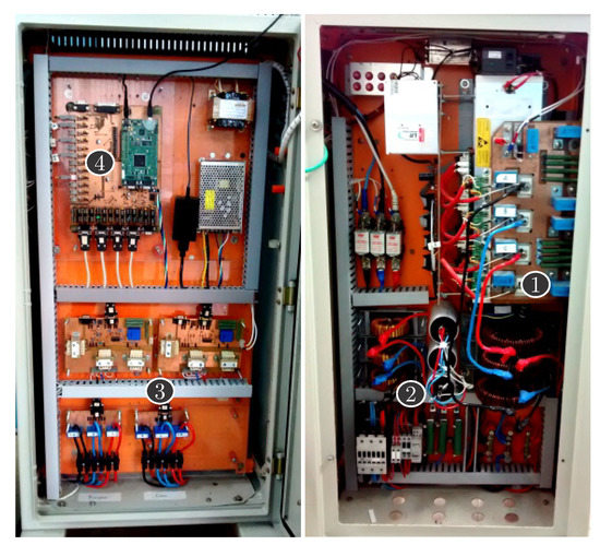
Figure 6. Experimental prototype encompassing the three-phase inverter (1), LCL filter (2), sensors (3) and DSP (4) used for control.

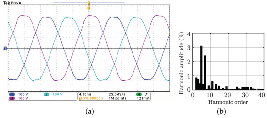
Figure 7. Experimental results: (a) distorted grid line-to-line voltages; (b) harmonic spectrum for the line-to-line voltage in channel 1 of (a).

Figure 8 shows the LCL filter states in $\alpha \beta$ coordinates for a test of reference tracking for a similar reference pattern as the one described in Figure 4, using the feedback of the observed states, with control gains $\mathit{K}$($P_{loc}$) in (36) and observer gains (37). These results confirm good correspondence of the measured variables ($i_c$, $i_g$, $v_c$) with the respective observed ones (${\widehat{i}}_c$, ${\widehat{i}}_g$, ${\widehat{v}}_c$), for both $\alpha$ and $\beta$ axes, with good transient and steady state performances. It should be recalled that, in this test, the measurements of the converter-side currents and the capacitor voltages of the filter were not used in the computation of the control signal. These variables were measured and then transformed to $\alpha \beta$ coordinates only to experimentally validate the proposed observer.

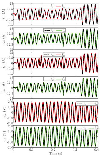
Figure 8. Experimental results for variables in $\alpha \beta$ axes: measured states ($i_{c\alpha \beta }$, $i_{g\alpha \beta }$ and $v_{c\alpha \beta }$) and respective observed states (${\widehat{i}}_{c\alpha \beta }$, ${\widehat{i}}_{g\alpha \beta }$ and ${\widehat{v}}_{c\alpha \beta }$).

Figure 9a presents, with better detail, the grid-injected currents in $\alpha \beta$ coordinates, from Figure 8, confirming that the closed-loop system can properly track sinusoidal references and reject disturbances from the public distribution grid, as expected by the frequency responses in Figure 3b. It is also important to notice that even in the case there is a residual observation error, the tracking error will converge to zero due to the asymptotic stability of the dynamic matrix in (34) and to the resonant controllers.

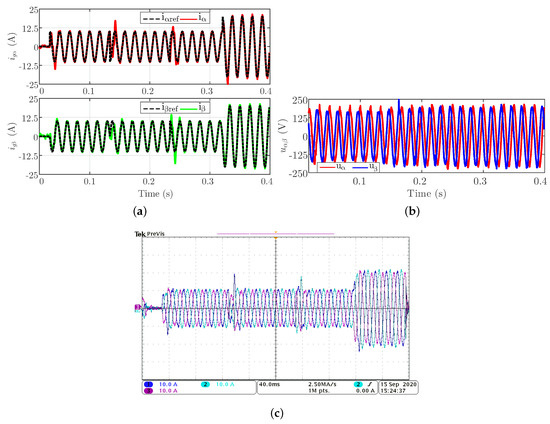
Figure 9. Experimental results for the reference variation test: (a) reference and output current for the closed-loop system for the $\alpha$ axis (top); and the $\beta$ axis (bottom). (b) control actions in $\alpha \beta$ axis and (c) Three-phase grid currents.

Moreover, the waveforms in Figure 9a confirm suitable transient recovers in the occurrence of phase and amplitude variations of the references, as expected by the simulations on Figure 4a,b, obtained with similar reference profiles. This also indicates that the uncertainty interval used for grid inductances in the control and observer designs is adequate to cope with the conditions found in this experimental evaluation.

Figure 9b shows the three-phase currents injected into the grid, corresponding to the currents in $\alpha$ and $\beta$ shown in Figure 9a, also confirming suitable transient and steady-state performances.

Figure 10a,b shows the robustness of the closed-loop system against grid-side inductance variations. The system starts operating with an output inductance equal to $L_{gmin}$ and, after reaching steady state, a sudden variation to inductance $L_{gmax}$ is implemented (at the point indicated by the arrow). From the results shown in Figure 10, one can see that the closed-loop system with observed states is stable, with suitable transient and steady state behaviors. The robust stability in this test is ensured by the LMI condition presented in Appendix B.

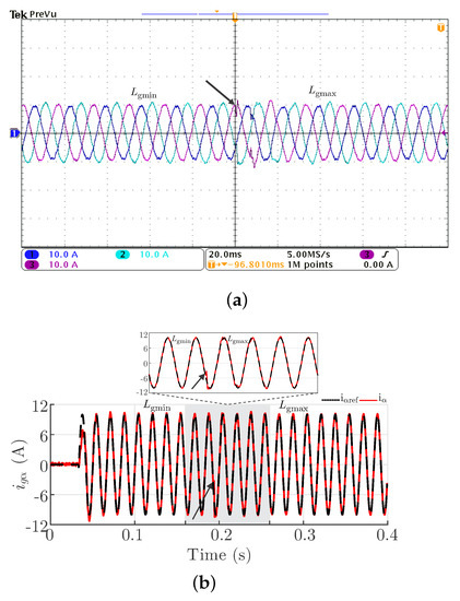
Figure 10. Experimental results for a sudden variation of the output inductance from $L_{gmin}$ to $L_{gmax}$ (a) $abc$ coordinates and (b) $\alpha$ axis.

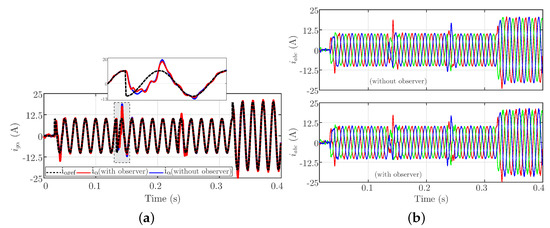
A detailed comparison between the responses of the system operating with the observed states in the control law (i.e., with the observer) and the system operating with the measured state variables (i.e., without the observer) is shown in Figure 11. A good correspondence between the results can be verified, both in transient and steady state, showing that the controller with the proposed robust observer provides responses close to the ones obtained with the measured variables, with the advantage of only requiring the measurement of the grid currents ($i_g$ in $abc$ coordinates).

Figure 11. Experimental result: comparison of the closed-loop system with controller $\mathit{K}\left(Ploc\right)$ in (36), operating with the observed states (observer with gains in (37)) and with real states (i.e., operation with measured states). (a) $\alpha$ axis; (b) $abc$ coordinates.

Notice that the proposed procedure can be used also with different robust controllers, enabling the implementation with a reduced number of sensors. To exemplify that, instead of using step 1 to design the control gains, consider other LMI-based strategies in the literature, such as [22,23,38]. Using these strategies for the parameters in Table 1, one can obtain the control gains given in Table 2 (truncated with 4 decimal digits). Then, following step 2 of the procedure, the parameter $r=0.93$ was chosen, and (27) is used to compute the observer gains, leading to the same gains in (37). The robustness was certified by the step 3, and the LMIs in Appendix B ensure stability for $b=1$, for the closed-loop systems with all these controllers. In other words, in this case study, the use of the observer designed with the proposed procedure, together with any of the control gains in Table 2, leads to stable closed-loop systems for arbitrarily fast time variations of the grid inductance from $L_{gmin}$ to $L_{gmax}$.

Table 2. Robust control gains for a performance comparison.

${\mathit{K}}^{\prime }\left({𝓗}_2\right)$ [23]	${\mathit{K}}^{\prime }\left(\mathit{DLQR}\right)$ [38]	${\mathit{K}}^{\prime }\left({𝓗}_{\mathit{\infty }}\right)$ [22]
−9.6718	−13.7786	−14.1802
−1.8679	−2.9643	−3.2249
0.4376	−2.2487	−1.5748
−0.4417	−0.6212	−0.6369
38.6459	78.9283	23.5127
−38.1467	−77.9606	−23.5994
12.0217	28.7651	23.7455
−11.8015	−28.0124	−24.4868
5.7502	18.6829	25.2601
−5.9453	−18.7725	−27.1579
2.1271	11.4726	30.9341
−2.4812	−12.2583	−33.5741

Figure 12 shows the experimental results for the closed-loop system with four different controllers from the literature. One can confirm from Figure 12a (in $\alpha$ axis) that, despite of different responses for each controller, all the closed-loop systems with feedback of the observed states present suitable time responses. Figure 12b,d,f,h show corresponding experimental results for three-phase grid currents. Figure 12c,e,g,i show experimental results, for a test with sinusoidal references with constant amplitude $(i_{\alpha ref}=20A)$, to verify whether the harmonic spectrum of the grid injected currents in steady state complies with the requirements for individual harmonic components established by IEEE Standard 1547. The total harmonic distortions (THD) are 2.13%, 2.28%, 2.08% and 2.15%, respectively, and all these robust controllers, implemented together with the proposed robust observer, respect the limit of 5% and also the limits of individual harmonics, from this Standard.

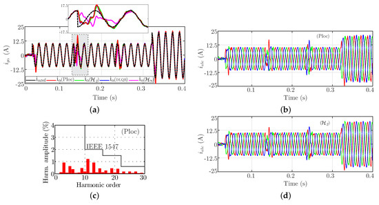
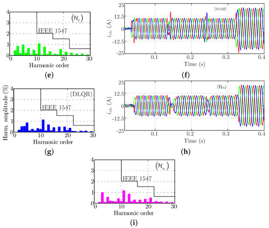
Figure 12. Experimental results for the closed-loop system with the controller $\mathit{K}\left(P_{loc}\right)$ in (36) and the controllers in Table 2, using the observer gains designed with the proposed procedure, in (37). (a) Comparative responses to the $\alpha$ axis. (b–i) Individual responses in $abc$ coordinates and harmonic analysis for the controllers: (b,c) $\mathit{K}\left(P_{loc}\right)$ with THD = 2.13% (d,e) $\mathit{K}\left({\mathcal{H}}_2\right)$ with THD = 2.28% (f,g) $\mathit{K}\left(DLQR\right)$ with THD = 2.08% (h,i) $\mathit{K}\left({\mathcal{H}}_{\infty }\right)$ with THD = 2.15%.

6. Analysis of Guaranteed Stability Regions

The aim of this section is to show that the LMIs in Appendix B can provide less conservative estimations for the regions of guaranteed stability of the closed-loop system, leading to new information with respect to the ones provided by LMIs already explored in the literature for grid-connected converters [20,21,22].

To illustrate this, consider the control and observer gains shown in (36) and (37), designed applying the proposed procedure for the case study. The closed-loop stability with these gains has been certified in the last section, with $b=1$ for $0mH\le L_g\le 1$ mH. On the other hand, now applying the LMIs in Appendix B for progressive increase in the value of $L_{gmax}$, and then computing the maximum value of b for which these LMIs are feasible, it is possible to obtain the region of guaranteed stability shown in Figure 13a.

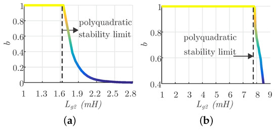
Figure 13. Regions of guaranteed stability provided by the LMIs in the Appendix B: (a) closed-loop system with gains (36) and (37); (b) closed-loop system redesigned for larger grid inductance intervals.

The stability in this case is actually ensured for arbitrarily fast variations of $L_g$ from 0 mH to an $L_{gmax}$ up to $1.65$ mH, which represents a stability region larger then the one addressed in the last section. This conclusion can be confirmed by the LMIs of polyquadratic stability, already explored in the literature for grid-connected converters [20,40]. Nevertheless, the most important outcome here can be seen in the region with $L_{gmax}$ from $1.65$ mH up to $2.8$ mH, where the usual LMIs from the polyquadratic stability do not provide solution, but the LMIs in Appendix B can provide Lyapunov functions for $b<1$, allowing to certify the closed-loop stability by decreasing the bound for the variation rate as $L_{gmax}$ increases. Up to the authors knowledge, the stability domain shown in Figure 13a has not been addressed in the literature with LMIs applied to grid-connected converters, providing new and important information for the control designer.

The LMIs in Appendix B can help to provide even larger estimates of the region of stability. This can be achieved in the case where the control and observer gains are redesigned for larger grid inductance intervals, allowing to encompass from strong to weak grid conditions, for instance. Then, for each new pair of gains $\mathit{K}$ and $\Gamma$, the closed-loop stability can be certified with the LMIs in Appendix B, leading to the region of stability shown in Figure 13b. One can verify that by redesigning the gains, it is possible to ensure stability under arbitrarily fast variations (i.e., $b=1$) for intervals with $L_{gmax}$ up to $7.7$ mH. From this value on, the aforementioned LMIs for polyquadratic stability analysis can no longer certify the stability, but the LMIs in Appendix B can still guarantee stability for $b<1$, that is, for bounded variations of $L_g$. In practical applications, to be able to certify the stability with $b<1$ is an important feature, given that the inductances at the PCC hardly vary instantly from the minimum to the maximum value, especially considering wider ranges.

7. Conclusions

This paper provided a new strategy for the design and implementation of robust current controllers based on state observers for three-phase grid-connected converters with LCL filters. The proposed procedure is based on LMIs that allow obtaining off-line the controller and the observer vector gains in a very fast way, in the scenario of uncertain and possibly time-varying grid impedance parameters. The robust stability of the closed-loop system is ensured by means of less conservative LMIs, based on extra variables, which allow to obtain larger regions of guaranteed stability, which include previous results based on polyquadratic stability. A case study borrowed from the literature is addressed in the paper, because it brings a set of parameters that was used in several papers of robust state feedback control applied to grid connected converters with LCL filters but without using a robust state observer. The control and observer gains designed here ensure good tracking of sinusoidal grid currents. Simulation and experimental results confirm robust performance, as well as compliance with the IEEE 1547 in terms of harmonic content, for the entire range of grid impedances. The proposed procedure allows the implementation of state feedback current controllers with a reduced number of sensors, without significant loss of performance with respect to full measured state vector, being an alternative for robust control based on observed states for grid-connected converters, directly applicable for other filter and grid parameters. Finally, the prospects for future work are inclusion of nonlinearities, such as saturation of actuators, magnetic saturation of LCL filter inductors, in the mathematical model and obtaining robust controllers and observers through LMIs and control of multiple parallel converters, addressing the problems of performance and stability.

References

- Rick, R.; Berton, L. Energy forecasting model based on CNN-LSTM-AE for many time series with unequal lengths. Eng. Appl. Artif. Intell. 2022, 113, 104998. [Google Scholar] [CrossRef]
- Wang, Y.; He, X.; Zhang, L.; Ma, X.; Wu, W.; Nie, R.; Chi, P.; Zhang, Y. A novel fractional time-delayed grey Bernoulli forecasting model and its application for the energy production and consumption prediction. Eng. Appl. Artif. Intell. 2022, 110, 104683. [Google Scholar] [CrossRef]
- Hoffert, M.I.; Caldeira, K.; Benford, G.; Criswell, D.R.; Green, C.; Herzog, H.; Jain, A.K.; Kheshgi, H.S.; Lackner, K.S.; Lewis, J.S.; et al. Advanced technology paths to global climate stability: Energy for a greenhouse planet. Science 2002, 298, 981–987. [Google Scholar] [CrossRef]
- Babatunde, O.M.; Munda, J.L.; Hamam, Y. Power system flexibility: A review. Energy Rep. 2020, 6, 101–106. [Google Scholar] [CrossRef]
- Ram, M.; Child, M.; Aghahosseini, A.; Bogdanov, D.; Lohrmann, A.; Breyer, C. A comparative analysis of electricity generation costs from renewable, fossil fuel and nuclear sources in G20 countries for the period 2015–2030. J. Clean. Prod. 2018, 199, 687–704. [Google Scholar] [CrossRef]
- Akaev, A.A.; Davydova, O.I. A mathematical description of selected energy transition scenarios in the 21st century, intended to realize the main goals of the paris climate agreement. Energies 2021, 14, 2558. [Google Scholar] [CrossRef]
- Chapman, A.J.; McLellan, B.C.; Tezuka, T. Prioritizing mitigation efforts considering co-benefits, equity and energy justice: Fossil fuel to renewable energy transition pathways. Appl. Energy 2018, 219, 187–198. [Google Scholar] [CrossRef]
- Zappa, W.; Junginger, M.; Van Den Broek, M. Is a 100% renewable European power system feasible by 2050? Appl. Energy 2019, 233, 1027–1050. [Google Scholar] [CrossRef]
- Diesendorf, M.; Elliston, B. The feasibility of 100% renewable electricity systems: A response to critics. Renew. Sustain. Energy Rev. 2018, 93, 318–330. [Google Scholar] [CrossRef]
- Nam, K.; Hwangbo, S.; Yoo, C. A deep learning-based forecasting model for renewable energy scenarios to guide sustainable energy policy: A case study of Korea. Renew. Sustain. Energy Rev. 2020, 122, 109725. [Google Scholar] [CrossRef]
- Gidwani, L.; Tiwari, H.; Bansal, R. Improving power quality of wind energy conversion system with unconventional power electronic interface. Int. J. Electr. Power Energy Syst. 2013, 44, 445–453. [Google Scholar] [CrossRef]
- Fuso Nerini, F.; Tomei, J.; To, L.S.; Bisaga, I.; Parikh, P.; Black, M.; Borrion, A.; Spataru, C.; Castán Broto, V.; Anandarajah, G.; et al. Mapping synergies and trade-offs between energy and the Sustainable Development Goals. Nat. Energy 2018, 3, 10–15. [Google Scholar] [CrossRef]
- Chung, H.S.; He, Y.; Huang, M.; Wu, W.; Blaabjerg, F. Robust Hybrid Damper Design for LCL/LLCL-Filtered Grid-Connected Inverter. In Control and Filter Design of Single-Phase Grid-Connected Converters; Wiley Online Library: New York, NY, USA, 2023; pp. 139–162. [Google Scholar] [CrossRef]
- Chen, W.; Zhang, Y.; Tu, Y.; Guan, Y.; Shen, K.; Liu, J. Unified Active Damping Strategy Based on Generalized Virtual Impedance in LCL-Type Grid-Connected Inverter. IEEE Trans. Ind. Electron. 2023, 1–11. [Google Scholar] [CrossRef]
- Cai, Y.; He, Y.; Zhang, H.; Zhou, H.; Liu, J. Integrated Design of Filter and Controller Parameters for Low-Switching-Frequency Grid-Connected Inverter Based on Harmonic State-Space Model. IEEE Trans. Power Electron. 2023, 1–19. [Google Scholar] [CrossRef]
- DeConto, R.M.; Pollard, D.; Alley, R.B.; Velicogna, I.; Gasson, E.; Gomez, N.; Sadai, S.; Condron, A.; Gilford, D.M.; Ashe, E.L.; et al. The Paris Climate Agreement and future sea-level rise from Antarctica. Nature 2021, 593, 83–89. [Google Scholar] [CrossRef]
- Rehman, A.; Rauf, A.; Ahmad, M.; Chandio, A.A.; Deyuan, Z. The effect of carbon dioxide emission and the consumption of electrical energy, fossil fuel energy, and renewable energy, on economic performance: Evidence from Pakistan. Environ. Sci. Pollut. Res. 2019, 26, 21760–21773. [Google Scholar] [CrossRef]
- Boyd, S.; El Ghaoui, L.; Feron, E.; Balakrishnan, V. Linear Matrix Inequalities in System and Control Theory; SIAM Studies in Applied Mathematics: Philadelphia, PA, USA, 1994. [Google Scholar]
- Sturm, J.F. Using SeDuMi 1.02, a MATLAB toolbox for optimization over symmetric cones. Optim. Methods Softw. 1999, 11–12, 625–653. Available online: http://sedumi.mcmaster.ca/ (accessed on 15 February 2023). [CrossRef]
- Maccari, L.A., Jr.; Massing, J.R.; Schuch, L.; Rech, C.; Pinheiro, H.; Oliveira, R.C.L.F.; Montagner, V.F. LMI-Based Control for Grid-Connected Converters With LCL Filters Under Uncertain Parameters. IEEE Trans. Power Electron. 2014, 29, 3776–3785. [Google Scholar] [CrossRef]
- Maccari, L.A., Jr.; Pinheiro, H.; Oliveira, R.C.L.F.; Montagner, V.F. Robust Pole Location with Experimental Validation for Three-Phase Grid-Connected Converters. Control Eng. Pract. 2017, 59, 16–26. [Google Scholar] [CrossRef]
- Koch, G.G.; Maccari, L.A., Jr.; Oliveira, R.C.L.F.; Montagner, V.F. Robust ∞ State Feedback Controllers based on LMIs applied to Grid-Connected Converters. IEEE Trans. Ind. Electron. 2019, 66, 6021–6031. [Google Scholar] [CrossRef]
- Osório, C.R.D.; Koch, G.G.; Oliveira, R.C.L.F.; Montagner, V.F. A practical design procedure for robust 2 controllers applied to grid-connected inverters. Control Eng. Pract. 2019, 92, 104157. [Google Scholar] [CrossRef]
- Luenberger, D.G. Introduction to Dynamic Systems. Theory, Models & Apllications; John Wiley & Sons: New York, NY, USA, 1979. [Google Scholar]
- García, P.; Sumner, M.; Navarro-Rodríguez, Á.; Guerrero, J.M.; García, J. Observer-Based Pulsed Signal Injection for Grid Impedance Estimation in Three-Phase Systems. IEEE Trans. Ind. Electron. 2018, 65, 7888–7899. [Google Scholar] [CrossRef]
- Zhao, J.; Wu, W.; Shuai, Z.; Luo, A.; Chung, H.S.; Blaabjerg, F. Robust Control Parameters Design of PBC Controller for LCL-Filtered Grid-Tied Inverter. IEEE Trans. Power Electron. 2020, 35, 8102–8115. [Google Scholar] [CrossRef]
- Miskovic, V.; Blasko, V.; Jahns, T.; Smith, A.; Romenesko, C. Observer-Based Active Damping of LCL Resonance in Grid-Connected Voltage Source Converters. IEEE Trans. Ind. Appl. 2014, 50, 3977–3985. [Google Scholar] [CrossRef]
- Kukkola, J.; Hinkkanen, M.; Zenger, K. Observer-Based State-Space Current Controller for a Grid Converter Equipped With an LCL Filter: Analytical Method for Direct Discrete-Time Design. IEEE Trans. Ind. Appl. 2015, 51, 4079–4090. [Google Scholar] [CrossRef]
- Rahman, F.M.M.; Riaz, U.; Kukkola, J.; Routimo, M.; Hinkkanen, M. Observer-Based Current Control for Converters with an LCL Filter: Robust Design for Weak Grids. In Proceedings of the 2018 IEEE 9th International Symposium on Sensorless Control for Electrical Drives (SLED), Helsinki, Finland, 13–14 September 2018; pp. 36–41. [Google Scholar] [CrossRef]
- Tang, X.; Chen, W.; Zhang, M. A Current Decoupling Control Scheme for LCL-Type Single-Phase Grid-Connected Converter. IEEE Access 2020, 8, 37756–37765. [Google Scholar] [CrossRef]
- Zhang, H.; Xian, J.; Shi, J.; Wu, S.; Ma, Z. High Performance Decoupling Current Control by Linear Extended State Observer for Three-Phase Grid-Connected Inverter With an LCL Filter. IEEE Access 2020, 8, 13119–13127. [Google Scholar] [CrossRef]
- Su, M.; Cheng, B.; Sun, Y.; Tang, Z.; Guo, B.; Yang, Y.; Blaabjerg, F.; Wang, H. Single-Sensor Control of LCL-Filtered Grid-Connected Inverters. IEEE Access 2019, 7, 38481–38494. [Google Scholar] [CrossRef]
- Zhang, B.; Zhou, X.; Ma, Y. Improved Linear Active Disturbance Rejection Control of Photovoltaic Grid Connected Inverter Based on Filter Function. IEEE Access 2021, 9, 141725–141737. [Google Scholar] [CrossRef]
- Lien, C.H. Robust observer-based control of systems with state perturbations via LMI approach. IEEE Trans. Autom. Control 2004, 49, 1365–1370. [Google Scholar] [CrossRef]
- Kheloufi, H.; Zemouche, A.; Bedouhene, F.; Boutayeb, M. On LMI conditions to design observer-based controllers for linear systems with parameter uncertainties. Automatica 2013, 49, 3700–3704. [Google Scholar] [CrossRef]
- Peaucelle, D.; Ebihara, Y. LMI results for robust control design of observer-based controllers, the discrete-time case with polytopic uncertainties. In Proceedings of the 19th World Congress The International Federation of Automatic Control, Cape Town, South Africa, 24–29 August 2014; pp. 6527–6532. [Google Scholar]
- Koch, G.G.; Maccari, L.A.; Massing, J.R.; Pinheiro, H.; Oliveira, R.C.L.F.; Montagner, V.F. Robust control based on state observer applied to grid-connected converters. In Proceedings of the 2016 12th IEEE International Conference on Industry Applications (INDUSCON), Curitiba, Brazil, 20–23 November 2016; pp. 1–6. [Google Scholar]
- Maccari, L.A.; Santini, C.L.A.; Pinheiro, H.; Oliveira, R.C.L.F.; Montagner, V.F. Robust optimal current control for grid-connected three-phase pulse-width modulated converters. IET Power Electron. 2015, 8, 1490–1499. [Google Scholar] [CrossRef]
- Lee, J.W. On uniform stabilization of discrete-time linear parameter-varying control systems. IEEE Trans. Autom. Control 2006, 51, 1714–1721. [Google Scholar] [CrossRef]
- Daafouz, J.; Bernussou, J. Parameter dependent Lyapunov functions for discrete time systems with time varying parameter uncertainties. Syst. Control Lett. 2001, 43, 355–359. [Google Scholar] [CrossRef]
- Liu, Q.; Caldognetto, T.; Buso, S. Stability Analysis and Auto-Tuning of Interlinking Converters Connected to Weak Grids. IEEE Trans. Power Electron. 2019, 34, 9435–9446. [Google Scholar] [CrossRef]
- Duesterhoeft, W.; Schulz, M.W.; Clarke, E. Determination of Instantaneous Currents and Voltages by Means of Alpha, Beta, and Zero Components. Trans. Am. Inst. Electr. Eng. 1951, 70, 1248–1255. [Google Scholar] [CrossRef]
- Oliveira, R.C.L.F.; Peres, P.L.D. Parameter-dependent LMIs in robust analysis: Characterization of homogeneous polynomially parameter-dependent solutions via LMI relaxations. IEEE Trans. Autom. Control 2007, 52, 1334–1340. [Google Scholar] [CrossRef]
- Labit, Y.; Peaucelle, D.; Henrion, D. SeDuMi interface 1.02: A tool for solving LMI problems with SeDuMi. In Proceedings of the 12th IEEE International Symposium on Computer Aided Control System Design, Glasgow, UK, 20 September 2002; pp. 272–277. [Google Scholar]
- Ogata, K. Discrete-Time Control Systems; Prentice Hall: Upper Saddle River, NJ, USA, 1995. [Google Scholar]
- Chen, C.T. Linear System Theory and Design, 3rd ed.; Oxford University Press: New York, NY, USA, 1999. [Google Scholar]
- Teodorescu, R.; Liserre, M.; Rodríguez, P. Grid Converters for Photovoltaic and Wind Power Systems; John Wiley & Sons: New York, NY, USA, 2011. [Google Scholar]
- Teodorescu, R.; Blaabjerg, F.; Liserre, M.; Loh, P. Proportional-resonant controllers and filters for grid-connected voltage-source converters. IEE Proc. Electr. Power Appl. 2006, 153, 750–762. [Google Scholar] [CrossRef]
- Cardoso, R.; de Camargo, R.F.; Pinheiro, H.; Gründling, H.A. Kalman filter based synchronisation methods. Gener. Transm. Distrib. IET 2008, 2, 542–555. [Google Scholar] [CrossRef]
- Blanchini, F.; Miani, S. Stabilization of LPV Systems: State Feedback, State Estimation, and Duality. SIAM J. Control Optim. 2003, 42, 76–97. [Google Scholar] [CrossRef]
- Bertolin, A.L.J.; Peres, P.L.D.; Oliveira, R.C.L.F. Robust stability,2 and ∞ guaranteed costs for discrete time-varying uncertain linear systems with constrained parameter variations. In Proceedings of the 2019 American Control Conference, Philadelphia, PA, USA, 10–12 July 2019; pp. 4541–4546. [Google Scholar]
- Avis, D.; Fukuda, K. A pivoting algorithm for convex hulls and vertex enumeration of arrangements and polyhedra. Discret. Comput. Geom. 1992, 8, 295–313. [Google Scholar] [CrossRef]
- Herceg, M.; Kvasnica, M.; Jones, C.N.; Morari, M. Multi-Parametric Toolbox 3.0. In Proceedings of the 2013 European Control Conference, Zürich, Switzerland, 17–19 July 2013; pp. 502–510. [Google Scholar]
- de Oliveira, M.C.; Skelton, R.E. Stability tests for constrained linear systems. In Perspectives in Robust Control; Reza Moheimani, S.O., Ed.; Lecture Notes in Control and Information Science; Springer: New York, NY, USA, 2001; Volume 268, pp. 241–257. [Google Scholar]
- Agulhari, C.M.; Felipe, A.; Oliveira, R.C.L.F.; Peres, P.L.D. Algorithm 998: The Robust LMI Parser—A toolbox to construct LMI conditions for uncertain systems. ACM Trans. Math. Softw. 2019, 45, 36. Available online: http://rolmip.github.io (accessed on 15 February 2023). [CrossRef]
Disclaimer/Publisher’s Note: The statements, opinions and data contained in all publications are solely those of the individual author(s) and contributor(s) and not of MDPI and/or the editor(s). MDPI and/or the editor(s) disclaim responsibility for any injury to people or property resulting from any ideas, methods, instructions or products referred to in the content. |
© 2023 by the authors. Licensee MDPI, Basel, Switzerland. This article is an open access article distributed under the terms and conditions of the Creative Commons Attribution (CC BY) license (https://creativecommons.org/licenses/by/4.0/).