Application of Circular Thermoeconomics to the Diagnosis of Energy Systems

Abstract

This paper reviews the fundamentals of the thermoeconomic diagnosis theory. Thermoeconomic diagnosis is one of the main applications of the exergy cost theory used to identify the causes of additional resource consumption of a system due to inefficiencies in its components, published in the late 1990s. Thermoeconomic diagnosis has usually been applied to diagnose power plants with high consumption of fossil fuels and fixed production. However, it does not consider the final production and waste generation variation. In this paper, Circular Thermoeconomics is applied to analyze in depth the effect of malfunctions on additional waste generation and changes in the final output of the system. This new formulation can be applied to polygeneration systems, where there is a simultaneous variation of final products, and to process integration and industrial symbiosis, where a part of the waste generated by a plant could be reused in other processes or plants.

1. Introduction

The circular economy is an intrinsic part of the ecological transition [1,2,3,4]. The recovery of waste to close material cycles is increasingly necessary for managing natural resources. A recovered waste will be competitive if it costs less than the natural resource it replaces. On the other hand, the widespread practice of externalizing waste makes its production costs extremely indeterminate. A rigorous and objective theory, including diagnostics, is therefore needed to solve the problem of evaluating the costs of waste to exploit it both externally (Industrial Symbiosis and Circular Economy) and internally (Process Optimization). However, as systems and production equipment are subject to inevitable deterioration, it is also necessary to evaluate how this degradation affects production costs, both in terms of products and waste. Indeed, diagnosis and sensitivity analysis go hand in hand, and this is the subject of this paper.

Energy systems diagnosis aims to discover and understand signs of malfunction and quantify their effects. There are two main techniques adopted in energy systems [5]:

• Thermomechanical monitoring conditions are usually adopted in power plants to predict failures.
• Thermodynamic monitoring methodologies are mainly suitable for analysing anomalies causing a reduction in system efficiency.

Thermoeconomic diagnosis belongs to the second type of method. However, its objectives are more general and consist of detecting deviations in process efficiency, locating their main causes and quantifying their effects regarding additional fuel consumption.

The foundation of thermoeconomic diagnosis lies in second law analysis, and the objective is to detect efficiency deviations and quantify their cost in terms of additional fuel consumption by comparing two operating conditions: the current operating condition and a reference condition corresponding to the plant operating under design conditions. Efficiency variation of a component can have different causes, either external to the plant (variation of ambient conditions, plant production and fuel quality) or internal, which are the presence of anomalies due to component degradation (malfunctions) and efficiency variations induced by changes in the operating conditions (dysfunctions).

The development of the thermoeconomic diagnosis began in the 1990s [6,7] with the work of the research group at the University of Zaragoza led by Antonio Valero. The mathematical formulation of the fuel impact formula was developed in [8], based on the principle of non-equivalence of the irreversibilities, introduced by Beyer [9]. The most significant efforts have been concentrated on developing procedures for locating anomalies and quantifying their effects, defining concepts such as intrinsic and induced malfunctions, dysfunctions and malfunction costs and their associated calculation procedures [10].

The TADEUS problem [11], an acronym for Thermoeconomic Approach to the Diagnosis in Energy Utility Systems, was a project aimed at integrating various experiences accumulated by several research groups working in thermoeconomic diagnosis. A set of papers was published in 2004 [12,13,14,15,16], showing different approaches, each with particular characteristics that are complementary to each other.

Thermoeconomic diagnosis has been applied mainly to fossil fuel power plants [17,18]. These systems are characterized by having a single primary product, and their production demand is usually fixed, unlike other types of systems such as polygeneration plants, in which there is a simultaneous variation of final products, or industrial parks, in which part of the waste generated by a process can be reused in other processes or plants. Subsequent works have applied this methodology to refrigeration systems [19,20], refrigeration plants and domestic hot water [21]. Other theoretical approaches to thermoeconomic diagnosis have been presented in recent years [22,23,24,25].

However, the original thermoeconomic diagnostic method did not consider either the variation of final products or the additional waste generation. For this reason, it is necessary to include the effects of a process malfunction in the production variation and waste generation.

Circular Thermoeconomics [26] based on exergy cost theory [27] can answer these shortcomings. It allows the accounting of physical or thermodynamic costs, both functional products and waste generated in parallel [28]. It makes it possible to identify which parts of these costs are due to internal irreversibilities and which are due to waste generated or external irreversibilities.

This approach is based on the analysis of production structure [29]. The role of each subsystem (usually corresponding to a thermodynamic process) in its production structure is defined by the resources (fuel) needed to generate the desired product. This product will be input into other system processes or by external consumers. If exergy is taken as a measure, fuel and product are exergy flows, and the ratio of fuel to product represents the exergy efficiency of the process. Circular Thermoeconomics adds a new layer to include the waste process formation cost. If waste leaves the boundaries of a plant, it dissipates into the environment. Still, its formation costs must be accounted for, identifying its origin and internalizing those costs to the processes that have produced it. A part of this waste could be reused in other processes or plants, in which case, the theory allows for calculating its formation costs or will provide an objective cost as a basis for discussion with other plants interested in using it.

The concept of waste [30] has not been sufficiently analyzed in thermoeconomics. By waste, we mean any unwanted material or energy flow—solid, liquid or gaseous—or a heat, noise or any radiating flow. From a thermodynamic point of view, it is simply the external irreversibility that generates entropy outside the system under analysis. Waste is harmful because it still has exergy, and we have to consume it to get rid of it.

Every time we produce, we generate waste. And every product, sooner or later, also becomes waste. This consideration is essential because it allows us to distinguish between waste from production processes and the end-of-use waste of material goods. The former corresponds to the remains of the resources used in the processes; let us call them primary waste because they are produced simultaneously as the products are obtained. The latter corresponds to the degradation or elimination of material goods of an inorganic nature or the discarding of parts of organic substances. Municipalities usually collect this type of waste, and we call it secondary waste. Their treatment, reduction and disposal require more energy, water and raw materials, which constitute the input for their processing. At the same time, new products and tertiary waste are produced, which include their output. Thermoeconomic analysis can, therefore, be applied to them.

Any manufacture of material goods requires exergy resources that are converted into products and waste, both with their exergy. The difference between the exergy of the resources used minus that of the outputs is called internal irreversibility. When waste crosses the boundaries of the productive system, it still has exergy that will irreversibly degrade when released into the environment. It is deferred more or less in time and can potentially damage the biosphere, see [31]. We call this spontaneous process, external irreversibility. Moreover, at its end-of-life, even products behave as waste if they do not become recycled.

As waste is an integral part of production, waste has a cost [32]. These costs are of two types: on the one hand, since they are part of the production process, resources have been consumed to produce them, and on the other hand, to eliminate them, additional resources are required; the latter costs are called abatement costs. Just as the process of product cost formation is evaluated, the process of waste cost formation must also be assessed. Considering that waste has exergy, it is rational to think it could still be used for production.

Unfortunately, we are far from reusing waste for various reasons such as economic interests, lack of regulation, lack of technologies, lack of knowledge about nature’s mechanisms, and even thermodynamic limitations. Cost externalization is the endorsement of the harm we cause outside the production system. At best, we pay taxes or fines for society to mitigate them or send them to countries that accept them in return for payment. A responsible society should internalize waste and its costs as much as possible.

Thermoeconomics enables attaining a coherent and significant set of costs in a given energy structure. Costing allocation essentially looks for the resources needed to produce both intermediate and final products. Circular Thermoeconomics introduces a general formula of irreversibility costs that connects the second law (internal and external irreversibilities) with the physical costs derived from defining the productive purpose of the plant components. In other words, the conceptual rigour of thermodynamics was provided to the costs of standard economics. See Equations (A26) and (A27) in Appendix B.

The process of waste cost formation is a priority objective in Circular Thermoeconomics. Waste costs must be rigorously assessed, identifying the processes that generated it because they are the compass for decisions to improve production processes, both within production plants and/or in increasingly complex industrial chains. When we internalize waste costs, Equation (A27) will also be accountable for these wastes as (external) irreversibilities. Therefore, if external irreversibilities (wastes) are recovered, the production costs are reduced. The keyword recycling [33] must intrinsically relate to efficiency and cost. It can be used interchangeably by thermoeconomics, circular economy and industrial symbiosis [34,35,36].

In summary, this paper aims to update the thermoeconomic diagnosis theory, including the ideas of Circular Thermoeconomics, to analyze the effects of malfunctions in the additional waste generation and product variation. Therefore, it could be applied to a wide range of energy systems.

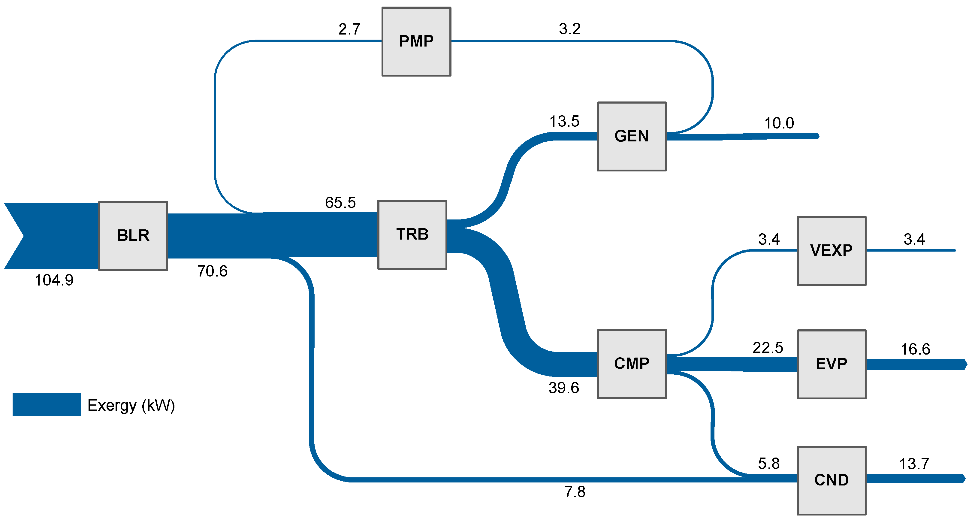
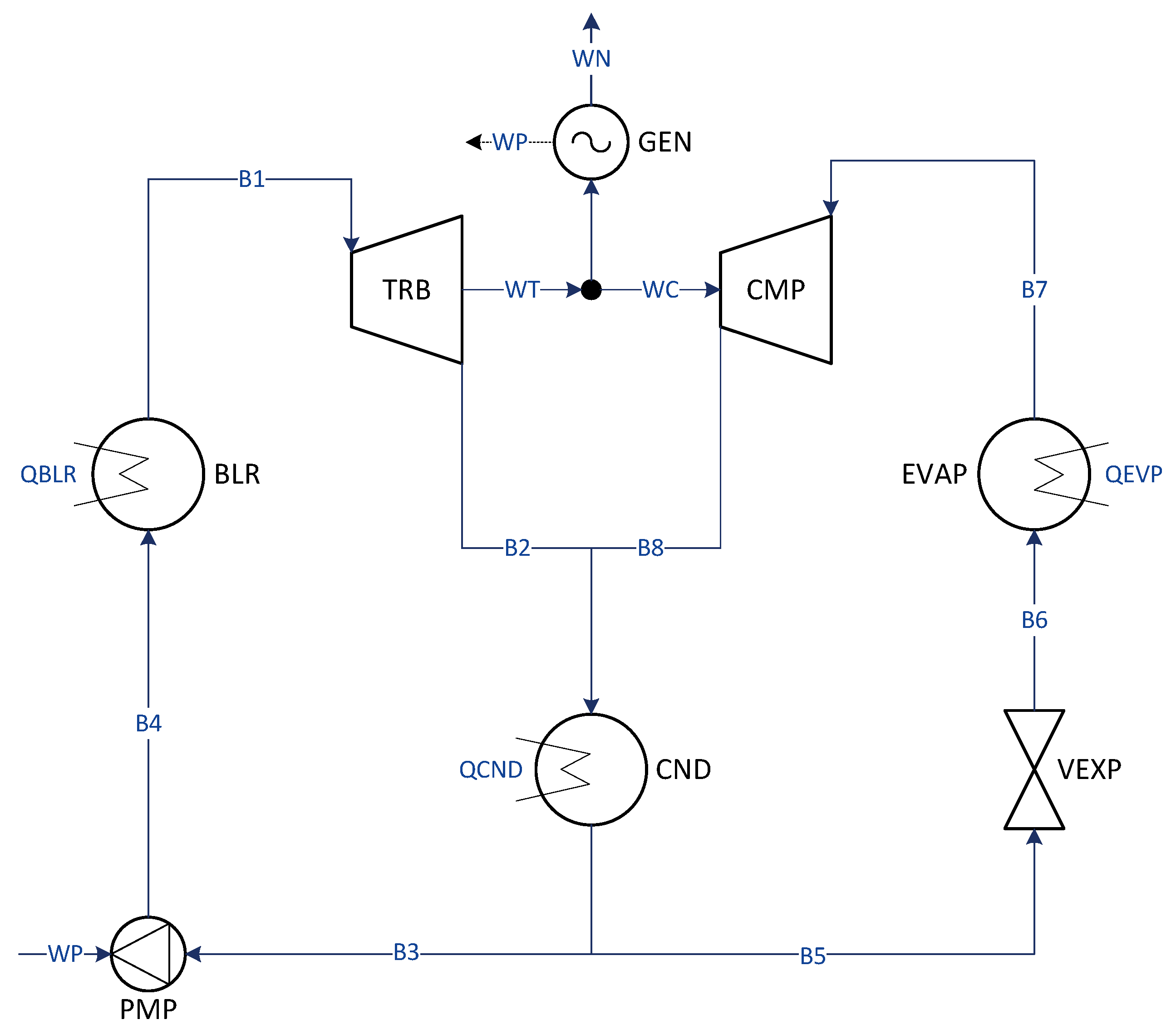
To illustrate the methodology introduced in this paper, an ORC-VCR system to produce electricity and cold is used. The physical and thermoeconomic model of the system is described in Appendix A.

2. Thermoeconomic Diagnosis Fundamentals

This section will briefly review the main concepts of thermoeconomic diagnosis. See also Appendix B for Circular Thermoeconomics nomenclature.

2.1. Technical Exergy Saving

The exergy balance of an installation allows us to allocate and calculate irreversibilities in the production process and to identify the equipment that affects the overall efficiency and the reasons thereof. This information, although helpful, has proved not to be enough. When attempting to achieve energy savings in an installation, we must consider that not all irreversibilities can be avoided. Technical and economic constraints limit the potential exergy saving. Thus, the possibilities for exergy savings, called technical exergy saving, are always lower than the theoretical limit of thermodynamic exergy losses.

Therefore, the additional fuel consumption can be expressed as the plant’s resource consumption difference between operation and reference or design conditions.

$$\Delta F_T=F_T\left(x\right)-F_T\left(x^0\right)$$

(1)

It can be broken up into the sum of the irreversibilities of each component:

$$\Delta F_T=\Delta I_T+\Delta P_T=\sum _{j=1}^n\left(I_j\left(x\right)-I_j\left(x^0\right)\right)=\sum _{j=1}^n\Delta I_j+\sum _{j=1}^n\Delta {\omega }_{0,i}$$

where ${\omega }_{0,i}$ is the exergy of the flows i leaving the plant. In our example, cold and electricity are the final products, but the heat waste rejected in the condenser and the mechanical dissipation in the expansion valve are also system outputs. In matrix notation, it is written as:

$$\Delta F_T={}^{\mathbf{t}}\mathbf{u}\Delta \mathbf{I}+{}^{\mathbf{t}}\mathbf{u}\Delta {\mathit{\omega }}_0$$

(2)

2.2. Malfunction and Dysfunction

Using a thermodynamic model simulator or a plant performance test, we can obtain their exergy flow values and the efficiency of each process. From these operation data, unit exergy consumption and other thermoeconomic variables can be calculated for the operating conditions. These values can be compared concerning those corresponding to the design values of the plant. Usually in operation, several plant components suffer a degradation of their behaviour concerning the design conditions and, as a consequence, their unit exergy consumption increases:

$$\Delta {\kappa }_{ij}={\kappa }_{ij}\left(x\right)-{\kappa }_{ij}\left(x^0\right)\mathrm{and}\Delta k_i=\sum _{j=0}^n\Delta {\kappa }_{ji}$$

(3)

The irreversibility increase in a system’s component, see Appendix A, is given by:

$$\Delta \mathbf{I}=\Delta {\mathbf{K}}_{\mathrm{D}}{\mathbf{P}}^0+\left({\mathbf{K}}_{\mathrm{D}}-{\mathbf{U}}_{\mathrm{D}}\right)\Delta \mathbf{P}$$

(4)

where ${\mathbf{P}}^0\equiv \mathbf{P}\left(x^0\right)$ is the production in the reference conditions, and K_D is a diagonal matrix containing the unit consumption of each process. From the above expression, we can distinguish two types of irreversibilities:

 

Malfunction: is the irreversibility produced by an increase in the unit consumption of the component itself or endogenous irreversibility:

$$\mathbf{M}\mathbf{F}=\Delta {\mathbf{K}}_{\mathrm{D}}{\mathbf{P}}^0$$

(5)

 

where MF is an $(m\times 1)$ vector whose elements contain the malfunction or the variation of the local consumption of the process $M{F}_i\equiv P_i\left(x_0\right)\Delta k_i$.

 

Let $[\mathbf{M}\mathbf{F}]\equiv \Delta ⟨\mathbf{K}\mathbf{P}⟩{\hat{\mathbf{P}}}^0$ be an $(n\times n)$ matrix called local malfunction matrix, where its elements are defined as $M{F}_{ji}=\Delta {\kappa }_{ji}{P}_i\left(x_0\right)$, and represent the increase in each local fuel consumption of process i provided by process j, and let ${\mathbf{M}\mathbf{F}}_0$ to be a $(n\times 1)$ vector, whose elements $M{F}_{0j}=\Delta {\kappa }_{0j}{P}_i\left(x^0\right)$ accounts for the increase in external fuel entering a component, therefore:

$${}^{\mathbf{t}}\mathbf{M}\mathbf{F}={{}^{\mathbf{t}}\mathbf{M}\mathbf{F}}_0+{}^{\mathbf{t}}\mathbf{u}[\mathbf{M}\mathbf{F}]$$

(6)

 

Dysfunction: is the exogenous irreversibility induced in a component by the malfunction of other subsystems, which forces it to consume more local resources to obtain the additional production required by the other components:

$$\mathbf{D}\mathbf{F}=\left({\mathbf{K}}_{\mathrm{D}}-{\mathbf{U}}_{\mathrm{D}}\right)\Delta \mathbf{P}$$

(7)

The degradation of a component forces the other components to adapt their behaviour to maintain their production conditions; consequently, their irreversibilities are modified. Figure 1 shows how an increase in the unit consumption of a component increases not only the irreversibilities of such component but also the irreversibilities of the previous component.

Figure 1. Effect of a local malfunction in a generic system.

To relate the internal irreversibility increase with the variation of local consumption of processes, the production variation due to a local consumption change, see Appendix C, could be written as:

$$\Delta \mathbf{P}=|\mathbf{P}⟩⟨\mathbf{K}\mathbf{P}⟩{\mathbf{P}}^{\left(0\right)}$$

(8)

where |P⟩ is the production matrix in actual operating conditions and ${|\mathbf{P}⟩}^{\left(0\right)}$ is that in reference conditions. Substituting Equation (8) into Equation (7) yields the dysfunctions generated in each component in terms of the unit consumption increment:

$$\mathbf{D}\mathbf{F}=|\mathbf{I}⟩\left(\Delta ⟨\mathbf{K}\mathbf{P}⟩{\mathbf{P}}^0+\Delta {\mathit{\omega }}_0\right)$$

(9)

Let $[\mathbf{D}\mathbf{F}]\equiv |\mathbf{I}⟩[\mathbf{M}\mathbf{F}]$ be an $(n\times n)$ matrix, called dysfunction matrix, whose elements $D{F}_{ij}$ represent the increase in the irreversibility of a process i due to a malfunction of a process j.

Similarly, let ${\mathbf{D}\mathbf{F}}_0\equiv |\mathbf{I}⟩\Delta {\mathit{\omega }}_0$ be an $(n\times 1)$ vector, whose elements are the dysfunctions caused by the increase in the system outputs, both final products and wastes. Hence, the vector $\Delta \mathbf{I}$, which contains the increased exergy losses of each process, is written as:

$$\Delta \mathbf{I}=\mathbf{M}\mathbf{F}+[\mathbf{D}\mathbf{F}]\mathbf{u}+{\mathbf{D}\mathbf{F}}_0$$

(10)

It means that the irreversibility increase of a process is due to its local malfunctions plus all the dysfunctions caused by interactions with the rest of the system processes and the dysfunction produced by the system outputs (both products and waste) variation.

Figure 2 shows the causes of irreversibilities due to malfunction in the turbine (MF bar). This malfunction causes a decrease in the cold production equal to the sum of irreversibilities (internal and external). The malfunction increases the irreversibility of the turbine and creates a dysfunction in the boiler (BLR blue bar). Note the influence of the production variation (ENV orange bar) and waste variation (VEXP, CND bars) on the irreversibilities of the processes. Equation (10) locates the effect of malfunction in the variation of the local irreversibilities of the plant components but not the causes of waste variation. This effect is analyzed in detail in the next section.

Figure 2. Irreversibility variation graph for the TCND35 simulation, according to Equation (10).

2.3. Malfunction Cost and Fuel Impact Fuel

The total fuel consumption of a system, see Equation (A25) in Appendix B, is written as:

$$F_T={{}^{\mathbf{t}}\mathit{\kappa }}_e\mathbf{P}={{}^{\mathbf{t}}\mathit{\kappa }}_e|\mathbf{P}⟩{\mathit{\omega }}_0={}^{\mathbf{t}}\mathbf{k}_P^{\mathit{in}}{\mathit{\omega }}_0$$

(11)

In these equations, the total fuel is only a function of the local unit consumption and the system outputs, including waste. Applying matrix difference calculus, see Appendix C, the fuel impact could be expressed as:

$$\Delta F_T=\left(\Delta {{}^{\mathbf{t}}\mathit{\kappa }}_e+{}^{\mathbf{t}}\mathbf{k}_P^{\mathit{in}}\Delta ⟨\mathbf{K}\mathbf{P}⟩\right){\mathbf{P}}^0+{}^{\mathbf{t}}\mathbf{k}_P^{\mathit{in}}\Delta {\mathit{\omega }}_0$$

(12)

and applying the malfunction definition:

$$\Delta F_T={}^{\mathbf{t}}\mathbf{u}_n{\mathbf{M}\mathbf{F}}_0+{}^{\mathbf{t}}\mathbf{k}_P^{\mathit{in}}[\mathbf{M}\mathbf{F}]\mathbf{u}+{}^{\mathbf{t}}\mathbf{k}_P^{\mathit{in}}\Delta {\mathit{\omega }}_0$$

(13)

This expression is called Fuel Impact Formula. It expresses resource consumption’s variation as a function of the local consumption variation $\Delta {\kappa }_{ij}$ and the variation of system outputs 0 evaluated at the production cost due only to internal irreversibilities.

Let us define the malfunction cost as the effect of a local malfunction on resource consumption.

$${{}^{\mathbf{t}}\mathbf{M}\mathbf{F}}^{*}\equiv {{}^{\mathbf{t}}\mathbf{M}\mathbf{F}}_0+{}^{\mathbf{t}}\mathbf{k}_P^{\mathit{in}}[\mathbf{M}\mathbf{F}],$$

(14)

and the fuel impact is written in terms of malfunction costs as:

$$\Delta F_T={}^{\mathbf{t}}\mathbf{u}_n{\mathbf{M}\mathbf{F}}^{*}+{}^{\mathbf{t}}\mathbf{k}_P^{\mathit{in}}\Delta {\mathit{\omega }}_0$$

(15)

On the other hand, applying Equation (A26) to the malfunction cost definition:

$${{}^{\mathbf{t}}\mathbf{M}\mathbf{F}}^{*}={{}^{\mathbf{t}}\mathbf{M}\mathbf{F}}_0+{}^{\mathbf{t}}\mathbf{u}_n({\mathbf{U}}_{\mathrm{D}}+|\mathbf{I}⟩)[\mathbf{M}\mathbf{F}]$$

therefore:

$${{}^{\mathbf{t}}\mathbf{M}\mathbf{F}}^{*}={}^{\mathbf{t}}\mathbf{M}\mathbf{F}+{}^{\mathbf{t}}\mathbf{u}_n[\mathbf{D}\mathbf{F}]$$

(16)

It means that the malfunction cost of a process accounts for its malfunction process plus all the dysfunction generated in the rest of the processes.

Note that, in Equation (13), the fuel impact of a malfunction in process $-i-$ is quantified by the unit cost of the product of process $-j-$, used as fuel for process $-i-$. This cost only includes the effect of internal irreversibilities. This unit cost also quantifies the output variation, but this variation in output includes both the final products and the waste generated. Both affect the impact on fuel but in very different ways. In the case of waste, an increase means an irreversible loss of resources, while in the case of a final product variation, the conclusion is very different. If production decreases, the impact on fuel also decreases, but at the cost of reducing profits and increasing the amortization time of the system. If production increases, the situation is just the opposite. Therefore, the fuel impact formula Equation (15) for plant diagnosis is insufficient when the total production is not constant. These facts will be analyzed in depth in the next section.

3. The Effect of Malfunctions in Waste Generation

This section will analyze the impact of malfunction on the increasing waste generation. First, we will obtain a formula that relates the component’s malfunction with the variation of the generated waste. The variation of the system’s outputs can be split as:

$$\Delta {\mathit{\omega }}_0=\Delta {\mathit{\omega }}_t+\Delta {\mathit{\omega }}_r$$

where Δω_t is the variation of the final production and Δω_r is the variation of waste generated. On the other hand, according to Equation (A14), the waste generation could be written as: ${\mathit{\omega }}_r=⟨\mathbf{K}\mathbf{R}⟩\mathbf{P}$.

First, applying matrix difference calculus, we obtain an expression relating the variation of the waste exergy to the internal malfunctions of the processes:

$$\Delta {\mathit{\omega }}_r=|\tilde{\mathbf{R}}⟩\Delta ⟨\mathbf{K}\mathbf{P}⟩{\mathbf{P}}^0+\left({\mathbf{U}}_{\mathrm{D}}+|\tilde{\mathbf{R}}⟩\right)\Delta ⟨\mathbf{K}\mathbf{R}⟩{\mathbf{P}}^0+|\tilde{\mathbf{R}}⟩\Delta {\mathit{\omega }}_t$$

(17)

The first and second terms of Equation (17) show the effect of internal malfunctions $\Delta ⟨\mathbf{K}\mathbf{P}⟩{\mathbf{P}}^0$ and the variation of waste allocation ratios $\Delta ⟨\mathbf{K}\mathbf{P}⟩{\mathbf{P}}^0$. The last term is the effect of the variation of final products. Then, the fuel impact due to waste variation could be written as:

$${}^{\mathbf{t}}\mathbf{k}_P^{\mathit{in}}\Delta {\mathit{\omega }}_r={}^{\mathbf{t}}\mathbf{k}_P^{\mathit{ex}}\Delta ⟨\mathbf{K}\mathbf{P}⟩{\mathbf{P}}^0+{}^{\mathbf{t}}\mathbf{k}_P^{*}\Delta ⟨\mathbf{K}\mathbf{P}⟩{\mathbf{P}}^0+{}^{\mathbf{t}}\mathbf{k}_P^{\mathit{ex}}\Delta {\mathit{\omega }}_t$$

(18)

Let us define the waste cost impact as the effect of the waste variation on the resource consumption:

$${{}^{\mathbf{t}}\mathbf{M}\mathbf{R}}^{*}\equiv {}^{\mathbf{t}}\mathbf{k}_P^{\mathit{ex}}[\mathbf{M}\mathbf{F}]+{}^{\mathbf{t}}\mathbf{k}_P^{*}[\mathbf{M}\mathbf{R}]$$

(19)

where $[\mathbf{M}\mathbf{R}]\equiv \Delta ⟨\mathbf{K}\mathbf{R}⟩{\hat{\mathbf{P}}}^0$ is the equivalent malfunction matrix to the waste generation ratios. Note that these ratios implicitly depend on the unit consumption of the processes and, hence, on the internal dysfunctions.

Therefore, the fuel impact formula Equation (15) could be rewritten as:

$$\Delta F_T={}^{\mathbf{t}}\mathbf{u}_n{\mathbf{M}\mathbf{F}}^{*}+{}^{\mathbf{t}}\mathbf{u}_n{\mathbf{M}\mathbf{R}}^{*}+{}^{\mathbf{t}}\mathbf{k}_P^{*}\Delta {\mathit{\omega }}_t$$

(20)

Equation (20) shows that the fuel impact is the sum of the malfunction cost, the internal cost of waste variation and the cost of final production changes. The effects of changes in the final system product are assessed with the unit production cost that includes both internal and external irreversibilities. This equation improves Equation (15) and makes it possible to better explain the causes of the variation in resource consumption by separating it into parts due to internal malfunctions, waste malfunctions and production variation.

On the other hand, applying Equation (17) into irreversibility variation Equation (10), we obtain:

$$\Delta \mathbf{I}=\mathbf{M}\mathbf{F}+|\tilde{\mathbf{I}}⟩\left([\mathbf{M}\mathbf{F}]+[\mathbf{M}\mathbf{R}]\right)\mathbf{u}+|\tilde{\mathbf{I}}⟩\Delta {\mathit{\omega }}_t$$

(21)

Equation (21) decomposes the irreversibility variation of each component into the part due to malfunction, the dysfunction caused by internal and external irreversibilities, and the dysfunction due to the variation of demand production.

The fuel impact Equation (13) could be rewritten using Equation (A27) as:

$$\Delta F_T={}^{\mathbf{t}}\mathbf{u}_n{\mathbf{M}\mathbf{F}}_0+{}^{\mathbf{t}}\mathbf{k}_P^{*}[\mathbf{M}\mathbf{F}]\mathbf{u}+{}^{\mathbf{t}}\mathbf{k}_P^{*}[\mathbf{M}\mathbf{R}]\mathbf{u}+{}^{\mathbf{t}}\mathbf{k}_P^{*}\Delta {\mathit{\omega }}_t$$

(22)

This version of the fuel impact formula was first introduced in [37]. Although this form correctly evaluates the cost of variation of final products and considers the impact of waste, it does not allow for the separation of the effects of internal irreversibilities from external ones, as Equation (19) does.

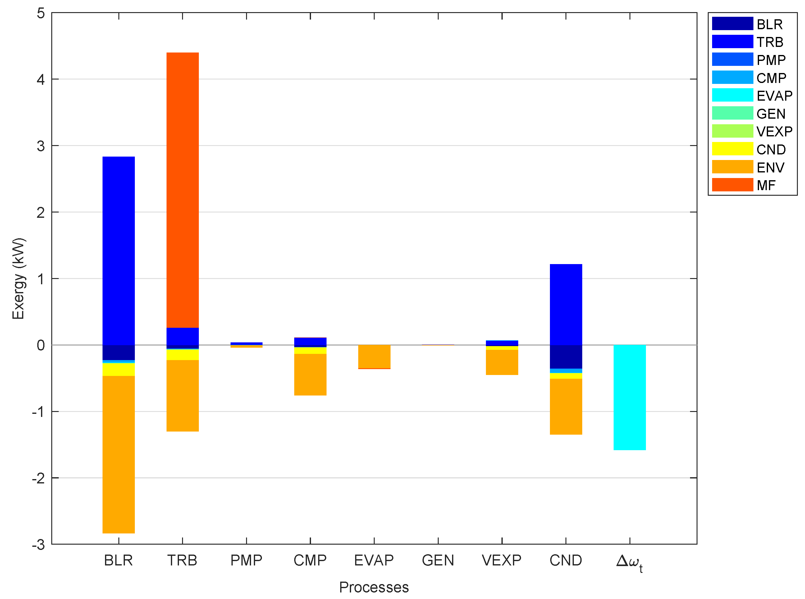
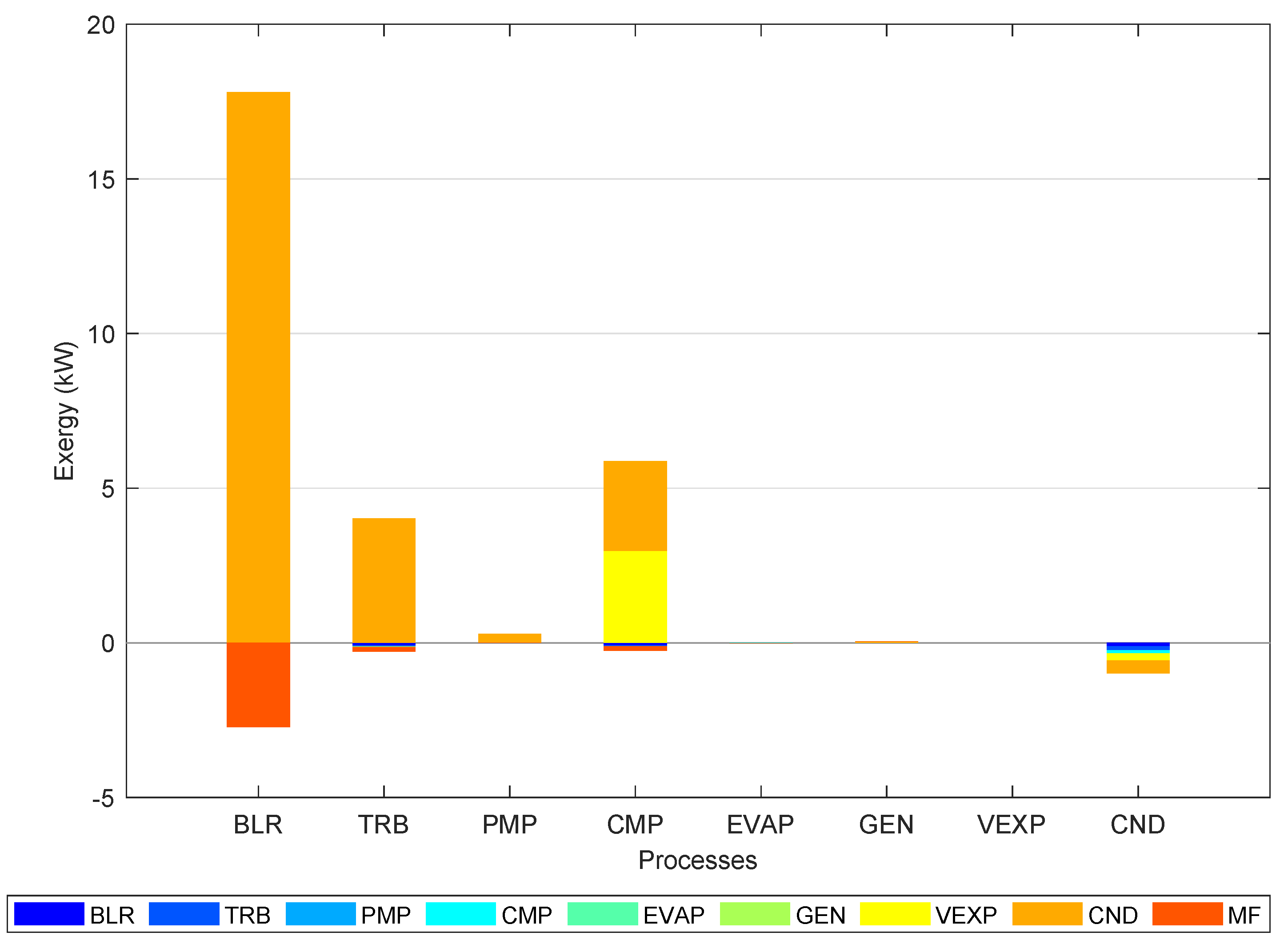
Figure 3 shows the irreversibility variation plot for the TCND35 simulation, using Equation (21). In contrast to Figure 2, this graph identifies the components causing the increase in residuals. The CND column shows that the causes of dissipated waste heat (external irreversibility) are mainly due to the evaporation process (BLR). The dysfunctions of the dissipative components are now replaced by the dysfunctions caused by the production processes that generate the waste. It also illustrates how the decrease in production causes a decrease in irreversibility in the remaining components.

Figure 3. Irreversibility variation graph for the TCND35 simulation, according to Equation (21).

4. Total Malfunction Cost Rate

As explained above, the production variation’s effect on resource consumption must be considered. If production decreases, resource consumption decreases, and vice versa, which could cause some misunderstandings. From Equation (20), we can construct a new indicator to assess the actual resource consumption that considers this issue. We propose the effective fuel impact or total malfunction cost rate defined as follows:

$${\mathcal{M}}_T=\Delta F_T-\Delta {\omega }_t^{*}$$

(23)

where $\Delta {\omega }_t^{*}$ is the effective cost variation of the final product, defined as follows:

$$\Delta {\omega }_t^{*}=\left\{\begin{array}{cc}{}^{\mathbf{t}}\mathbf{k}_P^{*}\left(x_0\right)\Delta {\mathit{\omega }}_t\hfill & \Delta {\mathit{\omega }}_t>0\hfill \\ {}^{\mathbf{t}}\mathbf{k}_P^{*}\left(x\right)\Delta {\mathit{\omega }}_t\hfill & \Delta {\mathit{\omega }}_t<0\hfill \end{array}\right.$$

(24)

The effective cost of the change in production depends on whether the final production increases, in which case it is valued at the reference cost of production, and if output decreases, it is valued at the current production cost.

The total malfunction cost rate could also be expressed as:

$${\mathcal{M}}_T=\left\{\begin{array}{cc}{}^{\mathbf{t}}\mathbf{u}_n{\mathbf{M}\mathbf{F}}^{*}+{}^{\mathbf{t}}\mathbf{u}_n{\mathbf{M}\mathbf{R}}^{*}+\Delta {}^{\mathbf{t}}\mathbf{k}_P^{*}\Delta {\mathit{\omega }}_t\hfill & \Delta {\mathit{\omega }}_t>0\hfill \\ {}^{\mathbf{t}}\mathbf{u}_n{\mathbf{M}\mathbf{F}}^{*}+{}^{\mathbf{t}}\mathbf{u}_n{\mathbf{M}\mathbf{R}}^{*}\hfill & \Delta {\mathit{\omega }}_t<0\hfill \end{array}\right.$$

(25)

It means that the effective fuel impact is the sum of internal and external malfunction costs plus a correction depending on the unit production cost of the final products. Thus, the impact on fuel oil does not depend on variations in production but on malfunctions and the increased irreversibility they cause in other processes, i.e., the cost of malfunctions.

Note that if the resource consumption is constant, a decrease/increase in production causes an increase/decrease in the total irreversibility (internal and external). Similarly, a decrease/increase in production causes an increase/decrease in the cost of internal and external malfunctions.

5. Results

The proposed methodology for thermoeconomic diagnosis will be illustrated in this section with the example shown in Figure A1. This section’s result tables and graphs have been obtained using the software tool TaesLab; see reference [38]. This software implements both sets of algorithms described in the paper: the original diagnosis approach, waste external, which considers waste as external outputs, and the new approach, waste internal, which internalizes the waste costs. We will analyze below the different malfunction simulations described in Table A2, which are also used for sensitivity analysis.

5.1. Case 1: ETAT75

The first simulation analyzes a case of turbine failure, keeping the net power constant, which causes a decrease in the isentropic efficiency of 5%.

The summary of thermoeconomic diagnosis is shown in Table 1. The first column $MF$ shows the malfunction of each component according to Equation (6). The second column $\Delta I$ presents the irreversibility (both internal and external) variation of each process, and the third column $\Delta {\omega }_t$ the final product variation. The total sum of both columns gives the fuel impact. The following two columns provide the malfunction cost $M{F}^{*}$ according to Equation (14) and the waste malfunction cost $M{R}^{*}$. The total sum of both columns gives the effective fuel impact (in case of production decrease). The last column shows the effective cost of the production change, Equation (24).

Table 1. Diagnosis analysis for the ETAT75 simulation (kW).

Key	$\mathit{M}\mathit{F}$	$\mathbf{\Delta }\mathit{I}$	$\mathbf{\Delta }{\mathit{\omega }}_{\mathit{t}}$	${\mathit{M}\mathit{F}}^{*}$	${\mathit{M}\mathit{R}}^{*}$	$\mathbf{\Delta }{\mathit{\omega }}_{\mathit{t}}^{*}$
BLR	0.000	0.000	0.000	0.000	-0.699	0.000
TRB	4.140	3.100	0.000	6.288	2.379	0.000
PMP	0.000	0.000	0.000	0.000	−0.009	0.000
CMP	0.000	−0.651	0.000	0.000	−0.105	0.000
EVAP	−0.008	−0.359	−1.580	−0.020	−0.010	−7.231
GEN	0.000	0.000	0.000	0.000	−0.001	0.000
VEXP	0.000	−0.380	0.000	0.000	0.000	0.000
CND	0.000	−0.130	0.000	−0.297	−0.294	0.000
Total	4.132	1.580	−1.580	5.971	1.260	−7.231

The system’s fuel consumption does not change, but the exergy of the cold production decreases by 1.58 kW, resulting in an increase in irreversibility by the same amount. The turbine malfunction has a value of 4.14 kW (marked in bold in Table 1), and its cost makes the additional resources consumed 7.23 kW. This new methodology lets us identify that 5.97 kW are caused by internal malfunctions (TRB) and 2.38 kW are caused by waste cost variation.

Figure 4 represents the malfunction costs of the simulation and clearly shows that the cause of the actual fuel impact is located in the turbine. The malfunction caused an increase of 2.29 kW in waste heat dissipated from the condenser and an increase in boiler irreversibility of 2 kW.

Figure 4. Malfunction cost graph for the ETAT75 simulation.

5.2. Case 2: ETAC75

This simulation analyzes the effect of a 2% loss in the isentropic efficiency of the compressor, keeping the cold production constant.

In this case, the fuel consumption of the installation does not change, but the net power decreases by 1 kW and the irreversibility of the compressor increases by the same amount. This malfunction increases condenser waste heat by 0.75 kW, and the effective fuel impact is 2.387 kW. The cost due to internal malfunctions is 1.86 kW, and the cost of waste variation is 0.53 kW. See Table 2.

Table 2. Diagnosis analysis for the ETAC78 simulation (kW).

Key	$\mathit{M}\mathit{F}$	$\mathbf{\Delta }\mathit{I}$	$\mathbf{\Delta }{\mathit{\omega }}_{\mathit{t}}$	${\mathit{M}\mathit{F}}^{*}$	${\mathit{M}\mathit{R}}^{*}$	$\mathbf{\Delta }{\mathit{\omega }}_{\mathit{t}}^{*}$
BLR	0.000	0.000	0.000	0.000	−0.271	0.000
TRB	0.000	0.000	0.000	0.000	0.007	0.000
PMP	0.000	0.000	0.000	0.000	−0.004	0.000
CMP	0.982	0.990	0.000	1.835	0.775	0.000
EVAP	0.000	0.000	0.000	0.000	0.000	0.000
GEN	0.000	−0.020	−1.000	0.000	0.003	−2.387
VEXP	0.005	0.010	0.000	0.012	0.006	0.000
CND	0.000	0.020	0.000	0.011	0.012	0.000
Total	0.987	1.000	−1.000	1.859	0.528	−2.387

In Figure 5, it is shown how the cost of the malfunction is located in the compressor and, in particular, in its intrinsic malfunction (1 kW), which in turn causes an increase of the irreversibility in the rest of the components.

Figure 5. Malfunction cost graph for the ETAC78 simulation.

5.3. Case 3: TCND35

This simulation analyzes the effect of a 5 °C increase in condenser temperature, reducing the net power by 1 kW.

In this case, the fuel impact is negative (–3.3 kW), and the cold production is 25% lower. Internal irreversibilities reduce by 6.29 kW, but waste generation increases by 8.56 kW, see Table 3. The internal irreversibilities and their cost are negative. Still, the impact of waste increasing is much larger, 27.395, where the decrease in production represents 27 kW of resources, and the effective fuel impact is 23.793 kW.

Table 3. Diagnosis analysis for the TCND35 simulation (kW).

Key	$\mathit{M}\mathit{F}$	$\mathbf{\Delta }\mathit{I}$	$\mathbf{\Delta }{\mathit{\omega }}_{\mathit{t}}$	${\mathit{M}\mathit{F}}^{*}$	${\mathit{M}\mathit{R}}^{*}$	$\mathbf{\Delta }{\mathit{\omega }}_{\mathit{t}}^{*}$
BLR	−2.721	−2.900	0.000	−2.721	17.811	0.000
TRB	−0.152	−1.400	0.000	−0.276	4.018	0.000
PMP	−0.001	−0.018	0.000	−0.002	0.288	0.000
CMP	−0.141	−0.931	0.000	−0.256	5.878	0.000
EVAP	−0.003	−1.019	−4.570	−0.006	−0.006	−24.272
GEN	0.001	−0.022	−1.000	0.001	0.046	−2.821
VEXP	0.000	0.140	0.000	0.000	0.000	0.000
CND	0.000	8.420	0.000	−0.342	−0.640	0.000
Total	−3.017	2.270	−5.570	−3.602	27.395	−27.093

Figure 6 shows the malfunction cost of each component of the plant. In the case of the boiler, it has a negative malfunction due to the inlet temperature increasing when the condenser temperature increases. Moreover, the boiler is the cause of increasing condenser waste heat of 17.81 kW. In the case of the compressor, it also caused an increase in expansion valve mechanical dissipation by 2.98 kW. It clearly shows that waste malfunction cost is located in the processes that generated the waste; see Table A4.

Figure 6. Malfunction cost graph for the TCND35 simulation.

5.4. Case 4: TBLR85

This simulation analyzes a decrease in the evaporating pressure in the boiler of 1.5 bar, keeping the net power constant and decreasing the cold production by 10%.

In this case, the total fuel consumption of the system decreased by 6.07 kW and the cooling production in terms of exergy by 1.56 kW, so the total irreversibility decreased by 4.51 kW. But on the other hand, boiler and turbine malfunctions increased by 0.384 kW. Therefore, the total malfunction cost or effective fuel impact is favourable at 0.655 kW. See Table 4.

Table 4. Diagnosis analysis for the TBLR85 simulation (kW).

Key	$\mathit{M}\mathit{F}$	$\mathbf{\Delta }\mathit{I}$	$\mathbf{\Delta }{\mathit{\omega }}_{\mathit{t}}$	${\mathit{M}\mathit{F}}^{*}$	${\mathit{M}\mathit{R}}^{*}$	$\mathbf{\Delta }{\mathit{\omega }}_{\mathit{t}}^{*}$
BLR	0.259	−1.820	0.000	0.259	0.642	0.000
TRB	0.127	−0.750	0.000	0.064	−0.015	0.000
PMP	0.011	−0.050	0.000	0.020	0.018	0.000
CMP	0.003	−0.641	0.000	0.006	0.036	0.000
EVAP	−0.013	−0.359	−1.560	−0.030	−0.015	−6.725
GEN	−0.002	−0.010	0.000	−0.004	−0.004	0.000
VEXP	0.000	−0.380	0.000	0.000	0.000	0.000
CND	0.000	−0.500	0.000	−0.159	−0.161	0.000
Total	0.384	−4.510	−1.560	0.156	0.499	−6.725

Figure 7 shows how the boiler malfunction also causes an increase in condenser waste heat. The sum of all positive and negative contributions gives the actual fuel impact. A decrease in production reduces irreversibilities, but on the other hand, less production means more payback time for the plant and less profit. Therefore, malfunction location and resource consumption impact assessment is a better tool than fuel impact and conventional exergy analysis.

Figure 7. Malfunction cost graph for the TBLR85 simulation.

6. Conclusions

In this paper, Circular Thermoeconomics is applied to review the mathematical foundations of thermoeconomic diagnosis, with particular emphasis on the issue of waste generation. The original methodology Equation (15) considers the additional waste generation as an output of the system and evaluates its cost in terms of additional resource consumption without considering the production cost due to waste. It means externalizing the cost but not identifying the causes of the increase in waste cost.

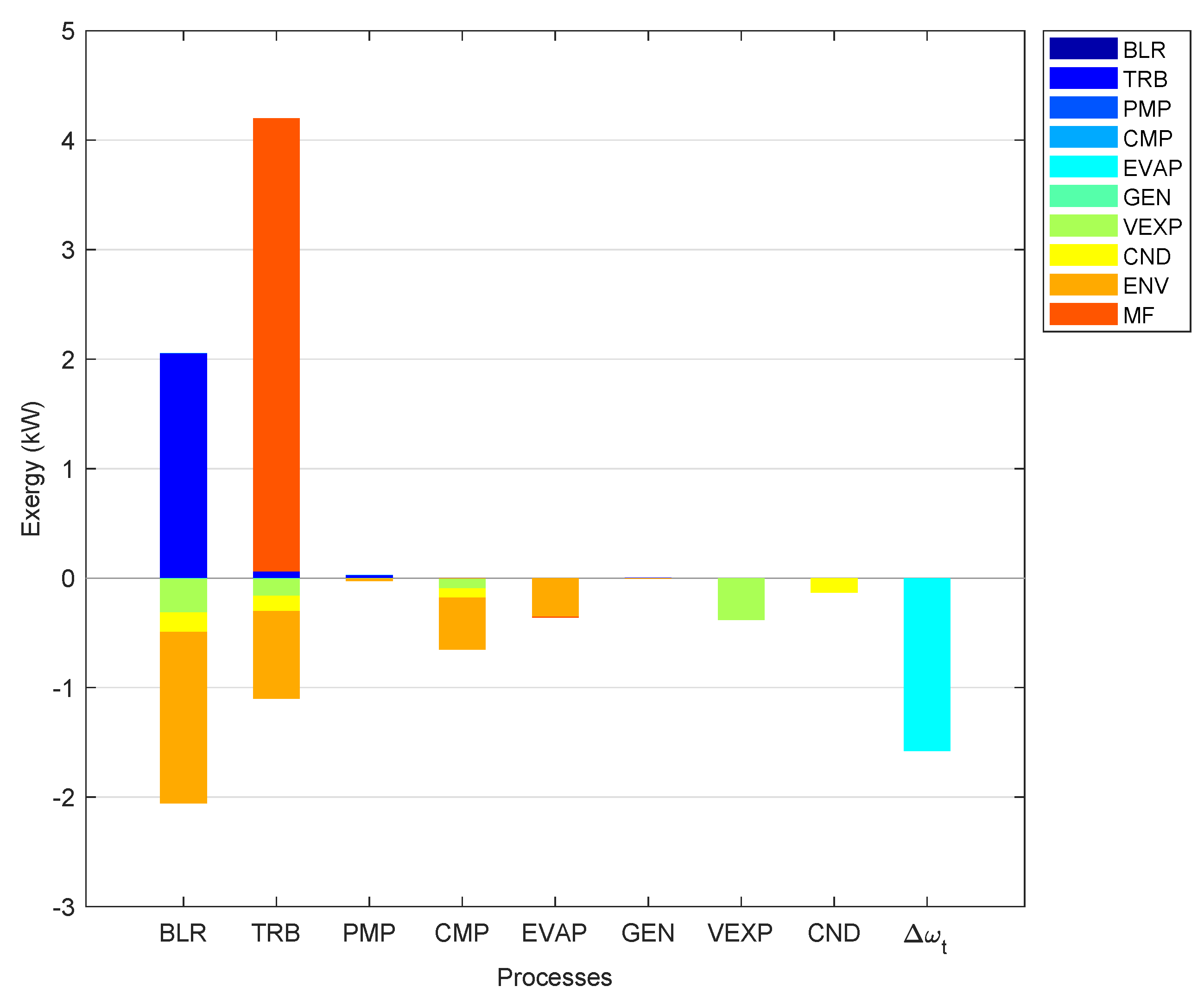
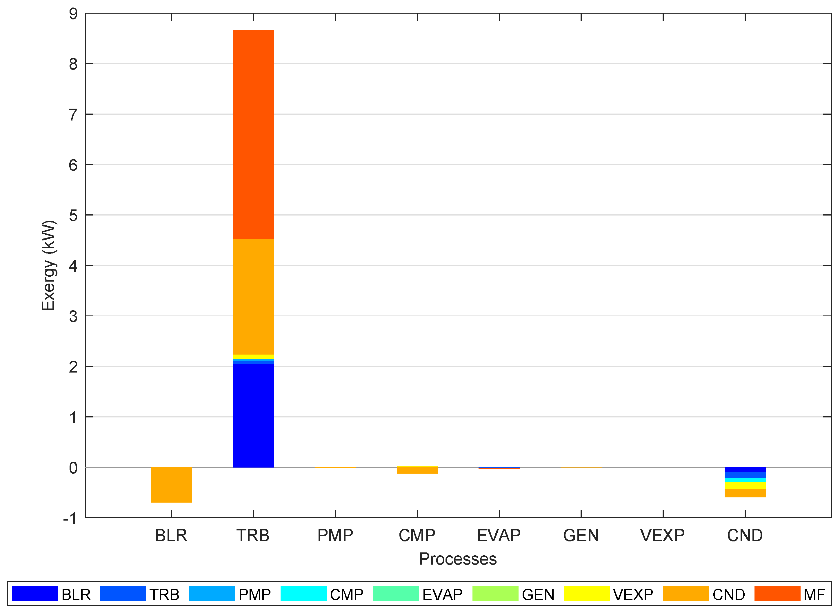
As shown in Figure 2, the increase in process irreversibilities due to variation in end products can be significant. This is because the thermoeconomic diagnosis has usually been applied to plants with constant production. This formulation does not contemplate systems with several final products that could vary or with systems whose external resources can be pre-fixed.

The new approach analyzes the causes of increased waste generation, Equation (17), and its cost in terms of additional resource consumption, Equation (19). Moreover, special care is taken to separate the costs of internal process malfunctions $M{F}^{*}$ from those caused by additional waste generation $M{R}^{*}$, and the cost of final product generation is evaluated taking into account both internal and external irreversibilities, Equation (20).

Table 5 summarizes the results and compares fuel impact and effective fuel impact for the different simulations. In the first two cases, resource consumption is constant, but a malfunction in the turbine and compressor causes a reduction in production and an increase in total irreversibility. The effective fuel impact indicates the amount of resources that would have been consumed if production had been maintained, which, in the case of the turbine, is 7%. In the following two cases, there is a reduction in resource consumption, which, in this example, is a lack of waste heat utilization. In the case of the condenser temperature increase, the cooling output is reduced. The effective fuel impact measures the cost of the malfunction, which is equal to the fuel needed to maintain production, which would be 20% higher. In the case of pressure reduction (temperature decrease) in the boiler, the effect is similar. However, in this case, the effective fuel impact is less than 1%. These examples show that the new ${\mathcal{M}}_T$ indicator is a more realistic measure of malfunction costs than the original fuel impact index.

Table 5. Diagnosis summary results of the ORC-VCR system (kW).

State	$\mathbf{\Delta }{\mathit{F}}_{\mathit{T}}$	${\mathcal{M}}_{\mathit{T}}$	$\mathbf{\Delta }\mathit{I}$	$\mathbf{\Delta }{\mathit{\omega }}_{\mathit{t}}$	$\mathbf{\Delta }{\mathit{\omega }}_{\mathit{t}}^{*}$
ETAT75	0.000	7.231	3.820	−3.820	−7.231
ETAC78	0.000	2.387	1.000	−1.000	−2.387
TCND35	−3.300	23.793	2.270	−5.570	−27.093
TBLR85	−6.070	0.655	−4.510	−1.560	−6.725

In summary, for thermoeconomic diagnosis, the first step should be identifying internal system failures ($MF$), not irreversibilities, as these include malfunctions caused by other equipment and those induced by production changes. Once the failure has been identified, we must quantify its cost in terms of additional fuel consumption, namely:

• The part due to internal irreversibilities that have produced $M{F}^{*}$.
• The part associated with waste generation $M{R}^{*}$.
• The part associated with the variation of the final product $\Delta {\omega }_t^{*}$.

The methodology is illustrated with an example in which different simulations are analyzed, and their feasibility is demonstrated.

In conclusion, Circular thermoeconomic diagnosis is a thermodynamic monitoring methodology that analyzes any deviations from actual operating conditions, identifies possible malfunctions and assesses the effect of each failure on the additional consumption of system resources. It can be applied to a wide range of energy systems to define new plant operation and control strategies, including analyzing additional waste generation. As the introduction mentions, thermoeconomic diagnosis mainly covers the primary waste. Therefore, a possible research field is to analyze the secondary and tertiary waste extending the system’s boundaries.

Among the perspectives of this work is the application of thermoeconomic diagnosis to a new renewable energy production plant to help define rules and criteria for operation and to develop an IA monitoring system that warns of any problem that causes a decrease in its performance compared to the plant’s reference state.

References

- Webster, K. The Circular Economy: A Wealth of Flows; Ellen MacArthur Foundation: Cowes, UK, 2015. [Google Scholar]
- McDonough, W.; Braungart, M. Cradle to Cradle: Remaking the Way We Make Things; Macmillan: New York, NY, USA, 2003. [Google Scholar]
- Benyus, J.M. Biomimicry: Innovation Inspired by Nature; William Morrow and Company: New York, NY, USA, 1997. [Google Scholar]
- Wijkman, A.; Skånberg, K. The Circular Economy and Benefits for Society: Jobs and Climate, Clear Winners in an Economy Based on Renewable Energy and Resource Efficiency; A Club of Rome Report; Club of Rome: Zurich, Switzerland, 2017. [Google Scholar]
- ISO 50045; Technical Guidelines for the Evaluation of Energy Savings of Thermal Power Plants. ISO: Geneva, Switzerland, 2019.
- Lozano, M.; Bartolome, J.; Valero, A.; Reini, M. Thermoeconomic Diagnosis of Energy Systems. In Proceedings of the Flowers 94: Florence World Energy Research Symposium, Florence, Italy, 6–8 July 1994. [Google Scholar]
- Lazzaretto, A.; Toffolo, A. A critical review of the thermoeconomic diagnosis methodologies for the location of causes of malfunctions in energy Systems. J. Energy Resour. Technol. Trans. ASME 2006, 128, 335–341. [Google Scholar] [CrossRef]
- Reini, M.; Lazareto, A.; Macor, A. Average Structural and Marginal Cost as result of a unified formulation of the thermoeconomic problem. In Proceedings of the Second Law Analysis of Energy Systems—Towards the 21st Century, Rome, Italy, 5–7 July 1995. [Google Scholar]
- Kotas, T. The Exergy Method of Thermal Plant Analysis; Butterworths: London, UK, 1996. [Google Scholar]
- Valero, A.; Correas, L.; Zaleta, A.; Lazzaretto, A.; Verda, V.; Reini, M.; Rangel, V. On the thermoeconomic approach to the diagnosis of energy system malfunctions. Part 2. Malfunction definitions and assessment. Energy 2004, 29, 1889–1907. [Google Scholar] [CrossRef]
- Valero, A.; Correas, L.; Lazzaretto, A.; Rangel, V.; Reini, M.; Taccani, R.; Toffolo, A.; Verda, V.; Zaleta, A. Thermoeconomic Philosophy Applied to Operating Analysis and Diagnosis of Energy Utility Systems. Int. J. Thermodyn. 2004, 7, 33–39. [Google Scholar]
- Toffolo, A.; Lazzaretto, A. On the Thermoeconomic Approach to the Diagnosis of Energy System Malfunctions—Indicators to Diagnose Malfunctions: Application of a New Indicator for the Location of Causes. Int. J. Thermodyn. 2004, 7, 41–49. [Google Scholar]
- Reini, M.; Taccani, R. On the Thermoeconomic Approach to the Diagnosis of Energy System Malfunctions. The Role of the Fuel Impact Formula. Int. J. Thermodyn. 2004, 7, 61–72. [Google Scholar]
- Verda, V. Thermoeconomic Analysis and Diagnosis of Energy Utility Systems—From Diagnosis to Prognosis. Int. J. Thermodyn. 2004, 7, 73–83. [Google Scholar]
- Correas, L. On the Thermoeconomic Approach to the Diagnosis of Energy System Malfunctions—Suitability to Real-Time Monitoring. Int. J. Thermodyn. 2004, 7, 85–94. [Google Scholar]
- Sciubba, E. Hybrid Semi-Quantitative Monitoring and Diagnostics of Energy Conversion Processes. Int. J. Thermodyn. 2004, 7, 95–106. [Google Scholar]
- Zhang, C.; Chen, S.; Zheng, C.; Lou, X. Thermoeconomic diagnosis of a coal fired power plant. Energy Convers. Manag. 2007, 48, 405–419. [Google Scholar] [CrossRef]
- Zaleta-Aguilar, A.; Olivares-Arriaga, A.; Cano-Andrade, S.; Rodriguez-Alejandro, D.A. β-characterization by irreversibility analysis: A thermoeconomic diagnosis method. Energy 2016, 111, 850–858. [Google Scholar] [CrossRef]
- Piacentino, A.; Talamo, M. Innovative thermoeconomic diagnosis of multiple faults in air conditioning units: Methodological improvements and increased reliability of results. Int. J. Refrig. 2013, 36, 2343–2365. [Google Scholar] [CrossRef]
- Ommen, T.; Sigthorsson, O.; Elmegaard, B. Two Thermoeconomic Diagnosis Methods Applied to Representative Operating Data of a Commercial Transcritical Refrigeration Plant. Entropy 2017, 19, 69. [Google Scholar] [CrossRef]
- Picallo-Perez, A.; Sala-Lizarraga, J.M.; Portillo-Valdes, L. Development of a tool based on thermoeconomics for control and diagnosis building thermal facilities. Energy 2022, 239, 122304. [Google Scholar] [CrossRef]
- Rúa-Orozco, D.J.; Venturini, O.J.; Escobar Palacio, J.C.; Almazán del Olmo, O. A new methodology of thermodynamic diagnosis, using the thermoeconomic method together with an artificial neural network (ANN): A case study of an externally fired gas turbine (EFGT). Energy 2017, 123, 20–35. [Google Scholar] [CrossRef]
- Keshavarzian, S.; Rocco, M.V.; Colombo, E. Thermoeconomic diagnosis and malfunction decomposition: Methodology improvement of the Thermoeconomic Input-Output Analysis (TIOA). Energy Convers. Manag. 2018, 157, 644–655. [Google Scholar] [CrossRef]
- Mendes, T.; Venturini, O.J.; da Silva, J.A.M.; Orozco, D.J.R.; Pirani, M.J. Disaggregation models for the thermoeconomic diagnosis of a vapor compression refrigeration system. Energy 2020, 193, 116731. [Google Scholar] [CrossRef]
- Castro-Hernández, S.; López-Arenas, T.; Torres-González, E.; Lugo-Méndez, H.; Lugo-Leyte, R. Thermoeconomic Diagnosis of the Sequential Combustion Gas Turbine ABB/Alstom GT24. Energies 2022, 15, 631. [Google Scholar] [CrossRef]
- Valero, A.; Torres, C. Circular Thermoeconomics: A Waste Cost Accounting Theory. In Advances in Thermodynamics and Circular Thermoeconomy; Feidt, M., Valero, A., Eds.; Willey: London, UK, 2023. [Google Scholar]
- Torres, C.; Valero, A. The Exergy Cost Theory Revisited. Energies 2021, 14, 1594. [Google Scholar] [CrossRef]
- Szargut, J. Exergy Method: Technical and Ecological Applications; WIT Press: Southampton, UK, 2005. [Google Scholar]
- Tsatsaronis, G.; Winhold, M. Exergoeconomic analysis and evaluation of energy-conversion plants. Part I—A new general methodology. Energy 1985, 10, 69–80. [Google Scholar] [CrossRef]
- Bisson, K.; Proops, J. Waste in Ecological Economics; Edward Elgar Publishing: Northampton, MA, USA, 2002. [Google Scholar]
- Sciuba, E. A Thermodynamically Correct Treatment of Externalities with an Exergy-Based Numeraire. Sustainability 2012, 4, 933–957. [Google Scholar] [CrossRef]
- Nakamura, S.; Kondo, Y. Waste Input-Output Analysis: Concepts and Application to Industrial Ecology; Springer: Tokyo, Japan, 2009. [Google Scholar]
- Liao, W.; Heijungs, R.; Huppes, G. Thermodynamic analysis of human–environment systems: A review focused on industrial ecology. Ecol. Model. 2012, 228, 76–88. [Google Scholar] [CrossRef]
- Graedel, T.E.; Allenby, B.R. Industrial Ecology; Prentice Hall: Englewood Cliffs, NJ, USA, 1995. [Google Scholar]
- Dos Santos, M.T.; Park, S.W. Sustainability and biophysics basis of technical and economic processes: A survey of the reconciliation by thermodynamics. Renew. Sustain. Energy Rev. 2012, 23, 261–271. [Google Scholar] [CrossRef]
- Cecchin, A.; Salomone, R.; Deutz, P.; Raggi, A.; Cutaia, L. Relating Industrial Symbiosis and Circular Economy to the Sustainable Development Debate. In Industrial Symbiosis for the Circular Economy: Operational Experiences, Best Practices and Obstacles to a Collaborative Business Approach; Salomone, R., Cecchin, A., Deutz, P., Raggi, A., Cutaia, L., Eds.; Springer International Publishing: Cham, Switzerland, 2020; pp. 1–25. [Google Scholar] [CrossRef]
- Torres, C.; Valero, A.; Rangel, V.; Zaleta, A. On the cost formation process of the residues. Energy 2008, 33, 144–152. [Google Scholar] [CrossRef]
- TaesLab Toolbox. CIRCE Institute. University of Zaragoza. Available online: https://exergoecology.com/TaesLab (accessed on 20 August 2023).
- Pektezel, O.; Acar, H.I. Energy and Exergy Analysis of Combined Organic Rankine Cycle-Single and Dual Evaporator Vapor Compression Refrigeration Cycle. Appl. Sci. 2019, 23, 5028. [Google Scholar] [CrossRef]
- F-Chart Software, Engineering Equation Solver (EES). Available online: https://fchartsoftware.com/ees (accessed on 20 August 2023).
Disclaimer/Publisher’s Note: The statements, opinions and data contained in all publications are solely those of the individual author(s) and contributor(s) and not of MDPI and/or the editor(s). MDPI and/or the editor(s) disclaim responsibility for any injury to people or property resulting from any ideas, methods, instructions or products referred to in the content. |
© 2023 by the authors. Licensee MDPI, Basel, Switzerland. This article is an open access article distributed under the terms and conditions of the Creative Commons Attribution (CC BY) license (https://creativecommons.org/licenses/by/4.0/).