A Wind Power Forecasting Model Using LSTM Optimized by the Modified Bald Eagle Search Algorithm

Abstract

High-precision forecasting of short-term wind power (WP) is integral for wind farms, the safe dispatch of power systems, and the stable operation of the power grid. Currently, the data related to the operation and maintenance of wind farms mainly comes from the Supervisory Control and Data Acquisition (SCADA) systems, with certain information about the operating characteristics of wind turbines being readable in the SCADA data. In short-term WP forecasting, Long Short-Term Memory (LSTM) is a commonly used in-depth learning method. In the present study, an optimized LSTM based on the modified bald eagle search (MBES) algorithm was established to construct an MBES-LSTM model, a short-term WP forecasting model to make predictions, so as to address the problem that the selection of LSTM hyperparameters may affect the forecasting results. After preprocessing the WP data acquired by SCADA, the MBES-LSTM model was used to forecast the WP. The experimental results reveal that, compared with the PSO-RBF, PSO-SVM, LSTM, PSO-LSTM, and BES-LSTM forecasting models, the MBES-LSTM model could effectively improve the accuracy of WP forecasting for wind farms.

1. Introduction

The development of renewable energy can effectively reduce the deficiency of global energy and reduce environmental pollution [1]. Notably, wind energy has become one of the fastest-growing renewable energy sources [2], serving as an environmentally friendly and clean energy source that can meet the requirements of human sustainable development [3]. According to statistics related to WT (wind turbine) released by the World Wind Energy Association (WWEA) in early 2021, the total installed capacity of global WT in 2020 reached 744 GW [4].

Despite the extensive promotion of WP, bringing about significant economic benefits, wind farms are also facing several challenges. Since the wind farms’ output power can be volatile and uncertain, after the wind farm is connected to the grid, there will be certain disturbances to the safe operation of the power system [5]. To overcome such problems, accurate forecasting of the wind farm output power is necessary. Through forecasting, WP fluctuations can be determined in advance. As such, corresponding countermeasures can also be prepared in advance, and a reasonable power generation plan can be arranged, which not only ensures the safety of the grid, but also improves its reliability [6].

In recent years, researchers have conducted extensive research on WP forecasting using numerous mainstream models, including physical models [7], statistical models [8,9], and artificial intelligence (AI) models [10,11], among which AI models are the most widely studied.

AI models usually establish a high-dimensional nonlinear function to fit WP by minimizing training errors [12]. The more widely used methods are mainly machine learning (ML) methods and artificial neural network (ANN) methods. ML methods mainly include Support Vector Regression (SVR), Least Square Support Vector Machine (LSSVM), and Extreme Learning Machine (ELM) networks [13]. Kuilin Chen et al. [14] used an unscented Kalman filter (UKF) for integration with SVR to establish an SVR-UKF forecasting model, which improved the forecasting accuracy of the SVR model. The ANN acts as a parallel processor with the ability of efficiently storing and figuring out experimental knowledge; it is suitable for solving complex nonlinear problems [15]. D. Huang et al. [16] used GA and BP neural networks to forecast the WP of a wind farm. This GA-BP model was beneficial in improving the correctness of WP forecasting. P. Guo et al. [17] used GA to optimize the hyper-parameters of RBF and to predict the WP of a wind farm. As the theories and technology of neural networks have gradually developed and matured, more researchers have applied deep neural networks (DNN), such as convolutional neural networks (CNN) [18], deep belief networks (DBN) [19], and RNN [20] to predict the WP of wind farms.

LSTM as a form of RNN, has been demonstrated to be suitable for analyzing long series data, and there have been an increasing number of studies on the forecasting of WP based on LSTM networks. In order to construct an LSTM network model that meets the requirements, it is necessary to adjust the relevant hyperparameters, and researchers often set the parameters according to their actual experience and priori knowledge. For different problems, it may be necessary to repeatedly manually tune the relevant parameters.

To address such issues, the parameters of LSTM are optimized using the MEBS algorithm; thus, constructing the MBES-LSTM forecasting model. The experimental results reveal that the optimized forecasting model can better predict the trend of WP and provide technical support for the refinement of wind farm management. The main contributions are highlighted as follows:

(1)

The original BES algorithm was improved, and the improved BES algorithm was tested.

(2)

The wind farm data collected by the SCADA system was cleaned and filtered to form a sample set and processed by means of an empirical mode decomposition (EMD) method.

(3)

The parameters of the LSTM such as iteration number $T_{iter}$, learning rate $L_R$, number of the first layer $L_1$, number of the second layer $L_2$, were optimized by the MBES algorithm, and the MBES-LSTM forecasting model was subsequently constructed.

(4)

The processed WP data was used as the test sample with the PSO-RBF, PSO-SVM, LSTM, PSO-LSTM, BES-LSTM, and MBES-LSTM models to predict and compare performance.

The balance of this paper is organized as follows: Section 2 describes the LSTM, BES, and MBES algorithm. Evaluation index, MBES-LSTM forecasting model, SCADA data preprocess, and relevant parameter settings are introduced in Section 3. Section 4 provides some graphical results, along with analysis. Finally, Section 5 concludes this paper.

2. Description of LSTM, BES, and MBES

2.1. LSTM

LSTM is a special type of RNN, of which the hidden layer is composed of one or more memory cells, and each memory cell includes a forget gate, an input gate, and an output gate [21]; its structure is shown in Figure 1.

Figure 1. Structure of LSTM.

(1) Forget gate: The forget gate $f_t$ is responsible for controlling whether the long-term state $c$ continues to be preserved, and is jointly determined by the input $x_t$ of the current moment $t$ and the output $h_{t-1}$ of the previous moment $t-1$. The relevant formula is as follows:

$$f_t=\sigma \left(W_f\times \left[h_{t-1}, x_t\right]+B_f\right)$$

(1)

where $W_f$ represents the weight matrix of the forget gate; $B_f$ represents the bias term; and $\sigma (•)$ represents the sigmoid function.

(2) Input gate: The function of the input gate is to establish a new unit state $\tilde{c}$, perform related processing therein, and control how much information is added. The calculation formula is as follows:

$$i_t=\sigma \left(W_i\times \left[h_{t-1}, x_t\right]+B_i\right)$$

(2)

$${\tilde{c}}_t=tanh\left(W_c\times \left[h_{t-1}, x_t\right]+B_c\right)$$

(3)

where $i_t$ is the input gate result; $W_i$ represents the weight matrix of the input gate; $B_i$ represents the bias of the input gate; $\tilde{c}$ represents the current input cell state; $W_c$ represents the weight matrix; and $B_c$ represents the bias of the cell state. The matrix $[h_{t-1}, x_t]$ is composed of two vectors, the output $h_{t-1}$ at the previous moment $t-1$ and the input $x_t$ at the current moment $t$. $\sigma (•)$ is the sigmoid activation function and $\mathit{tanh}(•)$ is a double tangent function.

(3) Output gate: In the output gate, the output $h_{t-1}$ of the previous moment $t-1$ and the input $x_t$ of the current moment $t$ are used to output $f_t$ through a sigmoid function $\sigma (•)$, namely:

$$O_t=\sigma \left(W_o\times \left[h_{t-1}, x_t\right]+B_o\right)$$

(4)

$$c_t=f_t\times c_{t-1}+i_t\circ {\tilde{c}}_t$$

(5)

$$h_t=o_t\times tanh(c_t)$$

(6)

where $W_o$ represents the weight matrix of the output gate; and $B_o$ represents the bias term of the output gate.

In the LSTM structure, due to the unique three-gate structure and the existence of the hidden state with storage function, LSTM can better reveal long-term historical data, thereby solving the issue of long-term dependence. First, the hidden state $C_t$ of the current moment $t$ uses the forget gate to control which information in the hidden state $C_{t-1}$ of the last moment $t-1$ needs to be discarded, and which information can continue to be retained. Second, the structure discards certain information in the hidden state $C_t$ and the forget gate, and learns new information through the input gate. Third, after a series of calculations, the cell state $C_t$ is updated. Here, LSTM uses the output gate, cell state $C_t$, and a tanh layer to determine the final output value $h_t$.

2.2. BES Algorithm

The BES is a new meta-heuristic optimization algorithm established in 2020 by H. A. Alsattar, who was inspired by the hunting behavior of bald eagles [22]. Bald eagles are found throughout North America and have sharp eyesight and significantly high observation ability during flight [23]. Taking salmon predation as an example, the bald eagle will first select a search space based on the distribution density of individuals and populations to salmon and fly towards a specific area; next, the bald eagle will search the water surface in the selected search space until a suitable prey is found; finally, the bald eagle will gradually change the flying altitude, dive down quickly, and successfully catch salmon and other prey from the water. The BES algorithm simulates the prey-preying behavior of this condor and divides it into three stages: select stage, search stage, and swooping stage, as shown in Figure 2.

Figure 2. Diagram of the BES for the three main phases of hunting (S1—selecting phase; S2—searching phase; S3—swooping phase). (a) Selecting phase; (b) Search and swooping phase.

(1) Selecting phase: In the selecting phase, the search area is randomly selected by the bald eagle looking for the area with the most prey. The updated description of the bald eagle’s position at this phase is:

$${\mathit{L}}_{new}^i={\mathit{L}}_{best}^{}+\alpha \cdot r\left({\mathit{L}}_{mean}^{}-{\mathit{L}}_{}^i\right)$$

(7)

where, ${\mathit{L}}_{new}^i$ represents the latest location of the i-th bald eagle, and ${\mathit{L}}_{best}^{}$ is the current optimal position; ${\mathit{L}}^i$ represents the location of the i-th bald eagle; ${\mathit{L}}_{mean}^{}$ is the evenly distributed bald eagle’s position after the previous search; $\alpha \in \left[1.5, 2\right]$ is the parameter which controls the positions change; and $r\in \left(0, 1\right)$ is an arbitrary number

(2) Searching phase: In the searching phase, the bald eagle flies in a conical spiral in the selected search space, looking for prey. In the conical spiral space, the bald eagle moves in a different course to accelerate its searching speed and find the best dive capture location. The updated description of the spiral flight position of the bald eagle is:

$$\theta (i)=\beta \times \pi \times random\left(0,1\right)$$

(8)

$$r(i)=\theta (i)+\gamma \times random\left(0,1\right)$$

(9)

$$x\times r(i)=r(i)\times sin[\theta (i)]$$

(10)

$$y\times r(i)=r(i)\times cos[\theta (i)]$$

(11)

$$x(i)=\frac{x\times r(i)}{max(\left|x\times r\right|)}$$

(12)

$$y(i)=\frac{y\times r(i)}{max(\left|y\times r\right|)}$$

(13)

where $\theta (i)$ is the polar angle of the spiral equation; $r(i)$ is the polar diameter of the spiral equation; $\beta \in \left(0, 5\right)$ and $\gamma \in \left(0.5, 2\right)$ are the parameters that control the spiral trajectory; $x(i)$ and $y(i)$ represent the bald eagle’s location in polar coordinates, with both values being (−1, 1). The bald eagle’s position is updated as follows:

$${\mathit{L}}_{new}^i={\mathit{L}}_{}^i+x(i)\times \left({\mathit{L}}_{}^i-{\mathit{L}}_{mean}^{}\right)+y(i)\times \left({\mathit{L}}_{}^i-{\mathit{L}}_{}^{i+1}\right)$$

(14)

where ${\mathit{L}}_{}^{i+1}$ is the next updated location of the i-th bald eagle.

(3) Swooping phase: After the bald eagle locks onto a target, it quickly dives from the best position and flies towards the target. The movement state of this phase is still used, and the polar coordinate equation can be denoted as follows:

$${\mathit{L}}_{new}^i=rand(0,1)\times {\mathit{L}}_{best}^{}+{\delta }_x+{\delta }_y$$

(15)

$${\delta }_x=x1(i)\times ({\mathit{L}}^i-{\lambda }_1\times {\mathit{L}}_{mean}), {\lambda }_1\in [1,2]$$

(16)

$${\delta }_y=y1(i)\times ({\mathit{L}}^i-{\lambda }_2\times {\mathit{L}}_{best}), {\lambda }_2\in [1,2]$$

(17)

where, ${\lambda }_1$ and ${\lambda }_2$ represents best position and center position, respectively.

2.3. MBES Algorithm

The MBES algorithm is an improved version of the original BES algorithm. In the selection phase, the parameter $\alpha$ in Formula (7) was optimized to no longer be a fixed value between [1.5, 2], which can be expressed by the following formula:

$$a_t=exp\left(\frac{T-t}{T}\right)-1$$

(18)

$${\mathit{L}}_{new}^i={\mathit{L}}_{best}+a_t\times r\left({\mathit{L}}_{mean}-L_{}^i\right)$$

(19)

where $a_t$ is the bald eagle’s position change control parameter; $t$ represents the current iteration number; $T$ is the maximum iteration number.

The MBES algorithm was tested and evaluated using different benchmark functions; the parameters of all compared algorithms, such as particle swarm optimization (PSO), grey wolf optimizer (GWO), whale optimization algorithm (WOA), BES, and MBES are shown in Table 1. Table 2 presents the name and parameter settings of the benchmark functions.

Table 1. Parameter value of PSO, GWO, WOA, BES, and MBES.

Algorithm	Parameter Setting
Common setting	Maximum iteration N = 200
	population size: P = 10
	Runs: r = 20
	Probability Pr = 0.5
PSO	V1 = 2
	V2 = 2
	W = 0.9
GWO	m1 = 0.3
WOA	P1 = 3
	P2 = 5
BES	α = 2
	λ1 = 2, λ2 = 2
	a = 10
	R = 1.5
MBES	λ1 = 2, λ2 = 2
	a = 10
	R = 1.5

Table 2. Parameter settings of test functions.

Test Function	Function Name	D	Range	fopt
(1) Unimodal test functions
$F_1\left(x\right)={\displaystyle {\sum }_{i=1}^D{\left(x_i+0.5\right)}^2}$	Step	30	[−100, 100]	0
$F_2\left(x\right)={\displaystyle {\sum }_{i=1}^{D}i{x}_i^4+random\left[0,1\right)}$	Quartic	30	[−1.28, 1.28]	0
(2) Multimodal test functions
$F_3\left(x\right)=20+e-20\exp \left(-20\sqrt{\left(1/D\right){\sum }_{\mathrm{i}=1}^D{x}_i^2})-\exp ((1/D){\displaystyle {\sum }_{i=1}^D\cos \left(2\pi x_i\right)}\right)$	Ackley	30	[−32, 32]	0
$F_4\left(x\right)=\left(1/4000\right){\displaystyle {\sum }_{i=1}^D{\left(x_i^{}-100\right)}^2}-\left({\displaystyle {\prod }_{i=1}^D\cos \left(\frac{x_i-100}{\sqrt{i}}\right)}\right)+1$	Griewank	30	[−600, 600]	0
$\begin{array}{l}{F}_5\left(x\right)=\left(\pi /D\right)\\ \left\{10{\sin }^2\left(\pi y_i\right)+{\displaystyle {\sum }_{i=1}^D{\left(y_i-1\right)}^2\left[1+10{\sin }^2\left(\pi y_{i+1}\right)\right]+\left(y_D-1\right)}\right\}\\ +{\displaystyle {\sum }_{i=1}^{D}u\left(x_i,10,100,4\right)}\end{array}$	Penalized	30	[−50, 50]	0
(3) Composite benchmark functions
$F_6\left(x\right)={\left(\left(1/500\right)+{\displaystyle {\sum }_{j=1}^{25}\left(1/\left(j+{\displaystyle {\sum }_{i=1}^2{\left(x_i-a_{ij}\right)}^6}\right)\right)}\right)}^{-1}$	Foxholes	2	[−65.53, 65.53]	0.998004
$F_7\left(x\right)=-{\displaystyle {\sum }_{i=1}^4\left(c_i\exp {\left(-{\displaystyle {\sum }_{j-1}^6{a}_{ij}\left(x_i-p_{ij}\right)}\right)}^2\right)}$	Martman 6	6	[0, 1]	−3.322
$F_8\left(x\right)=-{\displaystyle {\sum }_{i=1}^{10}{\left[\left(X-a_i\right){\left(X-a_i\right)}^T+c_i\right]}^{-1}}$	Langerman 10	4	[0, 10]	−10.5364

The relevant statistical experiment results of selecting each algorithm to run 20 times independently in the benchmark function are shown in Table 3 (unimodal benchmark functions), Table 4 (multimodal benchmark functions), and Table 5 (composite benchmark functions).

Table 3. Results for unimodal benchmark functions.

Function	Statistics	PSO	GWO	WOA	BES	MBES
F1	Best	3.462 × 10−1	1.122 × 10−1	3.667 × 10−4	2.341 × 10−16	0
	Worst	5.183 × 103	6.135 × 104	6.006 × 104	7.288	7.279
	Average	6.021 × 101	2.294 × 102	2.117 × 102	1.981 × 10−1	8.983 × 10−2
	Std.	3.101 × 102	2.828 × 103	2.854 × 103	7.723 × 10−1	6.035 × 10−1
F2	Best	4.169 × 10−3	2.570 × 10−4	6.913 × 10−4	3.923 × 10−5	1.557 × 10−5
	Worst	6.976 × 101	1.011 × 102	9.312 × 101	5.994 × 10−2	2.665 × 10−2
	Average	9.507 × 10−1	2.593 × 10−1	2.735 × 10−1	2.968 × 10−4	1.301 × 10−4
	Std.	7.123	3.973	4.054	2.175 × 10−3	1.011 × 10−3

Table 4. Results for multimodal benchmark functions.

Function	Statistics	PSO	GWO	WOA	BES	MBES
F3	Best	1.644 × 10−1	1.066 × 10−14	3.730 × 10−15	8.882 × 10−16	8.882 × 10−16
	Worst	1.876 × 101	2.047 × 101	2.057 × 101	7.817 × 10−4	2.325 × 10−8
	Average	1.812	2.841 × 10−1	2.297 × 10−1	7.817 × 10−7	2.325 × 10−11
	Std.	2.241	1.889	1.731	2.472 × 10−5	7.353 × 10−10
F4	Best	4.4484 × 10−2	0	0	0	0
	Worst	3.3475	6.3476 × 102	5.4016 × 102	1.3714	1.0657
	Average	3.7099 × 10−1	2.4048	2.0291	1.7522 × 10−3	1.0663 × 10−3
	Std.	3.9847 × 10−1	2.9049 × 101	2.8352 × 101	4.4912 × 10−2	3.3700 × 10−2
F5	Best	9.934 × 10−2	1.583 × 10−2	4.714 × 10−5	4.285 × 10−19	1.572 × 10−32
	Worst	8.002 × 106	4.691 × 108	4.621 × 108	1.510	1.462
	Average	1.095 × 104	1.074 × 106	1.188 × 106	1.265 × 10−2	8.612 × 10−3
	Std.	2.603 × 105	1.875 × 107	1.994 × 107	9.636 × 10−2	8.345 × 10−2

Table 5. Results for composite benchmark functions.

Function	Statistics	PSO	GWO	WOA	BES	MBES
F6	Best	9.980 × 101	2.570	1.048	5.633	4.702 × 10−1
	Worst	1.510	5.387 × 101	3.579 × 101	1.351 × 101	1.150 × 101
	Average	9.989 × 10−1	2.669	1.199	5.690	4.738
	Std.	1.873 × 10−2	1.676	1.263	3.787 × 10−1	3.174 × 10−1
F7	Best	3.979 × 10−1	3.979 × 10−1	3.979 × 10−1	3.979 × 10−1	3.979 × 10−1
	Worst	4.269 × 10−1	8.117 × 10−1	8.530 × 10−1	7.572 × 10−1	6.451 × 10−1
	Average	3.980 × 10−1	3.997 × 10−1	3.997 × 10−1	3.988 × 10−1	3.983 × 10−1
	Std.	1.626 × 10−3	1.967 × 10−2	1.910 × 10−2	1.355 × 10−2	8.160 × 10−3
F8	Best	−1.0536 × 101	−1.0536 × 101	−1.0536 × 101	−1.0536 × 101	−1.0536 × 101
	Worst	−1.5670	−1.0484	−1.7075	−2.7215	−1.8866
	Average	−1.0344 × 101	−8.7332	−1.0424 × 101	−1.0488 × 101	−1.0495 × 101
	Std.	1.0742	1.9366	8.0145 × 10−1	3.8490 × 10−1	5.2253 × 10−1

Figure 3 presents the qualitative metrics for the F1–F8 functions, including 2D views of the functions and convergence curves. For the convergence curves in Figure 3, the red line represents the MBES and the blue line represents the BES. As can be seen, the MBES’s speed of convergence is faster than the others.

Figure 3. Qualitative metrics for the benchmark functions: 2D views and convergence curves of the functions. (a) F1; (b) F2; (c) F3; (d) F4; (e) F5; (f) F6; (g) F7; (h) F8.

3. WP Forecast

3.1. MBES-LSTM Forecasting Model

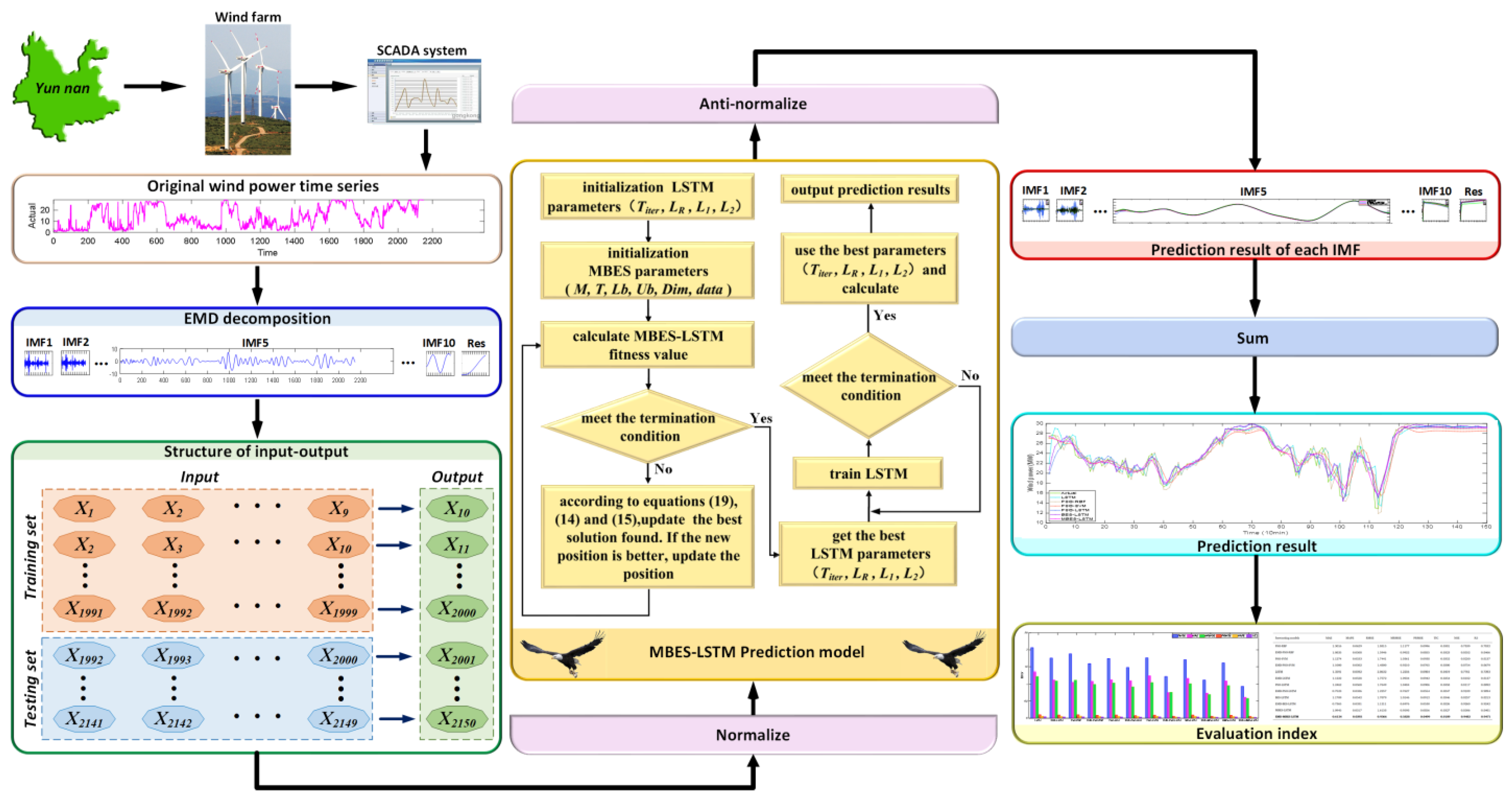
To reduce forecasting errors, SCADA data is decomposed using the EMD method after preprocessing. The flow chart of the MBES-LSTM WP forecasting model based on the EMD is shown in Figure 4, and the specific steps were as follows:

Figure 4. Forecasting process of the proposed model.

Step 1: The EMD method was used to decompose the pre-processed WP time series data and to decompose the data into the intrinsic mode function (IMF).

Step 2: The data of each IMF was divided into a training set and a test set.

Step 3: The decomposition data from each IMF was normalized.

Step 4: The MBES-LSTM model was used for training and forecasting, respectively, and in this step:

(1)

The LSTM $\{T_{iter},L_R,L_1^{},L_2^{}\}$ parameter and the MBES algorithm parameters, including the bald eagle population $N$, the maximum iterations $M$, the upper limit of argument $Ub$, the lower limit of argument $Lb$, the dimension $D$, and the sample data were initialized.

(2)

The data of the fitness value was calculated. The mean square error obtained by training the LSTM network was used as the fitness value, and the value was updated in real-time as the bald eagle continued to operate; within the iteration range, Formulas (14), (15), and (19) were used to calculate the position of the bald eagle. If the current new position was better, the old position was updated.

(3)

According to the optimal parameter combination, the LSTM network was trained, and testing samples were used to forecast and save the result of each IMF.

Step 5: The results of each IMF from Step 4 were anti-normalized.

Step 6: By linearly superimposing the forecasting results of each IMF, the final forecasting result was obtained.

Step 7: The relevant evaluation metrics were calculated.

3.2. Data Preprocessing and EMD Decomposition

In the present study, the actual operational SCADA data of a wind farm in Yunnan, China, from 1 August 2018 to 31 August 2018, was selected for the analysis of the calculation examples. The time resolution of the data was ten minutes. After data cleaning, the first 2150 groups were taken as experimental samples. The relevant features of the samples are shown in Table 6.

Table 6. Attributes of training set and test set samples.

	Training Set	Testing Set
number of samples	2000 (pcs)	150 (pcs)
minimum value	0.5660 (MW)	13.2090 (MW)
maximum value	29.3640 (MW)	29.3460 (MW)
average value	13.2264 (MW)	24.4299 (MW)

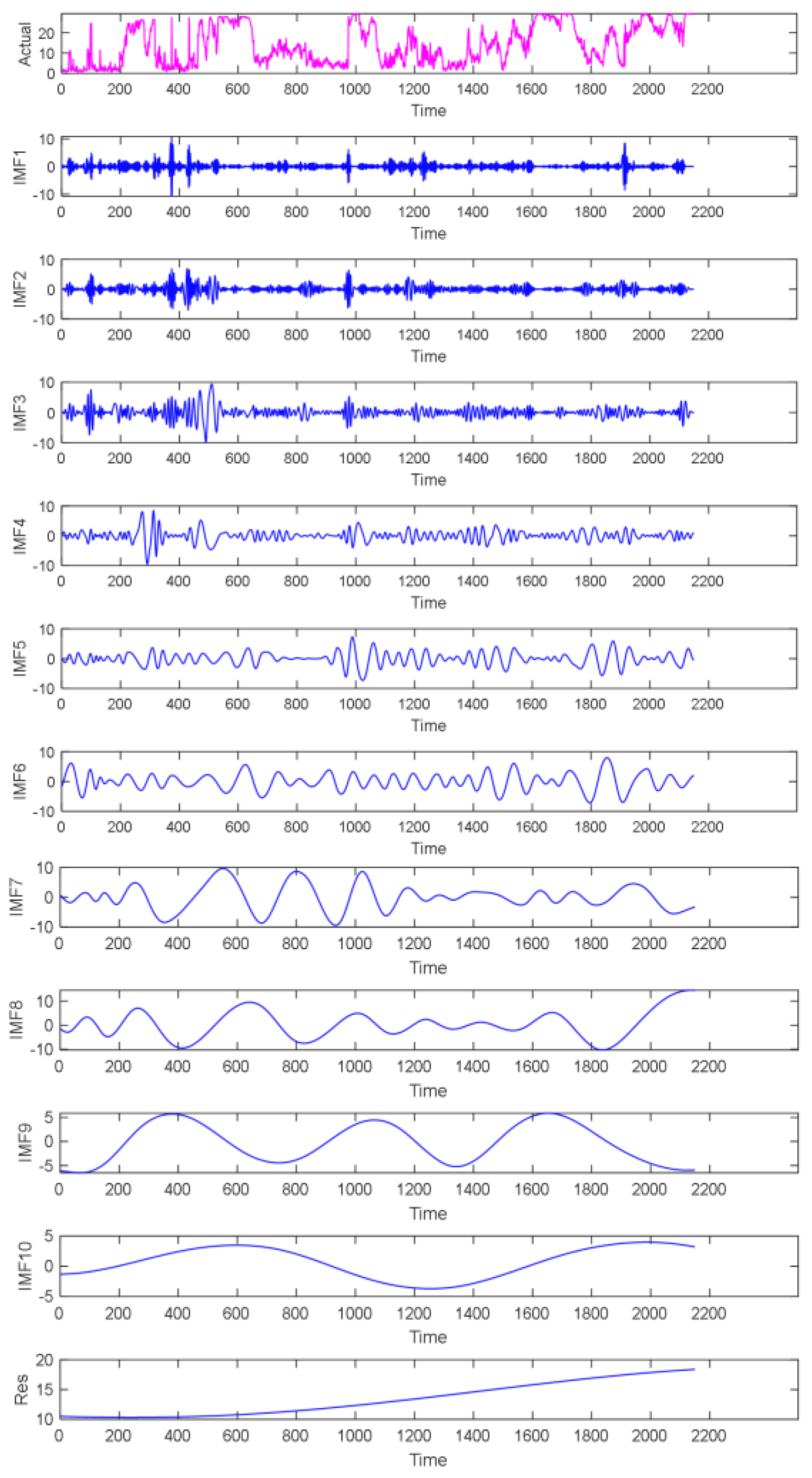
To further reduce the nonlinearity and strong volatility characteristics of the WP signal and enhance the forecasting precision, the EMD algorithm was first used to decompose the preprocessed SCADA data and then perform related calculations. The EMD decomposition results of the original WP data are shown in Figure 5. A total of 10 IMF components and 1 remaining component were decomposed, and they are plotted in blue. Figure 5 shows that the time characteristic scale of the eigenmode function component increased from IMF1 to IMF10, and the frequency changed from high to low.

Figure 5. Diagram of original WP data and its EMD decomposition.

3.3. Parameters Setting

In the present study, PSO-RBF and PSO-SVM models were established, and algorithms such as PSO, BES, and MBES were used to optimize the hyper-parameters of the LSTM. The relevant parameter values are shown in Table 7.

Table 7. The parameter values of PSO-RBF, PSO-SVM, PSO-LSTM, BES-LSTM, and MBES-LSTM.

Model Name	Parameter Name	Parameter Value
PSO-RBF	iterations N	100
	population P	10
	V1	3
	V2	3
	W	0.6
	b	[0.585,0.3050,0.969]
	c	[0.748,0.278,−3] [1.448,−0.227,3]
	w	[1,−1,1]
PSO-SVM	iterations N	100
	population P	10
	V1	2
	V2	2
	W	0.9
	C	87
	g	0.02
PSO-LSTM	iterations N	30
	population P	8
	C1	4
	C2	4
	W	0.9
	lower board lb	[1,1,1,0.001]
	upper board ub	[100,100,100,0.01]
BES-LSTM	iterations N	30
	population P	8
	lower board lb	[1,1,1,0.001]
	upper board ub	[100,100,100,0.01]
	α	2
MBES-LSTM	iterations N	30
	population P	8
	lower board lb	[1,1,1,0.001]
	upper board ub	[100,100,100,0.01]
	α	${\alpha }_c=exp\left(\frac{T-t}{T}\right)-1$

3.4. Evaluation Indicators

To better assess the performance of the MBES-LSTM forecasting model, RMSE, MAE, MAPE, COV, CC, TIC, EC, and r² were used in the present study. The specific expressions are as follows:

(1) The root mean square error (RMSE) indicates the deviation between the predicted and actual values.

$$RMSE=\sqrt{\frac{1}{N}{{\displaystyle \sum _{t=1}^N\left(u_{actual}^t-u_{predict}^t\right)}}^2}$$

(20)

(2) The mean absolute error (MAE) reflects the actual situation of the errors, and this value also becomes larger when the error is large.

$$MAE=\frac{1}{N}{\displaystyle \sum _{t=1}^N\left|u_{actual}^t-u_{predict}^t\right|}$$

(21)

(3) The mean absolute percentile error (MAPE) is used to the measure forecast accuracy. Smaller MAPE values indicate that the model is more accurate in predicting

$$MAPE=\frac{1}{N}{\displaystyle \sum _{t=1}^N\left|\frac{u_{actual}^t-u_{predict}^t}{u_{actual}^t}\right|}$$

(22)

(4) The coefficient of variance (COV) [24] reflects the degree of discretization of the data, with a larger value indicating a higher degree of data scattering.

$$COV=\frac{RMSE}{u_{actmean}}\times 100\%$$

(23)

(5) The correlation coefficient (CC) represents the relationship between the actual and predicted values. This value is close to 1 when the actual data is strongly correlated with the predicted data.

$$CC=\frac{N{\displaystyle \sum _{t=1}^N\left(u_{actual}^t\times u_{predict}^t\right)-\left({\displaystyle \sum _{t=1}^N{u}_{actual}^t}\right)\left({\displaystyle \sum _{t=1}^N{u}_{predict}^t}\right)}}{\left[N\left({\displaystyle \sum _{t=1}^N{\left(u_{actual}^t\right)}^2}\right)-{\left({\displaystyle \sum _{t=1}^N{u}_{actual}^t}\right)}^2\right]\left[N\left({\displaystyle \sum _{t=1}^N{\left(u_{predict}^t\right)}^2}\right)-{\left({\displaystyle \sum _{t=1}^N{u}_{predict}^t}\right)}^2\right]}$$

(24)

(6) The Theil’s inequality coefficient (TIC) [25], with a value range between [0, 1]. The smaller the TIC value, the better the prediction accuracy of the model.

$$TIC=\frac{\sqrt{\frac{1}{N}{{\displaystyle \sum _{t=1}^N\left(u_{actual}^t-u_{predict}^t\right)}}^2}}{\sqrt{\frac{1}{N}{{\displaystyle \sum _{t=1}^N\left(u_{actual}^t\right)}}^2}+\sqrt{\frac{1}{N}{{\displaystyle \sum _{t=1}^N\left(u_{predict}^t\right)}}^2}}$$

(25)

(7) The efficiency coefficient (EC) [26] is generally used to verify the goodness of fit of the model’s prediction results, and if the EC is close to 1, the prediction quality of the model is good.

$$EC=1-\frac{\frac{1}{N}{{\displaystyle \sum _{t=1}^N\left(u_{actual}^t-u_{predict}^t\right)}}^2}{\frac{1}{N}{{\displaystyle \sum _{t=1}^N\left(u_{actual}^t-u_{actmean}^{}\right)}}^2}$$

(26)

(8) The coefficient of determination r² (r²) estimates the combined dispersion against the single dispersion of the observed and predicted series.

$$r^2={\left(\frac{{\displaystyle \sum _{t=1}^N\left[\left(u_{actual}^t-u_{actmean}^{}\right)\times \left(u_{predict}^t-u_{premean}^{}\right)\right]}}{\sqrt{{{\displaystyle \sum _{t=1}^N\left(u_{actual}^t-u_{actmean}^{}\right)}}^2}\times \sqrt{{{\displaystyle \sum _{t=1}^N\left(u_{predict}^t-u_{premean}^{}\right)}}^2}}\right)}^2$$

(27)

where $u_{actual}^t$ represents the WP observation value at time t; $u_{predict}^t$ is the WP forecast value at time t; $u_{actmean}$ is the average WP observation; $u_{premean}$ is the average WP forecast; and N is the number of samples in the $u{}^t$ sequence.

4. Experimental Results and Discussion

In WP forecasting, the setting of related parameters directly affects the forecasting precision of the LSTM network. In the present study, the PSO, BES, and MBES algorithms were used to optimize the hyper-parameters such as $T_{iter}$, $L_R$, $L_1$, and $L_2$. The LSTM-related parameter values and calculated errors in each IMF decomposition are shown in Table 8.

Table 8. The LSTM hyper-parameters value and errors based on PSO, BES, and MBES.

Model	EMD	iter	LR	L1	L2	RMSE	MAPE
PSO-LSTM	IMF1	43	0.0050	7	91	0.7891	0.5498
	IMF2	95	0.0058	93	25	0.2829	0.2046
	IMF3	52	0.0079	86	65	0.1432	0.1125
	IMF4	88	0.0086	64	34	0.2111	0.1589
	IMF5	69	0.0048	20	62	0.1020	0.0784
	IMF6	70	0.0039	66	32	0.2686	0.1637
	IMF7	48	0.0063	38	10	0.1351	0.0854
	IMF8	72	0.0064	70	40	0.5410	0.2376
	IMF9	92	0.0093	34	93	0.3567	0.1505
	IMF10	86	0.0059	61	95	0.3453	0.2160
	Res	33	0.0074	11	67	0.5596	0.4408
BES-LSTM	IMF1	24	0.0087	71	20	0.7884	0.5453
	IMF2	50	0.01	100	44	0.2782	0.2001
	IMF3	49	0.0097	97	97	0.1266	0.0964
	IMF4	23	0.0098	54	78	0.1097	0.0879
	IMF5	50	0.01	100	94	0.1098	0.0810
	IMF6	41	0.0082	4	32	0.1945	0.0923
	IMF7	28	0.0032	52	12	0.1179	0.0710
	IMF8	43	0.0011	96	51	0.4455	0.2112
	IMF9	38	0.01	100	100	0.3035	0.1352
	IMF10	50	0.01	56	100	0.3198	0.1292
	Res	48	0.0057	92	14	0.3602	0.1307
MBES-LSTM	IMF1	17	0.0058	63	27	0.7909	0.5522
	IMF2	90	0.0070	96	89	0.2829	0.2046
	IMF3	87	0.0062	89	82	0.1145	0.0838
	IMF4	85	0.0067	51	83	0.0995	0.0751
	IMF5	80	0.0052	43	23	0.1020	0.0784
	IMF6	67	0.0063	43	51	0.1856	0.0641
	IMF7	26	0.0040	56	41	0.1006	0.0685
	IMF8	87	0.0088	29	43	0.3528	0.1775
	IMF9	71	0.0093	34	93	0.2875	0.1220
	IMF10	86	0.0059	61	95	0.2804	0.1193
	Res	67	0.0092	54	45	0.3492	0.0980

Table 9 indicates the Loss and RMSE of the LSTM, PSO-LSTM, BES-LSTM, and MBES-LSTM models in the training set and the testing set. An observation can be made that the MBES-LSTM model trends towards small Loss and RMSE value in the training set and the testing set.

Table 9. Forecasting errors of LSTM, PSO-LSTM, BES-LSTM, and MBES-LSTM models.

Model Name	Training Set		Testing Set
	RMSE	Loss	RMSE	Loss
LSTM	0.1926	0.0246	2.0632	1.3091
PSO-LSTM	0.1724	0.0148	1.7649	1.2462
BES-LSTM	0.1613	0.0111	1.7079	1.1709
MBES-LSTM	0.1451	0.0114	1.6158	1.0945

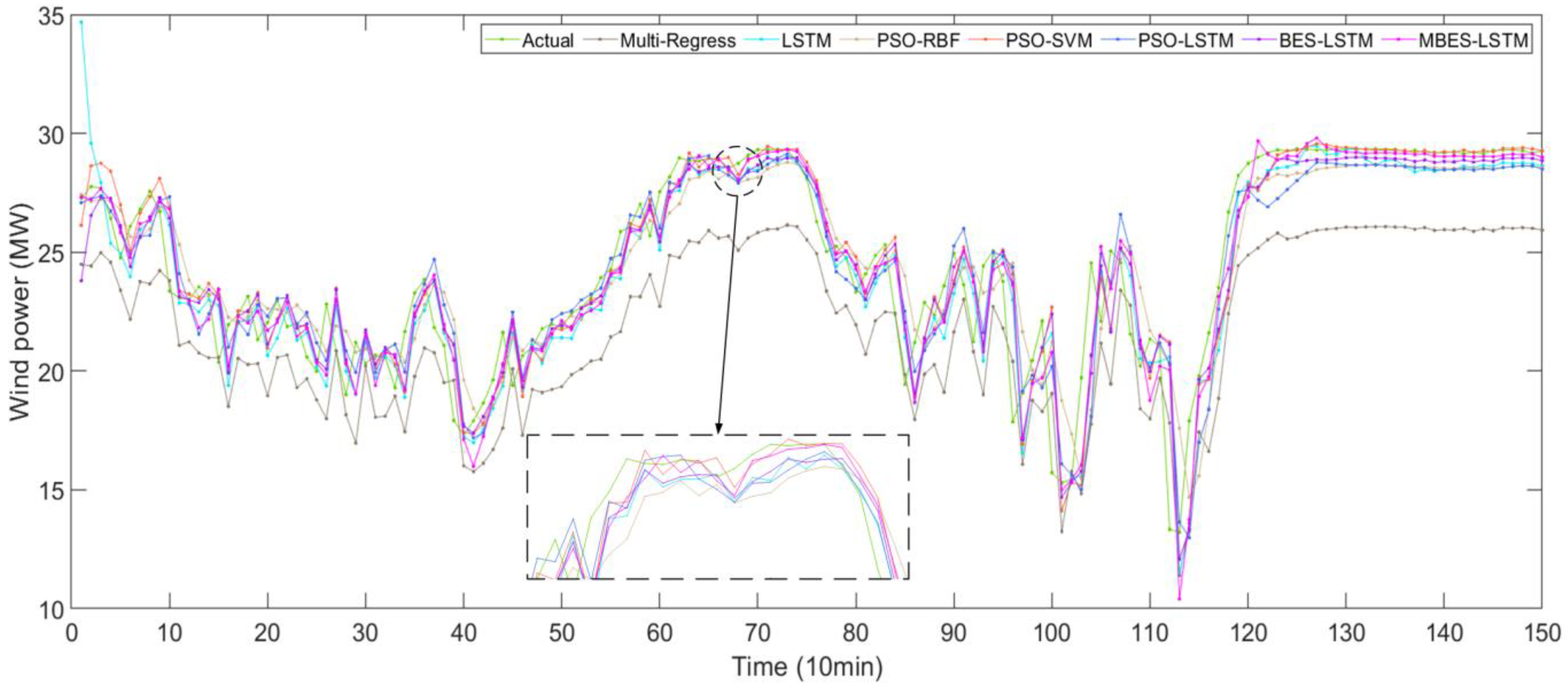
To further reflect the advantages of the MBES-LSTM forecasting model, some models were contrasted with other models such as the Multi-Regress, LSTM, PSO-RBF, PSO-SVM, PSO-LSTM, and BES-LSTM models. Figure 6 shows a comparison diagram of the direct forecasting results of the models. It can be noted from Figure 6 that the prediction line of the multi-regress model was far away from the actual line, indicating that the prediction results were poor, while the prediction lines of other models were near the actual lines.

Figure 6. The forecasting results of different models.

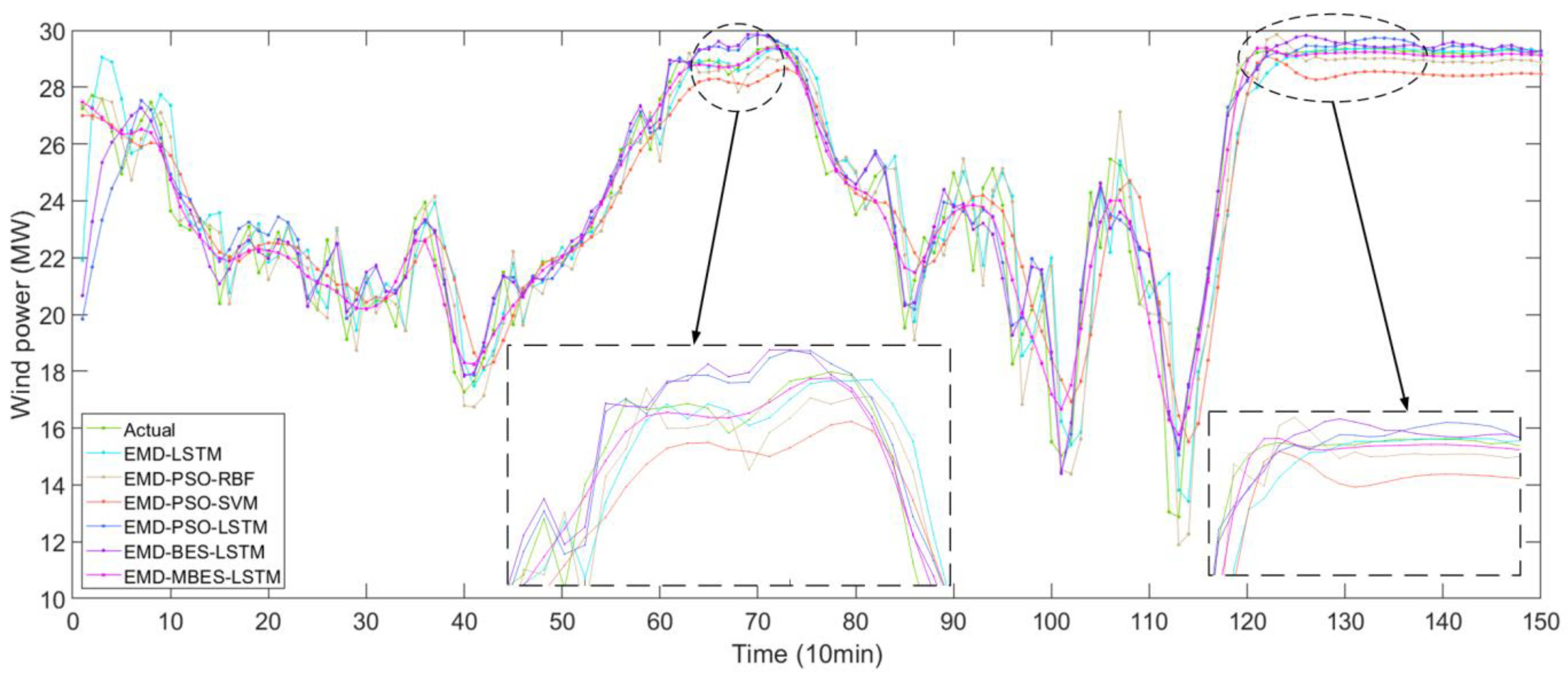
Figure 7 shows the forecasting results of different models based on the EMD algorithm.

Figure 7. The forecasting results of different models based on EMD.

In Figure 6 and Figure 7, the solid green line represent the actual values, while the remaining six colored lines represent the forecasted values. The closer their location to the green line, the higher the forecasting accuracy of the models. An observation can be made that the forecasting value line of the MBES-LSTM model was closer to the green line, which indicates that the forecasting precision of MBES-LSTM was the highest.

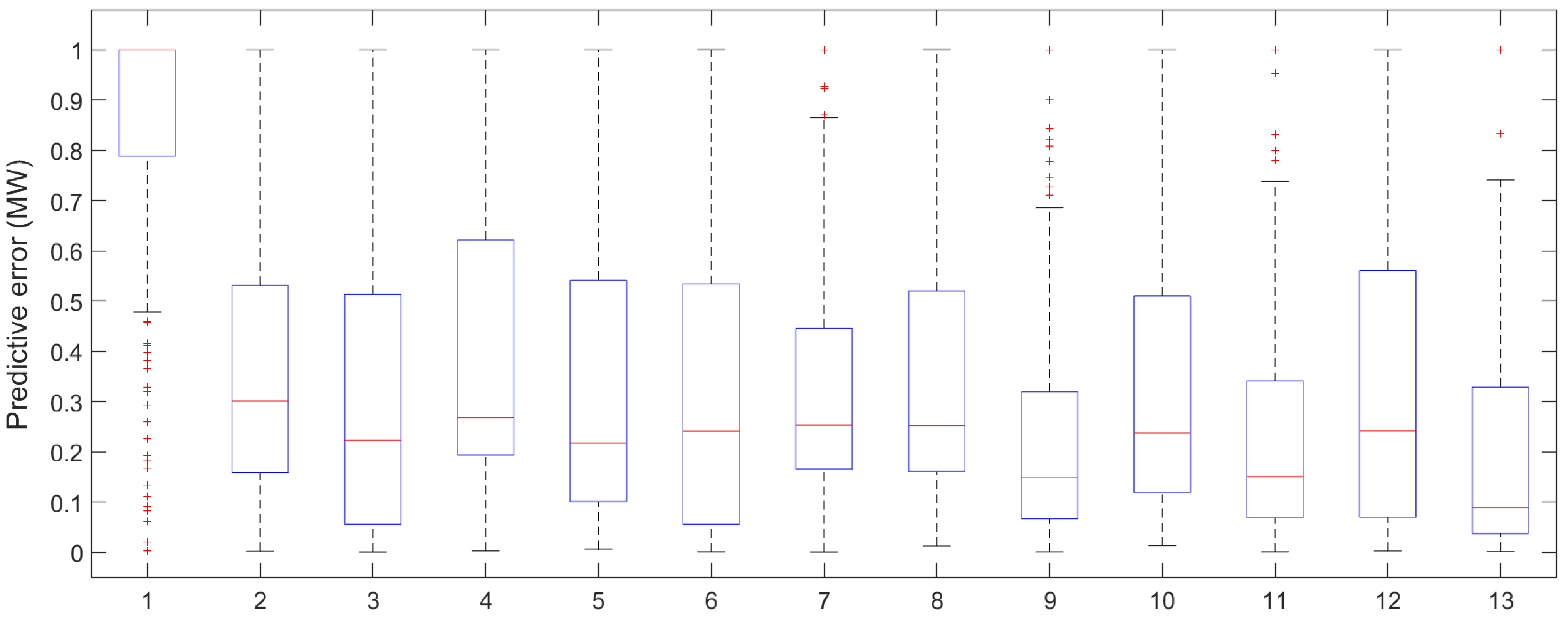
In order to more intuitively reflect the size of the forecasting error, a box-plot was drawn to graphically present the forecasting error, as shown in Figure 8. According to the box-plot, the MBES-LSTM model based on EMD showed less errors.

Figure 8. The box-plot of forecasting errors of the different models (1, Multi-Regress; 2, LSTM; 3, EMD-LSTM; 4, PSO-RBF; 5, EMD-PSO-RBF; 6, PSO-SVM; 7, EMD-PSO-SVM; 8, PSO-LSTM; 9, EMD-PSO-LSTM; 10, BES-LSTM; 11, EMD-BES-LSTM; 12, MBES-LSTM; 13, EMD-MBES-LSTM).

Formulas (20)–(27) were used to calculate the relevant evaluation indicators of each forecasting model. The calculation results are shown in Table 10, according to which proposed EMD-MBES-LSTM model had the optimal forecasting performance, exhibiting the highest performance indexes.

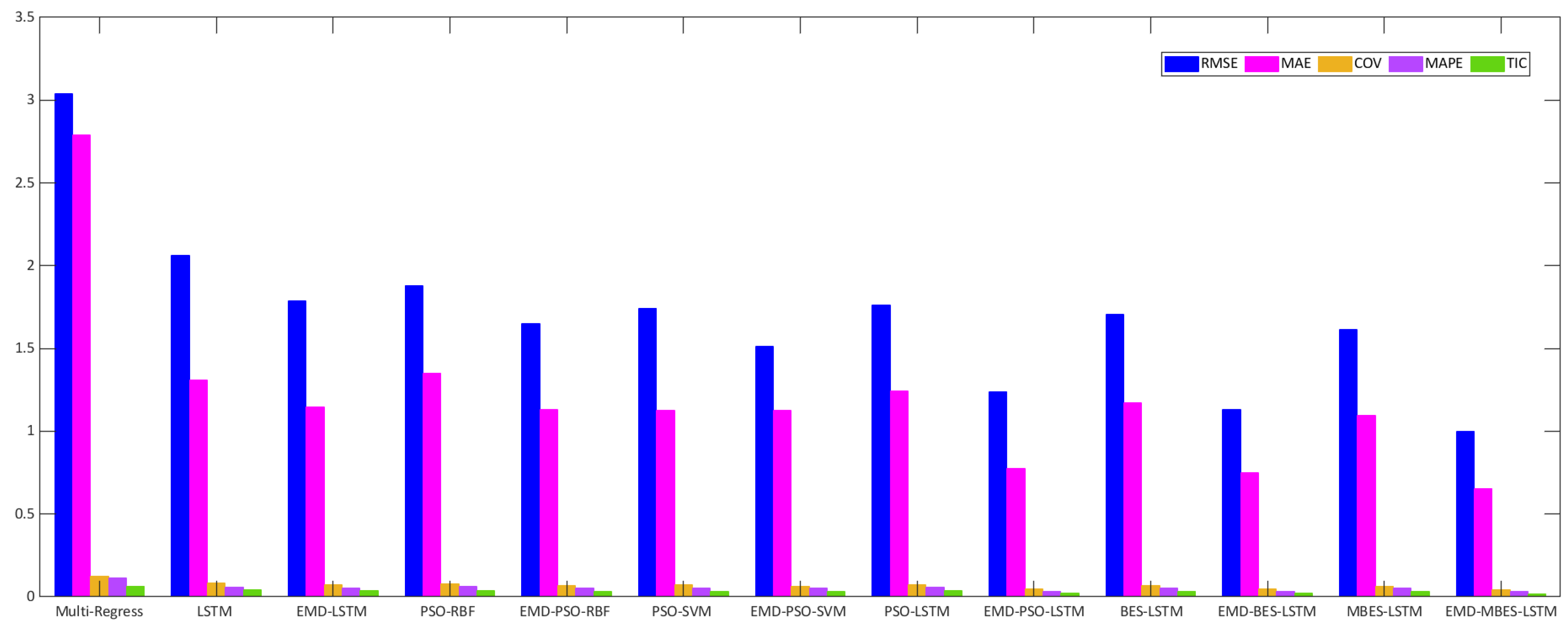
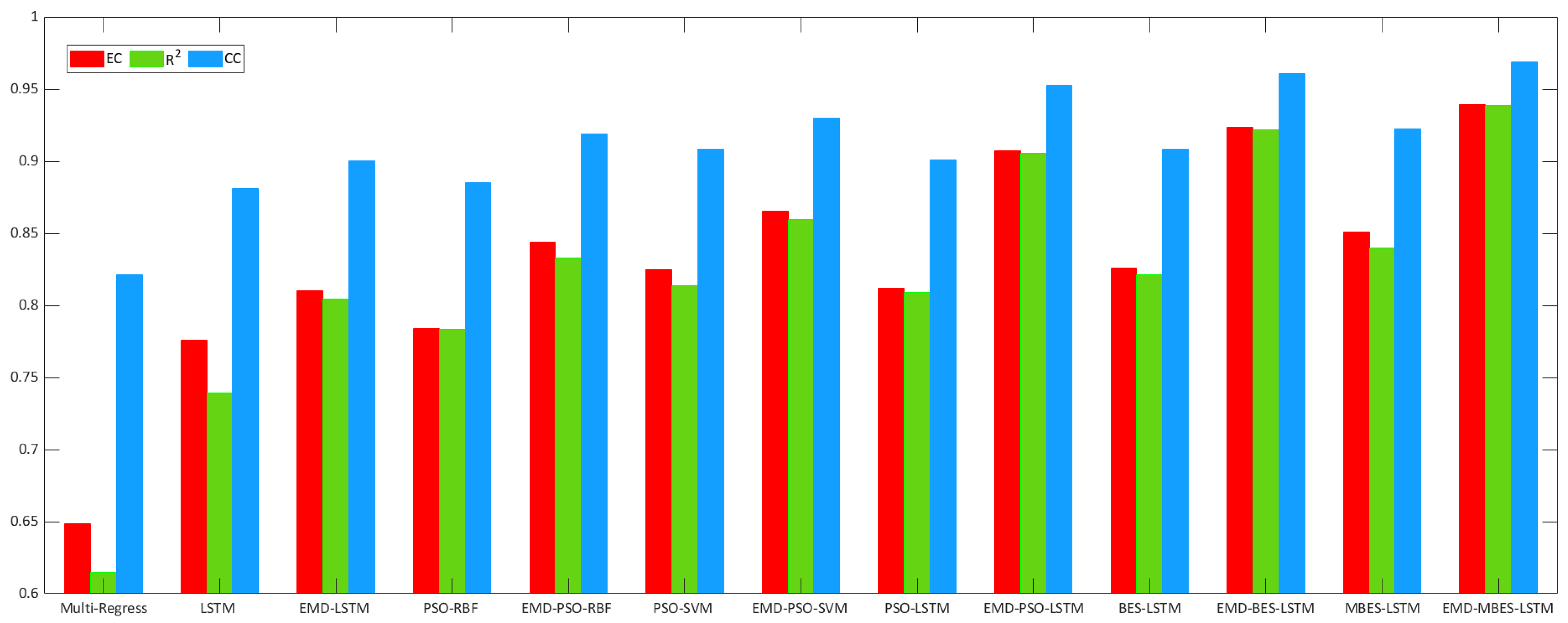
Table 10. Comparison of evaluation metrics.

Forecasting Models	RMSE	MAE	COV	MAPE	TIC	NSE	R2	CC
Multi-Regress	3.0374	2.7887	0.1243	0.1143	0.0648	0.6486	0.6150	0.8212
LSTM	2.0632	1.3091	0.0845	0.0592	0.0419	0.7761	0.7393	0.8810
EMD-LSTM	1.7881	1.1484	0.0732	0.0539	0.0360	0.8103	0.8042	0.9001
PSO-RBF	1.8815	1.3516	0.0770	0.0629	0.0381	0.7839	0.7832	0.8854
EMD-PSO-RBF	1.6514	1.1329	0.0676	0.0532	0.0334	0.8441	0.8330	0.9188
PSO-SVM	1.7441	1.1274	0.0714	0.0533	0.0352	0.8250	0.8137	0.9083
EMD-PSO-SVM	1.5146	1.1253	0.0620	0.0513	0.0307	0.8654	0.8595	0.9302
PSO-LSTM	1.7649	1.2462	0.0722	0.0568	0.0358	0.8117	0.8092	0.9009
EMD-PSO-LSTM	1.7649	1.2462	0.0722	0.0568	0.0358	0.8117	0.8092	0.9009
BES-LSTM	1.7079	1.1709	0.0699	0.0542	0.0346	0.8257	0.8213	0.9087
EMD-BES-LSTM	1.1310	0.7508	0.0463	0.0337	0.0228	0.9234	0.9217	0.9609
MBES-LSTM	1.6158	1.0945	0.0661	0.0517	0.0327	0.8506	0.8401	0.9223
EMD-MBES-LSTM	1.0009	0.6550	0.0410	0.0310	0.0202	0.9391	0.9386	0.9691

Figure 9 and Figure 10 describe the relevant evaluation index histograms. In Figure 9, the height of the blue column represents the RMSE of the Multi-Regress, LSTM, PSO-RBF, PSO-SVM, PSO-LSTM, BES-LSTM, and MBES-LSTM forecasting models; the height of the magenta column represents the MAE of every model; the height of the green column represents the TIC. In Figure 10, the height of the red column represents the EC, and the height of the green column represents the r² of each model. From Figure 9 and Figure 10, an observation can be made that the MBES-LSTM model described in the present study showed the minimum evaluation error and highest evaluation coefficient, regardless of which evaluation standard was used.

Figure 9. Evaluation error of different forecasting models.

Figure 10. Evaluation coefficient results of different forecasting models.

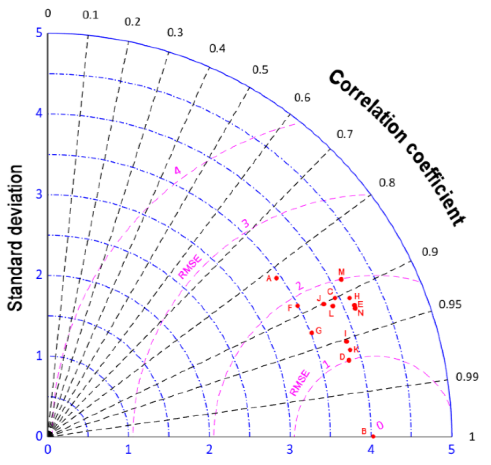
A Taylor diagram of the forecasting models is shown in Figure 11. In Figure 11, point D is closest to point B, indicating that point D had the best performance metrics. Specifically, the MBES-LSTM model based on EMD had the optimal predictive performance.

Figure 11. The Taylor diagram of the forecasting results (A: Multi-Regress; B: Actual; C: EMD-LSTM; D: EMD-MBES-LSTM; E: EMD-PSO-RBFF; F: PSO-RB; G: EMD-PSO-SVM; H: PSO-SVM; I: EMD-PSO-LSTM; J: PSO-LSTM; K: EMD-BES-LSTM; L: BES-LSTM; M: LSTM; N: MBES-LSTM).

The MBES-LSTM model based on EMD has many advantages. Compared with the other models, there was a significant improvement in the forecasting accuracy in terms of WP forecasting. The MBES-LSTM model can be summarized as follows:

(1) The EMD algorithm was a significant factor in data preprocessing, and it significantly improved the forecasting accuracy. As can be seen from Figure 6 and Figure 7 and Table 10, after EMD decomposition on LSTM, RMSE decreased by about 0.2751, MAE decreased by about 0.1607, and r² increased by about 0.0649.

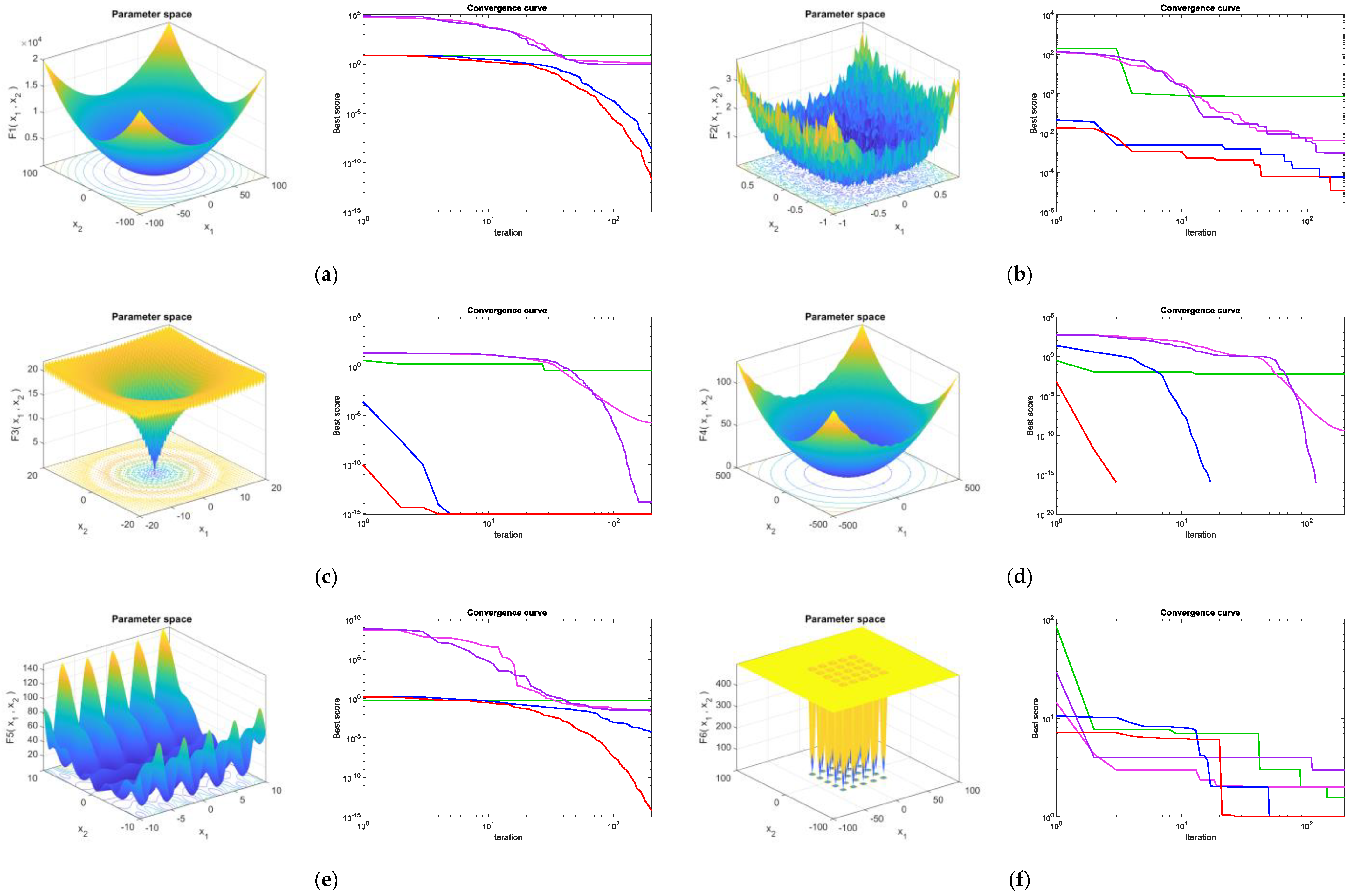
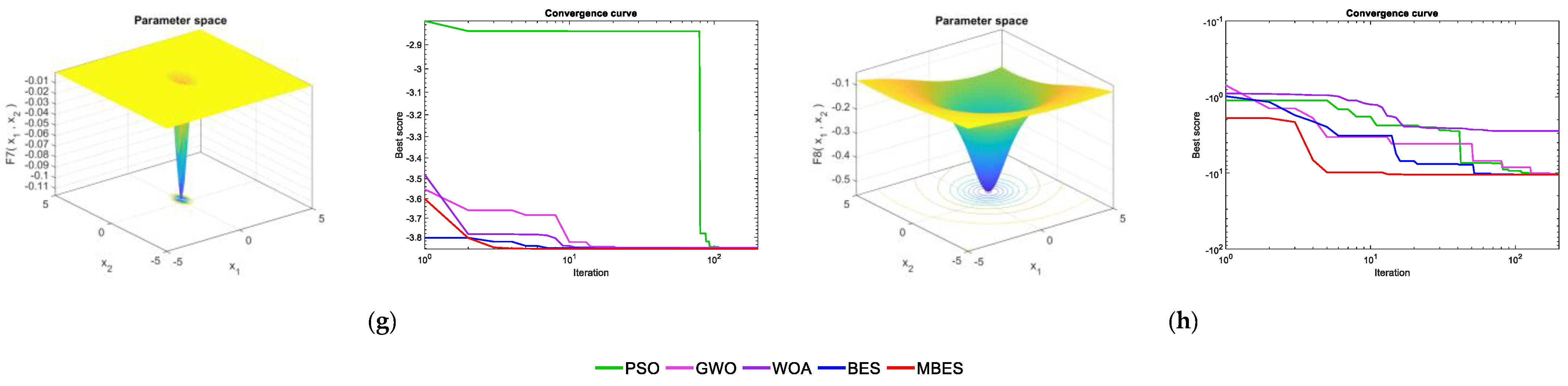
(2) The proposed algorithm was evaluated through several different benchmark functions and was applied in the parameter estimation of LSTM. As can be seen from Table 9 and Table 10, compared with the standard bald eagle algorithm, the modified bald eagle algorithm had a positive effect on LSTM hyper-parameter optimization. After optimizing the related parameters of LSTM with the modified bald eagle algorithm, RMSE decreased by about 0.0922, MAE decreased by about 0.0764, and r² increased by about 0.0188.

5. Conclusions

Accurate forecasting of WP is integral for the safe dispatch of power systems and the operation management of wind farms. In the field of WP forecasting, LSTM is a commonly used in-depth learning algorithm. With the aim of solving the problem that the improper selection of LSTM related parameters $\{T_{iter},L_R,L_1^{},L_2^{}\}$ may adversely affect the forecasting results of the LSTM, an MBES-LSTM WP short-term forecasting model was established in the present study.

(1) In the selection phase, the improvement of parameters is based on creating varied values for the learning parameter in each iteration, which helps to enhance the exploration of the MBES algorithm.

(2) The MBES algorithm was adopted to optimize the relevant parameters $\{T_{iter},L_R,L_1^{},L_2^{}\}$ of the LSTM to form the MBES-LSTM model. In the WP forecasting test on the wind farm, the forecasting accuracy rate was better than that of the PSO-RBF, PSO-SVM, LSTM, PSO-LSTM, and BES-LSTM models.

Only historical WP data are used in the MBES-LSTM forecasting model. The WP is constantly affected by external factors, such as the wind direction, landforms, humidity, air temperature, and atmospheric pressure. Such factors will lead to rapidness, high nonlinearity, and uncertainty of WP changes, and thus, should be considered reasonable when establishing a multi-input forecasting model. In this way, the accuracy of WP forecasting can be further improved, which is also indicated for future study.

References

- Gu, B.; Zhang, T.; Meng, H.; Zhang, J. Short-term forecasting and uncertainty analysis of wind power based on long short-term memory, cloud model and non-parametric kernel density estimation. Renew. Energy 2021, 164, 687–708. [Google Scholar] [CrossRef]
- Xue, F.; Duan, H.; Xu, C.; Han, X.; Shangguan, Y.; Li, T.; Fen, Z. Research on the Power Capture and Wake Characteristics of a Wind Turbine Based on a Modified Actuator Line Model. Energies 2022, 15, 282. [Google Scholar] [CrossRef]
- Gu, C.; Li, H. Review on Deep Learning Research and Applications in Wind and Wave Energy. Energies 2022, 15, 1510. [Google Scholar] [CrossRef]
- WWEA. Worldwide Wind Capacity Reaches 744 Gigawatts–An Unprecedented 93 Gigawatts Added in 2020. Available online: https://wwindea.org/worldwide-wind-capacity-reaches-744-gigawatts/ (accessed on 24 March 2021).
- Donadio, L.; Fang, J.; Porté-Agel, F. Numerical Weather Prediction and Artificial Neural Network Coupling for Wind Energy Forecast. Energies 2021, 14, 338. [Google Scholar] [CrossRef]
- Pichault, M.; Vincent, C.; Skidmore, G.; Monty, J. Short-Term Wind Power Forecasting at the Wind Farm Scale Using Long-Range Doppler LiDAR. Energies 2021, 14, 2663. [Google Scholar] [CrossRef]
- Landberg, L. A mathematical look at a physical power prediction model. Wind Energy 1998, 1, 23–28. [Google Scholar] [CrossRef]
- Lydia, M.; Kumar, S.S.; Selvakumar, A.I.; Kumar, G.E.P. Linear and non-linear autoregressive models for short-term wind speed forecasting. Energy Convers. Manag. 2016, 112, 115–124. [Google Scholar] [CrossRef]
- Han, Q.; Meng, F.; Hu, T.; Chu, F. Non-parametric hybrid models for wind speed forecasting. Energy Convers. Manag. 2017, 148, 554–568. [Google Scholar] [CrossRef]
- Lodge, A.; Yu, X.H. Short Term Wind Speed Prediction Using Artificial Neural Networks. In Proceedings of the 2014 4th IEEE International Conference on Information Science and Technology, Shenzhen, China, 26–28 April 2014; pp. 539–542. [Google Scholar] [CrossRef]
- Kalogirou, S.; Neocleous, C.; Pashiardis, S.; Schizas, C.N. Wind speed prediction using artificial neural networks. In Proceedings of the European Symposium on Intelligent Techniques, Crete, Greece, 3–4 June 1999. [Google Scholar]
- Lorenzo, J.; Mendez, J.; Castrillon, M.; Hernandez, D. Short-Term Wind Power Forecast Based on Cluster Analysis and Artificial Neural Networks. In Proceedings of the 11th International Work-Conference on Artificial Neural Networks (Advances in Computational Intelligence, IWANN 2011, Pt I), Torremolinos-Málaga, Spain, 8–10 June 2011; Cabestany, J., Rojas, I., Joya, G., Eds.; Springer: Berlin/Heidelberg, Germany; Volume 6691, pp. 191–198. [Google Scholar]
- An, G.; Jiang, Z.; Cao, X.; Liang, Y.; Zhao, Y.; Li, Z.; Dong, W.; Sun, H. Short-Term Wind Power Prediction Based on Particle Swarm Optimization-Extreme Learning Machine Model Combined with Adaboost Algorithm. IEEE Access 2021, 9, 94040–94052. [Google Scholar] [CrossRef]
- Hur, S. Short-term wind speed prediction using Extended Kalman filter and machine learning. Energy Rep. 2021, 7, 1046–1054. [Google Scholar] [CrossRef]
- Elsheikh, A.H.; Sharshir, S.W.; Abd Elaziz, M.; Kabeel, A.E.; Guilan, W.; Haiou, Z. Modeling of solar energy systems using artificial neural network: A comprehensive review. Sol. Energy 2019, 180, 622–639. [Google Scholar] [CrossRef]
- Huang, D.; Gong, R.; Gong, S. Prediction of Wind Power by Chaos and BP Artificial Neural Networks Approach Based on Genetic Algorithm. J. Electr. Eng. Technol. 2015, 10, 41–46. [Google Scholar] [CrossRef] [Green Version]
- Guo, P.; Qi, Z.; Huang, W. Short-term wind power prediction based on genetic algorithm to optimize RBF neural network. In Proceedings of the 2016 Chinese Control and Decision Conference (CCDC), Yinchuan, China, 28–30 May 2016; pp. 1220–1223. [Google Scholar]
- Peng, X.; Li, Y.; Dong, L.; Cheng, K.; Wang, H.; Xu, Q.; Wang, B.; Liu, C.; Che, J.; Yang, F.; et al. Short-Term Wind Power Prediction Based on Wavelet Feature Arrangement and Convolutional Neural Networks Deep Learning. IEEE Trans. Ind. Appl. 2021, 57, 6375–6384. [Google Scholar] [CrossRef]
- Lin, Z.; Liu, X.; Collu, M. Wind power prediction based on high-frequency SCADA data along with isolation forest and deep learning neural networks. Int. J. Electr. Power Energy Syst. 2020, 118, 105835. [Google Scholar] [CrossRef]
- Chen, X.; Zhang, X.; Dong, M.; Huang, L.; Guo, Y.; He, S. Deep Learning-Based Prediction of Wind Power for Multi-turbines in a Wind Farm. Front. Energy Res. 2021, 9, 403. [Google Scholar] [CrossRef]
- Hochreiter, S.; Schmidhuber, J. Long Short-Term Memory. Neural Comput. 1997, 9, 1735–1780. [Google Scholar] [CrossRef]
- Alsattar, H.A.; Zaidan, A.A.; Zaidan, B.B. Novel meta-heuristic bald eagle search optimisation algorithm. Artif. Intell. Rev. 2020, 53, 2237–2264. [Google Scholar] [CrossRef]
- Hansen, A.J. Fighting Behavior in Bald Eagles: A Test of Game Theory. Ecology 1986, 67, 787–797. [Google Scholar] [CrossRef]
- Elsheikh, A.H.; Panchal, H.; Ahmadein, M.; Mosleh, A.O.; Sadasivuni, K.K.; Alsaleh, N.A. Productivity forecasting of solar distiller integrated with evacuated tubes and external condenser using artificial intelligence model and moth-flame optimizer. Case Stud. Therm. Eng. 2021, 28, 101671. [Google Scholar] [CrossRef]
- Tian, Z.; Chen, H. A novel decomposition-ensemble prediction model for ultra-short-term wind speed. Energy Convers. Manag. 2021, 248, 114775. [Google Scholar] [CrossRef]
- Elsheikh, A.H.; Katekar, V.P.; Muskens, O.L.; Deshmukh, S.S.; Elaziz, M.A.; Dabour, S.M. Utilization of LSTM neural network for water production forecasting of a stepped solar still with a corrugated absorber plate. Process Saf. Environ. Prot. 2021, 148, 273–282. [Google Scholar] [CrossRef]
Publisher’s Note: MDPI stays neutral with regard to jurisdictional claims in published maps and institutional affiliations. |
© 2022 by the authors. Licensee MDPI, Basel, Switzerland. This article is an open access article distributed under the terms and conditions of the Creative Commons Attribution (CC BY) license (https://creativecommons.org/licenses/by/4.0/).