Dissolved Gas Analysis and Application of Artificial Intelligence Technique for Fault Diagnosis in Power Transformers: A South African Case Study

Abstract

In South Africa, the growing power demand, challenges of having idle infrastructure, and power delivery issues have become crucial problems. Reliability enhancement necessitates a life-cycle performance analysis of the electrical power transformers. To attain reliable operation and continuous electric power supply, methodical condition monitoring of the electrical power transformer is compulsory. Abrupt breakdown of the power transformer instigates grievous economic detriment in the context of the cost of the transformer and disturbance in the electrical energy supply. On the condition that the state of the transformer is appraised in advance, it can be superseded to reduced loading conditions as an alternative to unexpected failure. Dissolved gas analysis (DGA) nowadays has become a customary method for diagnosing transformer faults. DGA provides the concentration level of various gases dissolved, and consequently, the nature of faults can be predicted subject to the concentration level of the gases. The prediction of fault class from DGA output has so far proven to be not holistically reliable when using conventional methods on account of the volatility of the DGA data in line with the rating and working conditions of the transformer. Several faults are unpredictable using the IEC gas ratio (IECGR) method, and an artificial neural network (ANN) has the hindrance of overfitting. Nonetheless, considering that transformer fault prediction is a classification problem, in this work, a unique classification algorithm is proposed. This applies a binary classification support vector machine (BCSVM). The classification precision is not reliant on the number of features of the input gases dataset. The results indicate that the proposed BCSVM furnishes improved results concerning IECGR and ANN methods traceable to its enhanced generalization capability and constructional risk-abatement principle.

1. Introduction

It is well documented that the power supply system is a composite network comprising several customers, i.e., residential, industrial, etc., operating at distinct voltage levels [1,2]. This distinct voltage level is facilitated using power and distribution transformers [2]. Consequently, the high degree of operational reliability and lucrative operation of the electrical transformers and, thereby, the power system are of considerable engineering significance. It is recognized that the performance and planned life span of a transformer is assignable to the decomposition of the dielectric system [3]. Moreover, this chain of events requires efficacious condition-monitoring procedures and diagnostic tools. For this reason, condition monitoring of dielectric oil and cellulosic paper insulation is an absolute priority to achieve a planned operational lifetime and to evade destructive failures of electrical transformers. Dissolved gas analysis (DGA) is a robust and generally acknowledged diagnostic tool in the transformer manufacturing industry. This is because DGA has the potential to divulge the electrical and thermal stresses predominating with transformer dielectric oil and cellulosic paper insulation. Prospective examination approaches for DGA fault diagnosis are reported in [4]. By and large, DGA fault diagnostic methods demonstrate high equivocation in examining the fault gases, given the nonlinear comportment of the fault gases and various problems with DGA fault diagnosis methods. The production of dissolved gases has a nonsequential connection with transformer duration of operation and insulation aging indicators, i.e., interfacial tension, furan, acidity, etc. [5]. This nonsequential comportment gives rise to intricacy in fault recognition when artificial intelligence algorithms are employed.

A handful of investigators have employed diverse intelligent methods comprising artificial neural networks (ANNs), fuzzy logic (FL), decision trees, etc. for diagnosing DGA faults [6,7]. As a result of the dubious accuracy and high equivocation in the classification of DGA faults, modern computational methods have been reported in recent years. These methods comprise machine learning algorithms and optimization algorithms. It is recognized that multidimensional and astronomical data samples are necessitated for training these algorithms to be efficacious. A handful of researchers have adopted these algorithms for diagnosing transformer DGA faults [8,9,10].

The current research contribution—This work presents a detailed investigation of transformer fault identification. Various open issues and research challenges in transformer fault identification using classical methods have been highlighted. The contributions of this research work are indicated as follows.

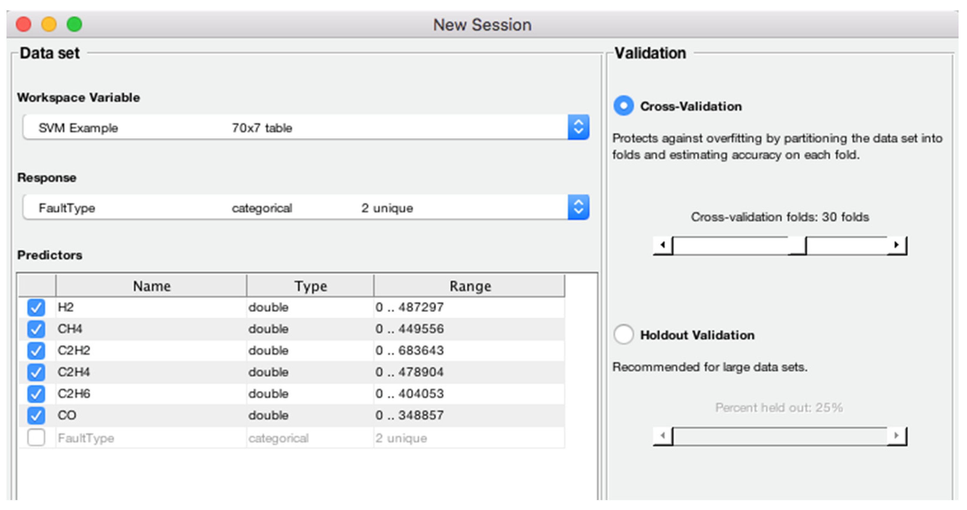
• A BCSVM is proposed for identifying a set of five transformer faults using 70% of the oil samples for training and 30% for training the proposed model, with 30-fold cross-validation applied in the training dataset. The proposed approach yields higher accuracy than ANN and the IEC method.
• The classification accuracy of the considered DGA samples is investigated by considering various machine learning algorithms, i.e., linear SVM, quadratic SVM, cubic SVM, fine Gaussian SVM, medium Gaussian SVM, and coarse Gaussian SVM, and comparing them in terms of accuracy (in percentage), prediction speed (objects/second) and training time (in seconds).
• A case study based on 14 transformer samples is presented using practical DGA data sets supplied by a South African manufacturer to comprehend fault classification proficiency in terms of accuracy of ANN and IEC methods and practical data versus the accuracy obtained in recent works.

The novelty of the current research—The fundamental purpose of this study is to ascertain a reliable transformer fault diagnosis approach using DGA and the application of the artificial intelligence technique for fault diagnosis in power transformers. Notwithstanding that numerous research workers have worked on the application of AI to diagnose transformer faults, as shown in Table 1, very seldom has research been published on fault diagnoses using BCSVM, particularly in transformer condition assessment. A reliable fault classification and prediction algorithm are crucial criteria for developing an efficient fault identification system. Three methods are considered a benchmark of the proposed method, and it was found that the IECGR method yields a “not detectable” response to some of the set of studied case studies and ANN yields a higher fault class than the actual fault in some oil samples due to model overfitting. However after the application of the proposed BCSVM algorithm, the “not detectable” samples were effectively identified.

Table 1. Summary of applicable works.

Ref. No	Year	Method	Summary
[11]	2020	SVM, ANN	The transformer condition is monitored daily and yields a precision of about 81.4% and 76%. The precision can be further increase.
[12]	2021	SVM, Bat algorithm	The study considers 160 data samples. which yield an accuracy of about 93.75%
[13]	2022	SVM, seagull optimization algorithm	180 field transformers are considered, and the proposed method yields an accuracy of 91.67%
[14]	2019	Least-square SVM, grey wolf optimization	MATLAB is utilized to classify transformer faults and yields an accuracy of 97.45%. The quantity of the data has not been highlighted.
[15,16]	2018	SVM, particle swarm optimization	Transformer faults are diagnosed using 118 databases adopted from the IEC TC 10 database and yield the highest accuracy of 85.71%

Many works compared the classical DGA methods in their investigations. Though there is similar work, in the current investigation, various machine learning (ML) algorithms, i.e., linear SVM, quadratic SVM, cubic SVM, fine Gaussian SVM, medium Gaussian SVM, and coarse Gaussian SVM, are compared in terms of accuracy (%), prediction Speed (objects/sec) and training time (sec). In the current study, the effect of the dissolved gas concentration levels is studied exclusively. This parameter is adopted for examining the performance of ML algorithms and two different diagnostic methods. From this investigation, it may be concluded that the proposed BCSVM algorithm is reliable in accurately diagnosing transformer faults using dissolved gas concentration levels in parts per million (ppm).

The manuscript organization—This research has been structured as follows. Section 2 presents the fundamental principle of the SVM algorithm and proposed BCSVM. Section 3 presents the results and discussion of the proposed algorithm for fault diagnosis of transformers. A corroboration of the proposed algorithm with the real sample datasets from local transformer companies in South Africa is presented. Lastly, Section 4 provides a conclusion of the manuscript.

2. Materials and Methods

2.1. Transformer Fault Classification Procedure

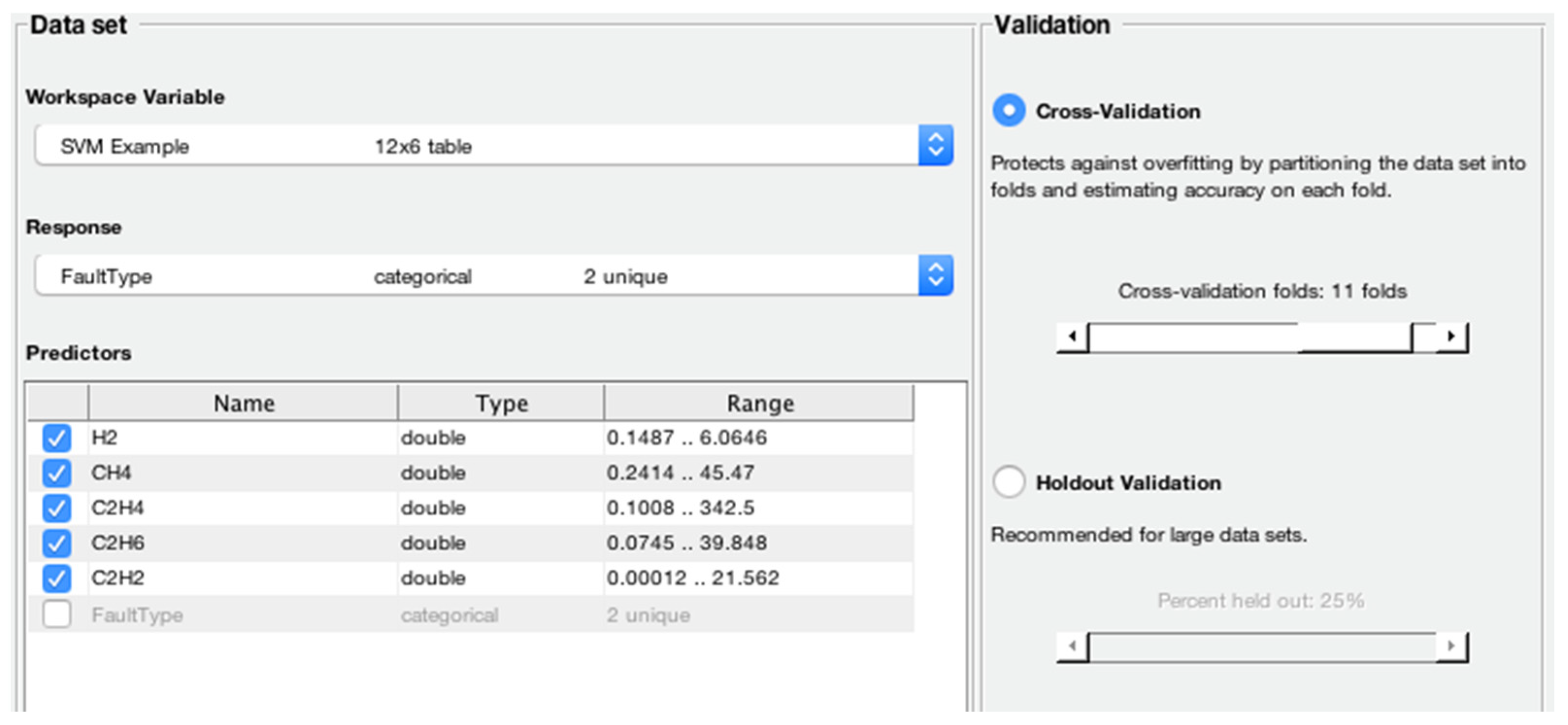
Transformer faults can be recognized in conformity with the dissolved gases proliferated attributable to the heating of the dielectric oil and the gases that are prevailing at diverse temperatures, i.e., hydrogen (${\mathrm{H}}_2$), carbon monoxide ($\mathrm{CO}$), methane (${\mathrm{CH}}_4$), ethane (${\mathrm{C}}_2{\mathrm{H}}_6$), ethylene (${\mathrm{C}}_2{\mathrm{H}}_4$), acetylene (${\mathrm{C}}_2{\mathrm{H}}_2$), and carbon dioxide (${\mathrm{CO}}_2$). Nevertheless, five gases, i.e., ${\mathrm{H}}_2$, ${\mathrm{CH}}_4$, ${\mathrm{C}}_2{\mathrm{H}}_4$, ${\mathrm{C}}_2{\mathrm{H}}_6$, and ${\mathrm{C}}_2{\mathrm{H}}_2$, are considered in this research in classifying transformer faults. A set of five transformer conditions, including no fault (NF), partial discharge (PD), and thermal fault conditions, are discerned.

2.2. The Fundamental Principle of the SVM Algorithm

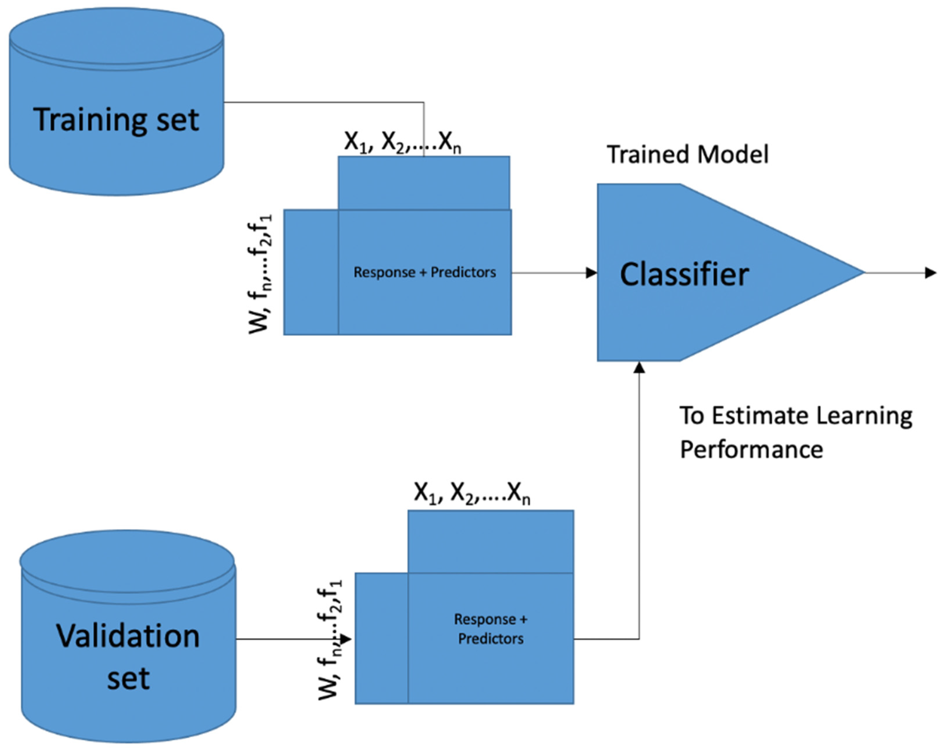
SVM is a vigorous supervised learning technique for developing a dataset classifier. SVM purports to establish a decision boundary among two classes of datasets that facilitate the forecasting of data labels from one or several feature vectors [11,12,13,14,15,16,17]. A decision boundary can be described as the area of a problem space whereupon the output dataset label of a classifier is equivocal. This decision boundary is referred to as the hyperplane, and it is positioned such that it is furthest from the nearest datasets from other classes. These nearest data points are so-called support vectors. The learning procedure of the SVM is illustrated in Figure 1. The SVM learns based on the training dataset entered. Then, the validation dataset is applied to determine the learning performance of the trained SVM algorithm. The trained SVM algorithm model is then applied to classifying samples of unknown test datasets.

Figure 1. The learning procedure of an SVM classifier.

Considering a tagged SVM training dataset, the latter can be expressed as follows in Equation (1).

$$\left(x_1, y_1\right),\dots \left(x_n, y_n\right),x_i\in R^d \mathrm{and} y\in \left(-1,+1\right)$$

(1)

Here,

$i—$Training compound

$x_i—$Feature vector (predictors)

$y_i—$Class label

An optimal hyperplane can therefore be expressed as follows in Equation (2).

$$w{x}^d+b=0$$

(2)

Here,

$w—$Weight vector

$x—$Input feature vector,

$b—$is the bias.

For all elements of the training dataset, the values of $w$ and $b$ must fulfill the conditions of the inequalities expressed in Equations (3) and (4).

$$w{x}_i{}^T+b\ge +1 \mathrm{if} y_i=1$$

(3)

$$w{x}_i{}^T+b\le -1 \mathrm{if} y_i=-1$$

(4)

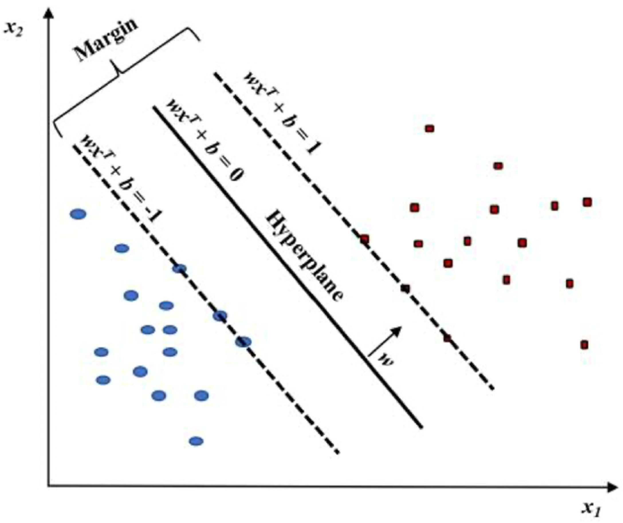
The purpose of training an SVM algorithm is to ascertain the $w$ and $b$ such that the hyperplane isolates the data points and makes the best use of the margin $\frac{1}{{||w||}^2}$. In Figure 2, the vectors $x_i$ with the property that $\left|y_i\right|$ $\left(w{x}_i{}^T+b\right)$ = 1 will be appellate as support vectors [12].

Figure 2. Linear SVM model classifying red vs. blue data points.

An alternative to a linear SVM classifier for the nonlinear application of the SVM is the kernel technique, which allows the modelling of higher dimensional and nonlinear models [11,12,13,14,15,16]. For a nonlinear problem, a kernel function can be employed to append supplemental dimensions to the coarse data and therefore create a linear problem in the eventuating higher dimensional space. In a nutshell, a kernel function, which is expressed as shown in Equation (5), can facilitate carrying computations rapidly, which would in other respects necessitate high dimensional space computations.

(5)

Here,

$K—$Kernel function

$x,y—n$ dimensional inputs

$f—$Map function of the input from $n$ dimensional to $m$ dimensional space

Indicate the dot product

Using kernel functions, the computation of the scalar product of data points in a higher dimensional space except specifically evaluating the mapping from the input space to the higher dimensional space can be conducted. In many instances, calculating the kernel is straightforward whereas in the high dimensional space, calculating the inner product of feature vectors is complex. The feature vector for even straightforward kernels can inflate in dimensions, and kernels such as the radial basis function (RBF) kernel can be expressed as follows in Equation (6).

$$K_{RBF}\left(x,y\right)=e^{\left(-\gamma {||x-y||}^2\right)}$$

(6)

The proportionate feature vector is incalculable dimensionally. Even so, calculating the kernel is nearly insignificant. Contingent on the essence of the problem, it is likely that one kernel can be a whole lot better than other kernels. An optimum kernel function can be chosen from an established set of kernels numerically in an extremely thorough and careful manner by applying cross-validation.

2.3. Proposed BCSVM Algorithm

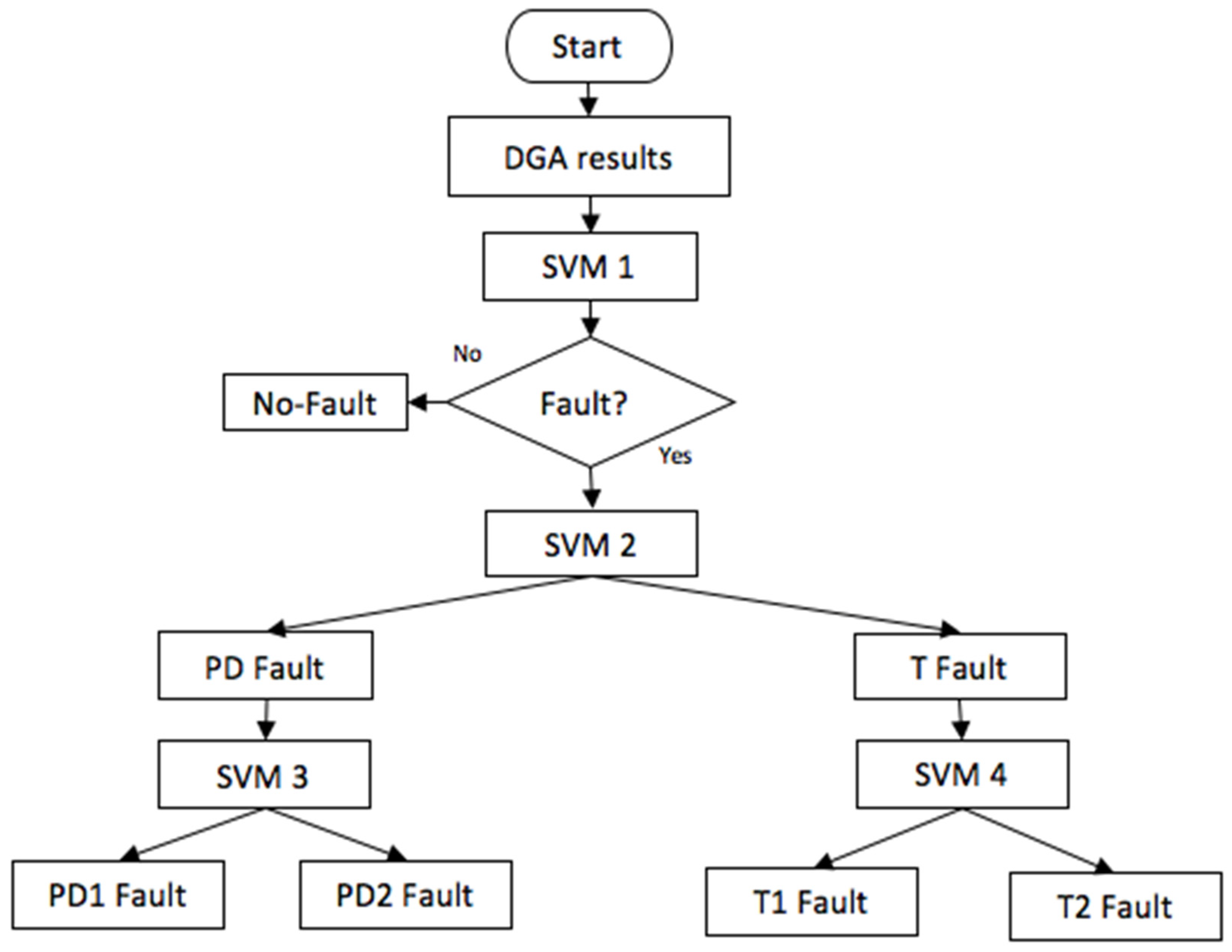
In the current study, DGA oil samples were obtained from mineral oil-immersed transformers in the field owned by different local independent power utilities. The comprehensive flow diagram of the proposed BCSVM is illustrated in Figure 3.

Figure 3. Proposed BCSVM classification tree.

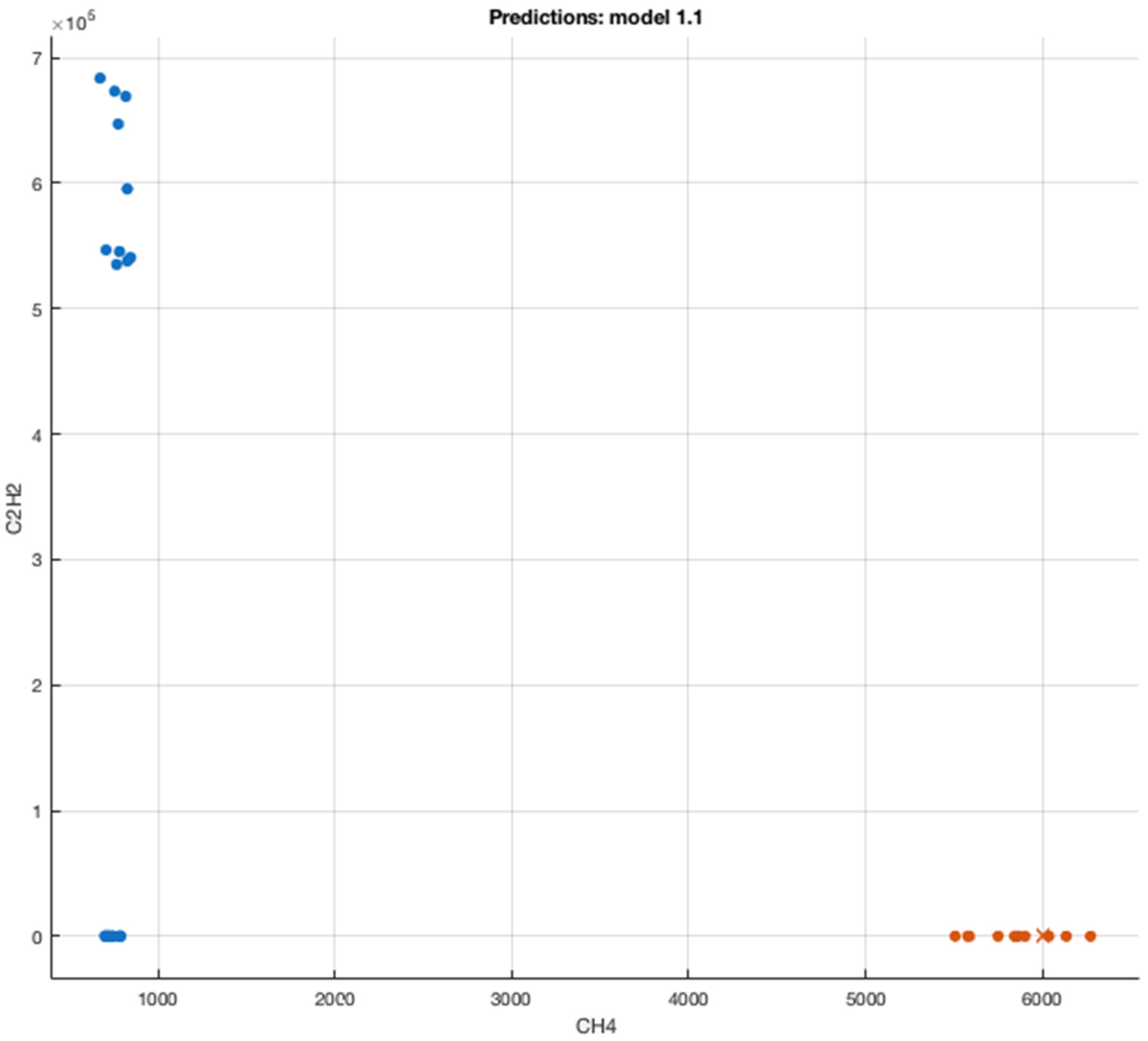
• Initially, the concentration levels of five feature gases are ingested as inputs to the first SVM (SVM 1). It will distinguish whether the oil samples represent a normal or faulty condition. If the sample is in normal condition, the algorithm ends.
• Secondly, if the SVM1 output has identified a fault condition, it is further ingested as input to the second SMV (SVM 2) which then distinguishes whether the fault is a thermal fault class or an electric discharge fault.
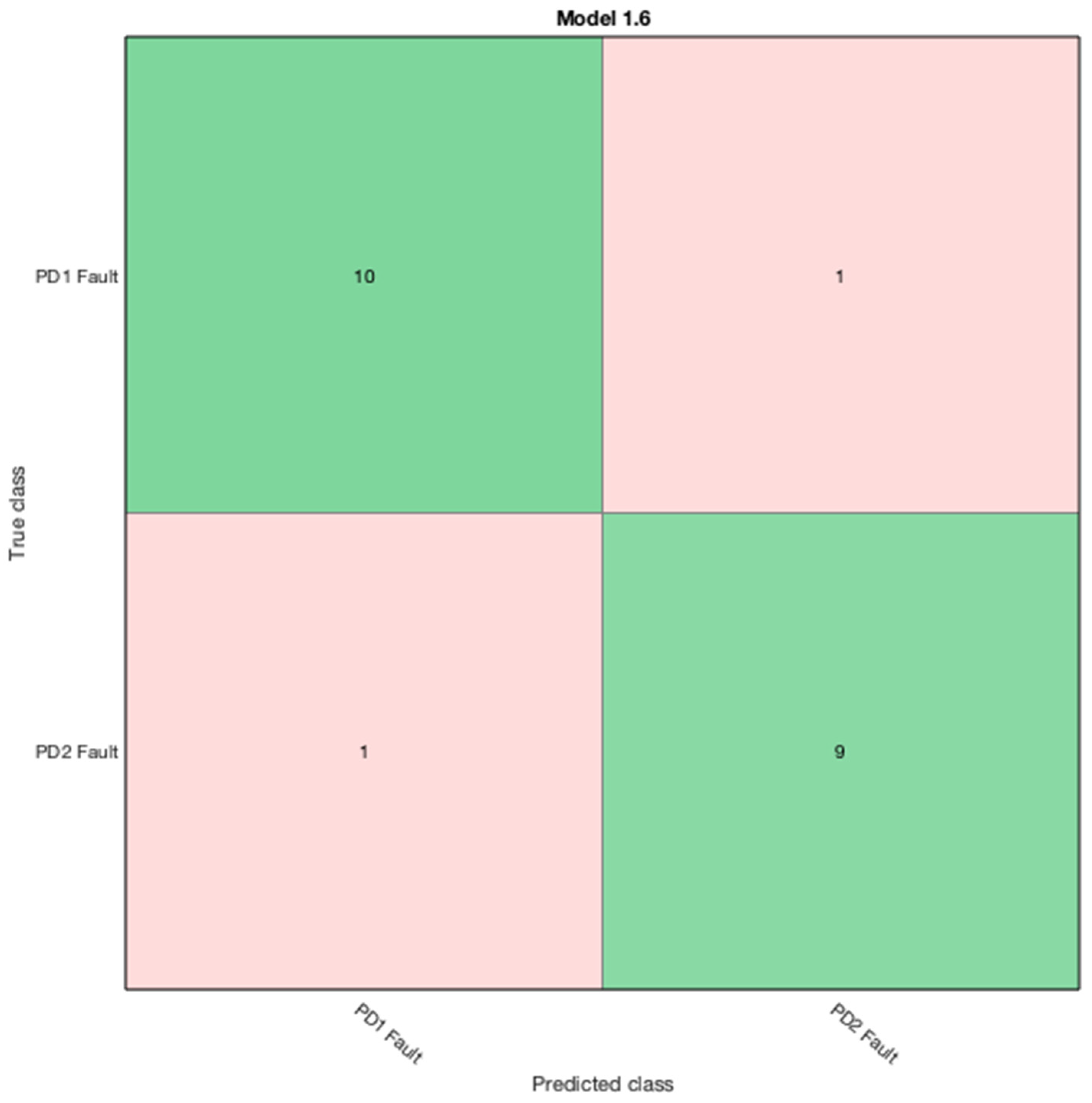
• Thirdly, if the fault class is pigeonholed as a PD fault, then it will be ingested as input to the third SVM (SVM 3), which will then distinguish whether the fault is PD1 or PD2.
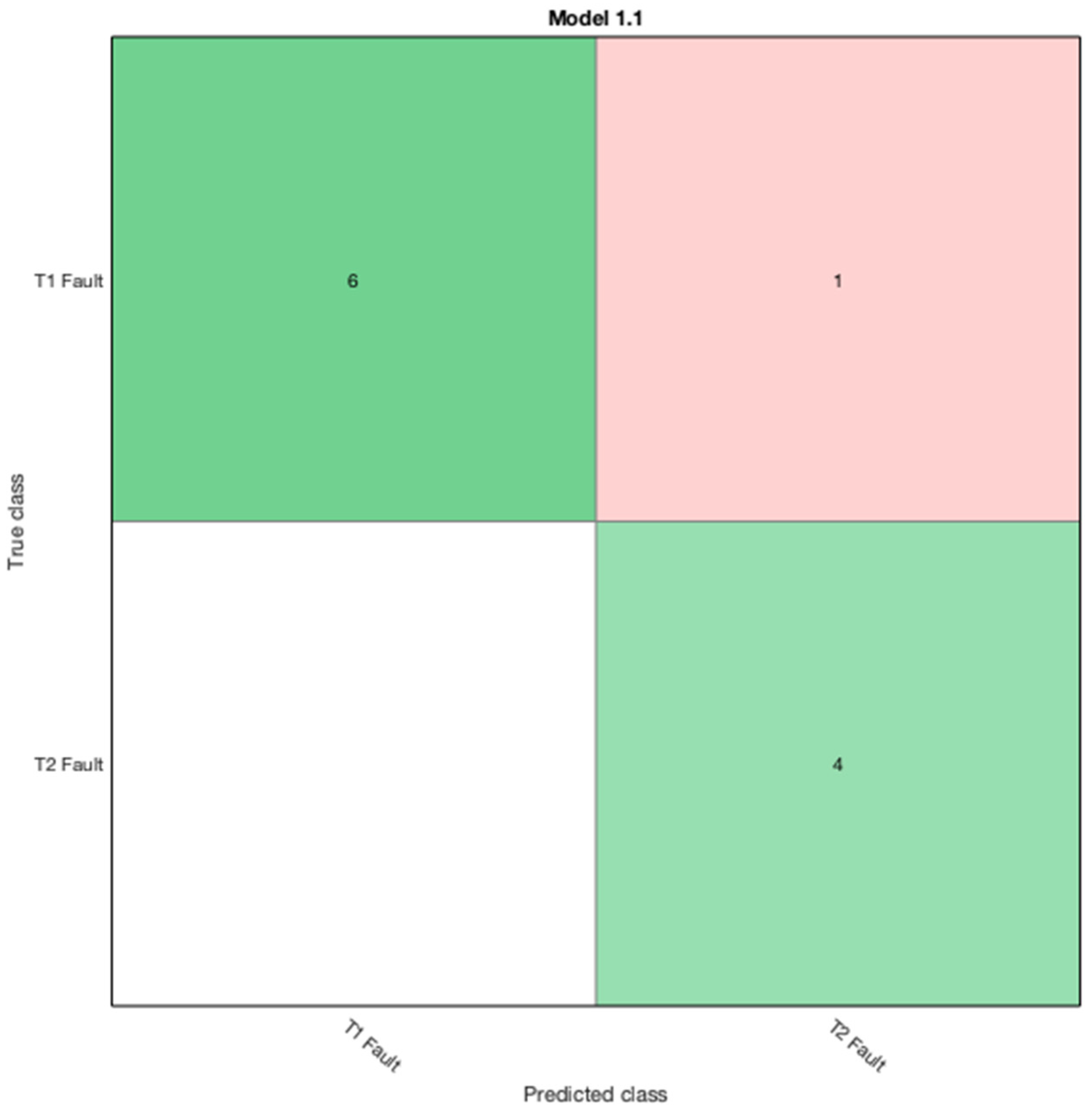
• At the same time, if the fault is categorized as a thermal (T) fault, then it will be ingested as input to the fourth SVM (SVM 4) which will distinguish whether the fault is a T1 or T2 fault as demonstrated.

To evaluate the statistical significance of the experimental DGA dataset, a single-factor ANOVA was employed. The results are illustrated in Table 2.

Table 2. Statistical analysis of experimental DGA dataset.

Source of Variation	SS	df	MS	F	p-Value	F Crit
Between Groups	4.7231 × 1011	5	9.4463 × 1010	5.33534763	9.1433 × 10−5	2.23578833
Within Groups	7.3299 × 1012	414	1.7705 × 1010
Total	7.8022 × 1012	419

It can be observed from the p-value of 9.1433 × 10⁻⁵ (<α = 0.05), that the experimental DGA results are statistically significant.

The sensitivity analysis of the input gases was carried out by adopting descriptive statistics analysis (DSSA), as shown in Table 3. DSSA examines the quantitative performance of the input dataset features.

Table 3. Descriptive statistics sensitivity analysis of input gases.

Parameter	H2	CH4	C2H2	C2H4	C2H6	CO
Mean	38,978.9143	28,260.8571	10,6671.346	94,012.2143	29,719.6571	24,078.9143
Standard Error	13,315.308	10,012.6008	25,868.0788	19,828.9585	10,192.548	8590.25301
Median	3895.5	835	311.5	4908	4028.5	3269
Mode	0	744	2	11	220	300
Standard Deviation	111,403.859	83,771.4282	21,6427.875	165,900.97	85,276.9749	71,871.2131
Sample Variance	1.2411 × 1010	7,017,652,184	4.6841 × 1010	2.7523 × 1010	7,272,162,445	5,165,471,270
Kurtosis	8.06695552	11.282565	1.63684628	0.37595746	9.53422061	11.585725
Skewness	3.0627171	3.35926699	1.8135374	1.47653406	3.22003396	3.52177109
Range	487,297	449,556	683,643	478,904	404,053	348,857
Minimum	0	0	0	0	0	0
Maximum	487,297	449,556	683,643	478,904	404,053	348,857
Sum	2,728,524	1,978,260	7,466,994.22	6,580,855	2,080,376	1,685,524
Count	70	70	70	70	70	70
Confidence Level (95.0%)	26,563.3126	19,974.592	51,605.4051	39,557.6899	20,333.5769	17,137.0858

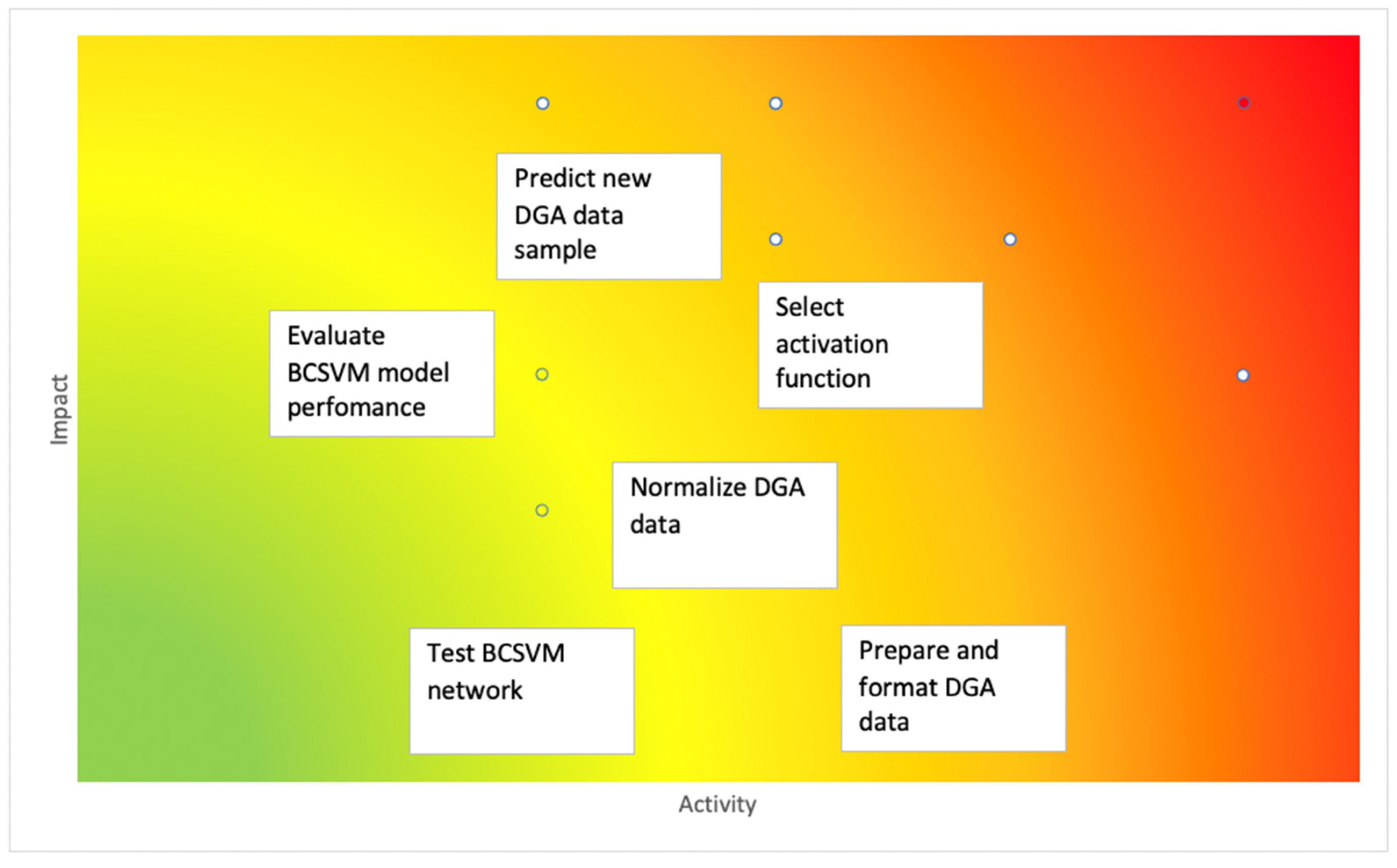
The complexity of the proposed solution design is demonstrated in Figure 4. The latter is partially based upon the related state of the problem diagnosing transformer faults and solution of DGA and artificial intelligence knowledge. Additionally, this can be illustrated in terms of a solution design complexity heatmap comprising all the main activities undertaken.

Figure 4. Complexity of the proposed BCSVM classification tree.

The red regions reveal locales of conceivably sheer complexity. The green regions denote locales of conceivably little complexity.

3. Results

In this section, the results are presented and discussed. The transformer oil testing samples based on mineral oil were abstracted from a South African transformer manufacturer after laboratory analysis. The BCSVM training phase was ingested with 70% of the oil testing samples and tested using 30% of the transformer oil samples. This investigation was conducted by employing the classification learner app in the MATLAB_R2018a software platform. Once the oil samples dataset was trained, the veracity of the distinctive SVMs was corroborated. The configuration matrix of a particular SVM that provides the highest degree of accuracy was selected and imported to predict the new testing data sample. The fault class prediction for the new data sample is carried out by utilizing Equation (7).

$$yfit=fitcecoc\left(Tbl, ResponseVarName\right)$$

(7)

Here,

$Tbl—$Multiclass predictor variables in table

$ResponseVarName—$Response variables

3.1. Training and Testing of SVM 1

The training and testing of SVM 1 are designed to categorize between the transformer’s normal and faulty conditions. The training stage was carried out using 70 oil samples with fault and normal conditions. A total of 14 oil data samples were then used in testing SVM 1. The results indicated that all the new oil data samples were pigeonholed accurately. The selection response and predictors selected by SVM1 using the ingested data are demonstrated in Figure 5. A 30-fold cross-validation has been selected.

Figure 5. The dataset variables were selected by the SVM 1 classifier.

The dissolved gases were automatically placed as the predictors and the fault type as the response. In the SVM 1 algorithm ${\mathrm{H}}_2$ and ${\mathrm{C}}_2{\mathrm{H}}_2$ was considered to acquire the desired output. The characterization of ${\mathrm{H}}_2$ versus ${\mathrm{C}}_2{\mathrm{H}}_2$ is illustrated in Figure 6.

Figure 6. ${\mathrm{H}}_2$ versus ${\mathrm{C}}_2{\mathrm{H}}_2$. Blue and orange (•)—raw data, orange and blue (×)—predicted data.

Further, various ML algorithms, i.e., linear SVM, quadratic SVM, cubic SVM, fine gaussian SVM, medium Gaussian SVM, and coarse Gaussian SVM, are compared in terms of accuracy (%), prediction speed (objects/sec) and training time (sec), as tabulated in Table 4. The testing and calculation of the accuracy of referenced algorithms tested on the same data were evaluated based on the percentage of accuracy to classify fault type, the prediction speed and the training time of the respective algorithm.

Table 4. SVM 1 DGA classification outcomes.

Type	Accuracy (%)	Prediction Speed	Training Time (sec)
Linear SVM	81.4	260	7.0125
Quadratic SVM	92.9	360	1.6171
Cubic SVM	58.6	370	53.793
Fine Gaussian SVM	80.0	360	1.3882
Medium Gaussian SVM	68.6	380	1.4147
Coarse Gaussian SVM	68.6	340	1.4259

In the SVM 1 algorithm$,$ the quadratic SVM provides the highest degree of accuracy, and the corresponding configuration matrix shown in Figure 7 was imported to the workspace to predict the new testing data samples.

Figure 7. SVM 1 confusion matrix.

3.2. Training and Testing of SVM 2

The training and testing of SVM 2 were purposed to categorize between PD and T faults. The training stage was carried out by using a total of 15 oil data samples with T fault and with PD fault conditions respectively. Subsequently, a total of 15 oil data samples were utilized in testing SVM2. The results indicated that a total of 14 oil data samples were classified accurately. The selection of the response and predictors selected by SVM 2 using this ingested data is demonstrated in Figure 8. A 30-fold cross-validation was selected.

Figure 8. The dataset variables selected by the SVM 2 classifier.

The dissolved gases were automatically placed as the predictors and the fault type as the response. In the SVM 2 algorithm, ${\mathrm{CH}}_4$ and ${\mathrm{C}}_2{\mathrm{H}}_2$ were considered to acquire the desired output. The characterization of ${\mathrm{CH}}_4$ versus ${\mathrm{C}}_2{\mathrm{H}}_2$ is illustrated in Figure 9.

Figure 9. ${\mathrm{CH}}_4$ versus ${\mathrm{C}}_2{\mathrm{H}}_2$. Blue and orange (•)—raw data, orange and blue (×)—predicted data.

Further, the various ML algorithms were compared in terms of accuracy (%), prediction speed (objects/sec) and training time (sec), as tabulated in Table 5.

Table 5. SVM 2 DGA classification outcomes.

Type	Accuracy (%)	Prediction Speed	Training Time (sec)
Linear SVM	96.9	170	2.0822
Quadratic SVM	81.2	180	1.3123
Cubic SVM	81.2	170	1.3312
Fine Gaussian SVM	96.9	170	1.3723
Medium Gaussian SVM	96.9	140	1.5766
Coarse Gaussian SVM	96.9	120	1.9193

In the SVM 2 algorithm$,$ the linear SVM, fine Gaussian SVM, medium Gaussian SVM and coarse Gaussian SVM provided the highest degree of accuracy and the coarse corresponding configuration matrix shown in Figure 10 was imported to the workspace to predict the new testing data samples.

Figure 10. Confusion matrix for SVM 2 classifier.

3.3. Training and Testing of SVM 3

SVM 3 was trained and tested to classify PD1 and PD2 faults. The training stage was conducted by using a total of 8 oil data samples with a PD1 fault condition and a total of 7 data samples with a PD2 fault condition. Therefore, a total of 10 data samples were utilized in the testing of SVM. The results indicated that all the data samples were pigeonholed accurately. The selection of responses and predictors selected by SVM 3 using the ingested data is demonstrated in Figure 11.

Figure 11. The dataset variables were selected by the SVM 3 classifier.

The dissolved gases were automatically placed as the predictors and the fault type as the response. In the SVM 3 algorithm, ${\mathrm{C}}_2{\mathrm{H}}_2$ and ${\mathrm{C}}_2{\mathrm{H}}_4$ were considered to acquire the desired output. The characterization of ${\mathrm{C}}_2{\mathrm{H}}_2$ versus ${\mathrm{C}}_2{\mathrm{H}}_4$ is illustrated in Figure 12.

Figure 12. ${\mathrm{C}}_2{\mathrm{H}}_2$ versus ${\mathrm{C}}_2{\mathrm{H}}_4$. Blue and orange (•)—raw data, orange and blue (×)—predicted data.

Further, the ML algorithms, were compared in terms of accuracy (%), prediction speed (objects/sec) and training time (sec), as tabulated in Table 6.

Table 6. SVM 3 DGA classification outcomes.

Type	Accuracy (%)	Prediction Speed	Training Time (sec)
Linear SVM	95.2	160	1.465
Quadratic SVM	95.2	160	0.967
Cubic SVM	100	130	1.008
Fine Gaussian SVM	90.5	150	0.989
Medium Gaussian SVM	90.5	160	0.941
Coarse Gaussian SVM	90.5	140	1.055

In the SVM 3 algorithm$,$ linear SVM, quadratic SVM, and cubic SVM provided the highest degree of accuracy, with cubic SVM yielding 100% accuracy, and the corresponding configuration matrix shown in Figure 13 was imported to the workspace to predict the new testing data samples.

Figure 13. Confusion matrix for SVM 3 classifier.

3.4. Training and Testing of SVM 4

The training and testing of SVM 4 were purposed to categorize between T1 and T2 fault classes. SVM 4 was trained by a total of 8 data samples with a T1 fault condition and a total of 7 data samples with a T2 fault condition. Consequently, a total of 10 data samples were used in testing SVM 4 and the results showed that 9 data samples were classified fittingly. The complete BCSVM was tested using 26 DGA data samples, and 24 samples were pigeonholed rightly. The precision of the overall BCSVM was 92%. The selection of responses and predictors selected by SVM 4 using the ingested data are demonstrated in Figure 14.

Figure 14. The dataset variables were selected by the SVM 4 classifier.

The dissolved gases were automatically placed as the predictors and the fault type as the response. In the SVM 3 algorithm, ${\mathrm{H}}_2$ and ${\mathrm{CH}}_4$ were considered to acquire the desired output. The characterization of ${\mathrm{H}}_2$ versus ${\mathrm{CH}}_4$ is illustrated in Figure 15.

Figure 15. ${\mathrm{H}}_2$ versus ${\mathrm{CH}}_4$. Blue and orange (•)—raw data, orange and blue (×)—predicted data.

Further, the ML algorithms were compared in terms of accuracy (%), prediction speed (objects/sec) and training time (sec), as tabulated in Table 7.

Table 7. SVM 4 DGA classification outcomes.

Type	Accuracy (%)	Prediction Speed	Training Time (sec)
Linear SVM	90.9	470	0.629
Quadratic SVM	100	480	0.253
Cubic SVM	90.9	390	0.242
Fine Gaussian SVM	100	410	0.254
Medium Gaussian SVM	100	390	0.275
Coarse Gaussian SVM	63.6	380	0.259

In the SVM 4 algorithm$,$ quadratic SVM, fine Gaussian SVM, and medium Gaussian SVM provided the highest degree of accuracy and the corresponding configuration matrix shown in Figure 16 was imported to the workspace to predict the new testing data samples.

Figure 16. Confusion matrix for SVM 4.

4. Case Studies

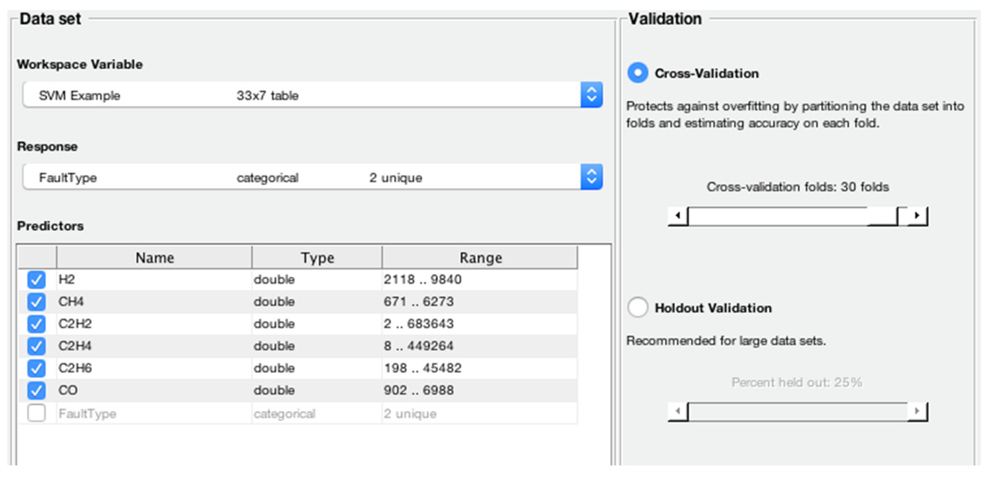
In this section, various transformer case studies are presented to corroborate the efficacy of the proposed BCSVM algorithm in identifying faults of an unknown dataset to the proposed algorithm learning process. The training and testing of the datasets were not examined from the same utility. The training data adopted from service field oil sample data and the testing oil sample dataset were established by physical unit inspection, as shown in Table 6. The latter will be an opportunity for examination of the proposed algorithm in a more indubitable approach and realizing the capability to development of an efficacious ML algorithm for field data enactment. In the proposed approach, six ML algorithms are assessed for examining the correlation between the response and predictors.

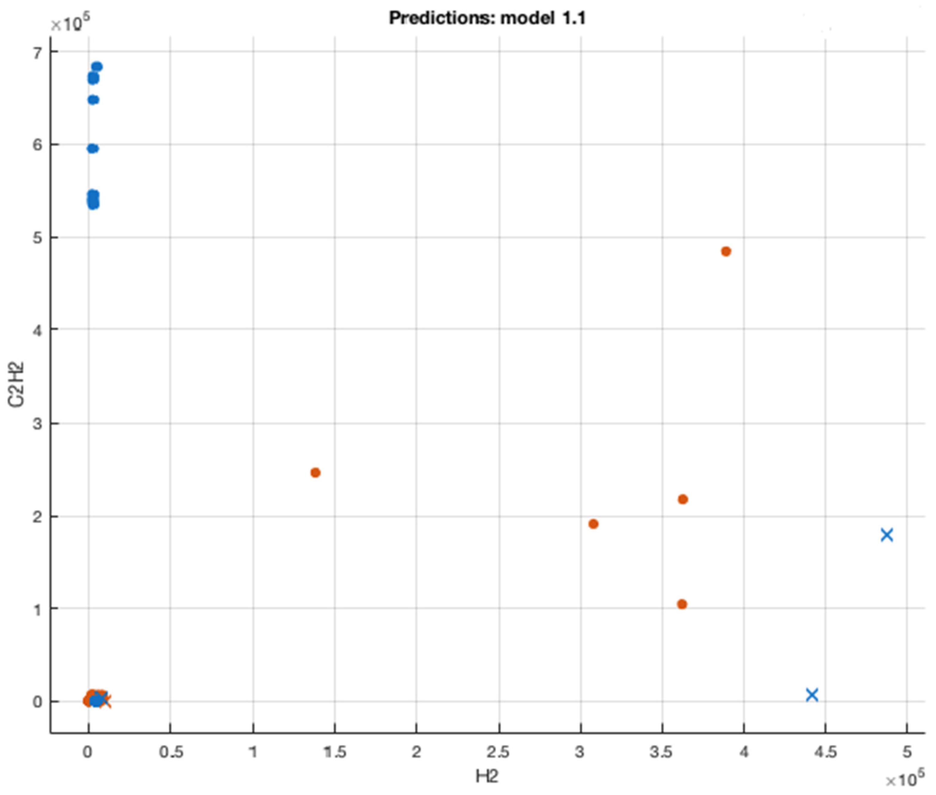
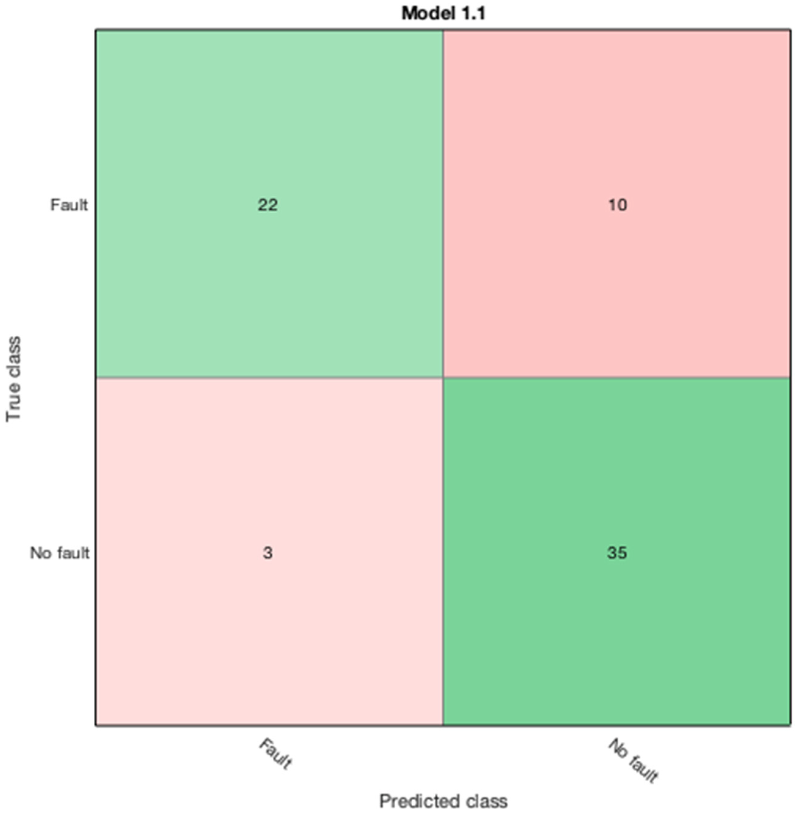
The proposed BCSVM is evaluated in Table 8 against the actual, ANN and IECGR techniques on a set of transformers’ DGA data that was not included in the training of the proposed algorithm. A major strength of BCSVM is the 30-fold cross-validation performance to circumvent overfitting problems.

Table 8. DGA fault classification case studies.

H2	CH4	C2H4	C2H6	C2H2	Actual	ANN	IECGR	BCSVM
302	490	360	182	95	T2	T2	ND *	T2
32	2	1	1	0.05	PD1	PD2	PD1	PD1
13	9	6	41	0	NF	NF	NF	NF
156	128	35	97	0	T1	T1	ND *	T1
596	81	90	10	245	PD2	PD2	PD2	PD2
23	41	7	37	2	T1	T2	T1	T1
1772	3631	8481	1071	79	T2	T2	T2	T2
87	31	36	11	30	PD2	PD2	PD2	PD2
35	40	41	10	10	PD2	PD2	PD2	PD2
143	4	9	3	2	PD2	PD2	PD2	PD2
2587.2	7.882	1.4	4.7004	0	PD1	PD1	PD1	PD1
1676	653	1006	81	418	PD2	PD2	PD2	PD2
181	262	528	210	0	T2	T2	T2	T2
181	176	51	76	5	T1	T2	T1	T1

* ND—not detectable.

From Table 6, it is observed that the fault class tag T2 has low accuracy against the actual data. Intriguingly, all other fault class tags performed well in the context of accuracy. Additionally, the IECGR was unable to conclusively diagnose some of the faults due to the limitations of the code ratios. Further, the proposed technique constitutes proof that it can be reliably applied in the prediction of unknown oil sample datasets, predicting all the case studies accurately.

5. Conclusions

The BCSVM construction for fault diagnosis of power transformers has been represented. Several faults are unpredictable by the IEC gas ratio (IECGR) method, which results in an undetectable conclusion. When using ANN, given that it is excellent at learning, the restraint of the inability of fuzzy logic to adapt the created rule base with the varying system for indivisible and irregular data is eradicated. Nonetheless, ANN has the hindrance of overfitting; therefore, it has lower generalization capability and provides circumscribed precision to fault identification. To circumvent all these challenges, in this work, power transformer fault identification was conducted by employing a binary classification support vector machine (BCSVM). The case study results demonstrate that the proposed BCSVM technique has a higher degree of diagnostic accuracy than the IECGR and ANN methods owing to its enhanced generalization capability, and it can classify indivisible DGA datasets by utilizing the kernel function.

References

1. Gouda, O.E.; El-Hoshy, S.H.; Ghoneim, S.S.M. Enhancing the Diagnostic Accuracy of DGA Techniques Based on IEC-TC10 and Related Databases. IEEE Access 2021, 9, 118031–118041. [Google Scholar] [CrossRef]
2. Draper, Z.H.; Dukarm, J.J.; Beauchemin, C. How to Improve IEEE C57.104-2019 DGA Fault Severity Interpretation. In Proceedings of the IEEE/PES Transmission and Distribution Conference and Exposition (T&D), New Orleans, LA, USA, 25–28 April 2022; pp. 1–5. [Google Scholar] [CrossRef]
3. Ward, S.A.; El-Faraskoury, A.; Badawi, M.; Ibrahim, S.A.; Mahmoud, K.; Lehtonen, M.; Darwish, M.M.F. Towards Precise Interpretation of Oil Transformers via Novel Combined Techniques Based on DGA and Partial Discharge Sensors. Sensors 2021, 21, 2223. [Google Scholar] [CrossRef] [PubMed]
4. Emara, M.M.; Peppas, G.D.; Gonos, I.F. Two Graphical Shapes Based on DGA for Power Transformer Fault Types Discrimination. IEEE Trans. Dielectr. Electr. Insul. 2021, 28, 981–987. [Google Scholar] [CrossRef]
5. Kherif, O.; Benmahamed, Y.; Teguar, M.; Boubakeur, A.; Ghoneim, S.S.M. Accuracy Improvement of Power Transformer Faults Diagnostic Using KNN Classifier with Decision Tree Principle. IEEE Access 2021, 9, 81693–81701. [Google Scholar] [CrossRef]
6. Zhang, Y.; Chen, H.C.; Du, Y.; Chen, M.; Liang, J.; Li, J.; Fan, X.; Sun, L.; Cheng, Q.S.; Yao, X. Early Warning of Incipient Faults for Power Transformer Based on DGA Using a Two-Stage Feature Extraction Technique. IEEE Trans. Power Deliv. 2022, 37, 2040–2049. [Google Scholar] [CrossRef]
7. Haque, N.; Jamshed, A.; Chatterjee, K.; Chatterjee, S. Accurate Sensing of Power Transformer Faults from Dissolved Gas Data Using Random Forest Classifier Aided by Data Clustering Method. IEEE Sens. J. 2022, 22, 5902–5910. [Google Scholar] [CrossRef]
8. Taha, I.B.M.; Ibrahim, S.; Mansour, D.E.A. Power Transformer Fault Diagnosis Based on DGA Using a Convolutional Neural Network with Noise in Measurements. IEEE Access 2021, 9, 111162–111170. [Google Scholar] [CrossRef]
9. Kaur, K.; Sharma, N.K.; Singh, J.; Bhalla, D. Performance Assessment of IEEE/IEC Method and Duval Triangle technique for Transformer Incipient Fault Diagnosis. In 2022 IOP Conference Series: Materials Science and Engineering; IOP Publishing: Bristol, UK, 2022; Volume 1228, p. 012027. [Google Scholar] [CrossRef]
10. Ekojono, R.A.P.; Apriyani, M.E.; Rahmanto, A.N. Investigation on machine learning algorithms to support transformer dissolved gas analysis fault identification. Electr. Eng. 2022, 104, 3037–3047. [Google Scholar] [CrossRef]
11. Saravanan, D.; Hasan, A.; Singh, A.; Mansoor, H.; Shaw, R.N. Fault Prediction of Transformer Using Machine Learning and DGA. In Proceedings of the 2020 IEEE International Conference on Computing, Power and Communication Technologies (GUCON), Greater Noida, India, 2–4 October 2020; pp. 1–5. [Google Scholar] [CrossRef]
12. Benmahamed, Y.; Kherif, O.; Teguar, M.; Boubakeur, A.; Ghoneim, S.S.M. Accuracy Improvement of Transformer Faults Diagnostic Based on DGA Data Using SVM-BA Classifier. Energies 2021, 14, 2970. [Google Scholar] [CrossRef]
13. Wu, Y.; Sun, X.; Zhang, Y.; Zhong, X.; Cheng, L. A Power Transformer Fault Diagnosis Method-Based Hybrid Improved Seagull Optimization Algorithm and Support Vector Machine. IEEE Access 2022, 10, 17268–17286. [Google Scholar] [CrossRef]
14. Zeng, B.; Guo, J.; Zhu, W.; Xiao, Z.; Yuan, F.; Huang, S. A Transformer Fault Diagnosis Model Based on Hybrid Grey Wolf Optimizer and LS-SVM. Energies 2019, 12, 4170. [Google Scholar] [CrossRef]
15. Ma, H.; Zhang, W.; Wu, R.; Yang, C. A Power Transformers Fault Diagnosis Model Based on Three DGA Ratios and PSO Optimization SVM. In Proceedings of the Conference on Mechatronics and Electrical Systems (ICMES 2017), Wuhan, China, 15–17 December 2017; p. 339. [Google Scholar] [CrossRef]
16. Yu, W.; Yu, R.; Li, C. An Information Granulated Based SVM Approach for Anomaly Detection of Main Transformers in Nuclear Power Plants. Sci. Technol. Nucl. Install. 2022, 2022, 3931374. [Google Scholar] [CrossRef]
17. El-kenawy, E.S.M.; Albalawi, F.; Ward, S.A.; Ghoneim, S.S.M.; Eid, M.M.; Abdelhamid, A.A.; Bailek, N.; Ibrahim, A. Feature Selection and Classification of Transformer Faults Based on Novel Meta-Heuristic Algorithm. Mathematics 2022, 10, 3144. [Google Scholar] [CrossRef]
Publisher’s Note: MDPI stays neutral with regard to jurisdictional claims in published maps and institutional affiliations.
Article Metrics
Citations
Article Access Statistics
Multiple requests from the same IP address are counted as one view.