Article

Distributionally Robust Optimization of an Integrated Energy System Cluster Considering the Oxygen Supply Demand and Multi-Energy Sharing

1
College of Water Conservancy and Civil Engineering, Tibet Agriculture and Animal Husbandry University, Linzhi 860000, China
2
School of Electrical Engineering, Tibet Agriculture and Animal Husbandry University, Linzhi 860000, China
*
Author to whom correspondence should be addressed.
Energies 2022, 15(22), 8723; https://doi.org/10.3390/en15228723
Submission received: 20 October 2022 / Revised: 15 November 2022 / Accepted: 17 November 2022 / Published: 20 November 2022
(This article belongs to the Topic Integration of Renewable Energy)

Abstract

:
Regional integrated energy systems (IESs) have emerged to satisfy the increasing diversified energy demand in Tibet. However, limited resource allocation of a given IES can occur because of the uncertainty in the output and prediction error of distributed renewable energy (DRE). A distributionally robust optimization (DRO) model was proposed for the joint operation of multiple regional IESs, and multi-energy sharing and multi-energy flow coupling of electricity, heat, and oxygen were considered. The probability distribution of the DRE output was described using 1 norm and norm constraints, and the minimum operating cost under adverse scenarios was determined through DRO. Furthermore, on the premise of ensuring cluster profit, a pricing mechanism of the energy supply within the cluster was proposed. Finally, a typical model involving eight cases was established and analyzed. The results revealed that multi-energy sharing and multi-energy flow coupling improved the economy of IES cluster operation and realized the coordination of robustness and economy. The energy supply price within the cluster enhanced enthusiasm on the demand side.

1. Introduction

Altitude stress due to hypoxia has greatly affected the health and quality of life of residents in plateau areas. The government and researchers have explored how to solve the plateau oxygen supply problem. Tibet has proposed a universal oxygen supply in plateau urban areas as a development goal [1,2,3]; China has promoted and is working toward emission peak and carbon neutrality targets. As a clean energy base, Tibet has proposed a series of energy development plans. However, it is limited by inefficient energy utilization and increasing penetration of distributed renewable energy (DRE); the increasing electric and oxygen demand and low absorption rate of DRE pose new challenges to energy system construction in Tibet.
As a new energy system to promote sustainable energy development, an integrated energy system (IES) could effectively improve energy utilization efficiency while meeting diversified energy demands within the system. Compared with the existing energy framework in Tibet, the combination of source-network-load-storage modular interactions and integrated interactions in IESs has significantly altered the construction of energy systems and improved power grid resilience, and these benefits can be harnessed to meet the unique demand for a dispersed oxygen supply on the plateau. However, multi-energy flow coupling and the existence of multiple time scales result in IES operation difficulties. Current research mainly focuses on the optimal strategy of a single IES. In [4], system investment and operation costs were reduced by considering source storage capacity allocation and operation optimization. In [5,6,7], power-to-gas (P2G) technology was used to realize the consumption of renewable energy and improve the economic benefits of the system. In [8,9], a dynamic energy hub and planning model was built, and an optimal planning and operation scheme of the IES was achieved. However, there is little research on the optimal scheduling problem of IES clusters. The existing research on P2G mainly focuses on the hydrogen energy of power-to-hydrogen (P2H) units and methanated natural gas utilization, but there is no research on P2H oxygen utilization in the P2G process.
Relevant research on plateau oxygen supply has shown that the feasibility and economic benefits of the vacuum pressure swing adsorption (VPSA) method in plateau areas are greater than those of the cryogenic air and membrane separation methods [10,11,12]. However, the disparities between oxygen supply demand, electric demand, and electric supply are becoming more pronounced as Tibet’s economy continues to develop. The efficient use of energy cannot be facilitated by VPSA oxygen supply alone. Therefore, this study investigates a more effective oxygen supply mode that reduces VPSA’s electricity requirements.
The resource allocation capacity of a single IES is limited. The limitations of the energy framework create problems such as uncertainty in the DRE output, prediction error [13], and low consumption rates. Scholars have proposed combining multiple regional IESs, forming an alliance mechanism through multiple regional IESs, and building an IES cluster scheduling system. Energy sharing interactions among IESs could be realized to improve energy utilization efficiency and energy supply levels, achieve the best overall benefits, and reduce the impact of the energy framework on system scheduling. However, existing methods for the operation of multiple IESs do not accurately capture system operation characteristics in real time or highlight energy sharing among clusters [14]. Therefore, an IES cluster needs to account for the collaborative multi-energy interactions between multiple IESs, butthe current study focuses on electricity sharing [15].
DRE output uncertainty significantly affects power system safety and economy. Currently, the main methods targeting uncertainty in power systems are stochastic optimization (SO) [16,17,18] and robust optimization (RO) [19,20,21]. However, SO and RO have shortcomings. Scholars have used distributionally robust optimization (DRO) to address uncertainty [22,23,24]. DRO is based on historical data and can be employed to determine the uncertainty set containing possible distributions and obtain the optimal solution when the prediction error of uncertainty factors follows the worst probability distribution. Through correlation transformation, the DRO can be converted into a deterministic mixed integer linear programming (MILP) model. This model can be directly solved by using Groubi. Many studies have examined DRO applications in the IES [25,26,27,28], but DRO has not been applied in IES cluster optimization. Due to the difficulty of controlling electricity, heat, and oxygen coupling and the coordination and synergy among multiple clusters, IES clusters are highly uncertain. It is difficult to address IES cluster uncertainty using conventional RO and SO techniques. Therefore, research on IES cluster operation based on DRO is critical.
In this study, a DRO strategy for IES clusters was proposed, which considered the oxygen supply demand in plateau areas and multiple energy sharing. Under both 1 norm and norm constraints, a scheduling strategy for coordinating system robustness and model economy was constructed through multiple energy sharing mechanisms. The main contributions of this paper are as follows:
(1)
Based on the energy demand, energy framework and energy development planning in Tibet, a multi-energy flow coupling IES architecture of electricity, heat, oxygen, and other energy sources was established by coupling concentrated solar power (CSP), P2H, and other equipment.
(2)
The scenario uncertainty was described by combining the uncertainty probability distribution confidence set constrained by both the 1 norm and norm, and the worst scenario probability distribution was determined.
(3)
To minimize the IES cluster operation cost, a cooperative optimization strategy considering IES cluster robustness and economy was established through double-norm constraints and multiple energy sharing mechanisms. Furthermore, the comprehensive model effect was verified by comparing several cases.
The remainder of this paper is organized as follows: Section 2 introduces the IES cluster, Section 3 describes the structure and operation strategy of the two-stage DRO model, Section 4 presents the optimization framework, data, and model simulation results, and Section 5 summarizes the main findings, relevant limitations, and further research directions.

2. IES Cluster

2.1. IES Architecture

The IES architecture is shown in Figure 1. Dispatching of a single IES typically involves controllable units (CSP, hydropower (HP), P2H, hydrogen fuel cells (HFC), VPSA, demand response load, an electric furnace (EF), and other units), uncontrollable units (distributed wind/photovoltaic energy units, hydrogen charging stations, etc.), and energy storage equipment (hydrogen gas storage (HGS), etc.). To satisfy the energy demand and emission peak and carbon neutrality targets, a dispatching center was set up in the proposed regional IES to couple the various equipment and energy sources and convert the various renewable energy sources, such as external electric energy and hydrogen energy, into the required energy sources.
P2H and methanation reactors were included as traditional power-to-gas technology options, and the low efficiency of methanation reactors and carbon emissions associated with natural gas consumption were considered. Following the energy development plan of Tibet, this paper proposed the utilization of oxygen and hydrogen in P2H products according to local conditions. The heat supply was replaced by HFC, EF, and CSP units. Oxygen was supplied by collecting P2H oxygen combined with VPSA technology. Hydrogen was used by hydrogen charging stations, which could provide hydrogen energy for hydrogen internal combustion electric vehicles (HICEVs), and HICEVs were included among the buses, taxis, and official vehicles used in urban areas. This plan would not only reduce carbon emissions, but also improve energy utilization efficiency and promote the consumption of the output of distributed wind/photovoltaic energy systems.
A dispatching center was used to coordinate and control the IES aggregation unit. Following the real-time situation of electric and hydrogen energy demands, this approach can implement energy sharing interactions among clusters, and excess electric energy or hydrogen can be sold to the grid power (GP) or hydrogen networks (HN), respectively. Figure 1 shows that the load of the IES cluster can be categorized into uncontrollable and demand response loads. Among these loads, an uncontrollable load is the load whose use considerably influences the demand side and cannot be controlled, for example, electric lights or computers. The demand response load can be categorized into transferable and adjustable loads. The adjustable load includes equipment that functions intermittently, e.g., water boilers and humidifiers. The transferable load refers to the load of other household equipment that can be transferred to other periods of work, for example, centralized laundry units and dishwashers. Considering that the transfer of electrical and heat loads slightly impacts the oxygen supply demand, only the adjustable amount was considered for the oxygen load.

2.2. Multi-Energy Sharing Architecture

The multi-energy sharing architecture of the IES cluster is shown in Figure 2. The sharing of electricity, oxygen, and hydrogen was included. However, due to the high heat pipe loss, heat interaction among IES clusters was not considered. The IES multi-energy interaction flow is based on traditional electric energy interactions. Energy sources such as oxygen and hydrogen are shared at very low transmission loss and can not only replace the role of energy storage to a certain extent, but also ensure deeper energy sharing among IES clusters, thus effectively improving the overall cluster scheduling flexibility.
To satisfy the demand for multiple types of energy loads, optimization of the dispatch of IES clusters is critical. However, uncontrollable units occur in the cluster, namely DRE, whose output uncertainty could adversely affect cluster scheduling.

2.3. Probability Scenario

In this study, 10 scenario and probability values were generated for each IES, based on 180 days of data through Copula joint scenario generation and the k-means clustering algorithm as the initial probability scenario generation method. The 1 norm and norm were simultaneously included to constrain the confidence set of the uncertainty probability distribution. The column and constraint generation (CCG) algorithm was used to design a DRO strategy for multiple cases, considering these double-norm constraints. The relevant target values in the various cases were obtained via DRO, and the scenario probability values were modified according to the above double-norm constraints.

3. Distributionally Robust Optimization Model

The uncertainty in the DRE output and forecast error can adversely affect IES cluster planning and scheduling. Therefore, based on the above double-norm constraints, considering the energy demand in Tibet and the emission peak and carbon neutrality targets, a new IES cluster planning and scheduling strategy was constructed.

3.1. Objective Function

The model was optimized considering the IES cluster. When the cluster economy and robustness are coordinated through DRO, the objective function is as follows:
min { f b r + max i = 1 K ( p i T + 1 min f r i ) }
where p i T denotes the scenario probability value, f b r denotes the comprehensive equipment cost, and f r i denotes the total operation cost.
Following Equation (1), the objective function is the min−max−min form of DRO. In contrast to RO (RO can only optimize worst-scenario problems), DRO can solve worst-scenario one-stage planning schemes through the lower bound, estimate the economy of operation through min f r i , determine the worst operation scenario that the cluster may encounter through min f r i , and update the scenario probability value. The robustness and economy can be coordinated through continuous iteration.
The comprehensive cost f b r and operation cost f r i of the equipment are included in Equations (2) and (3), which can be calculated as follows:
{ f b r = f b ( 5 365 ( 1 + r ) ) f r i = f e i + f h i + f D R i + f D R E i + f E S i
f b = i = 1 K ( P r i . C S P M C S P i + P r i . P 2 H M P 2 H i + P r i . h s M h s i + P r i . V P S A M V P S A i + P r i . p i p L p i p i + P r i . H P M H P i + P r i . D R E M D R E i + P r i . E F M E F i + P r i . H F C M H F C i + C H R S i )
where P r i . C S P denotes the unit comprehensive cost of CSP units (RMB/kW), P r i . P 2 H denotes the unit comprehensive cost of P2H units (RMB/kW), P r i . h s denotes the unit comprehensive cost of HGS units (RMB/m3), P r i . V P S A denotes the unit comprehensive cost of VPSA technology (RMB/kW), P r i . p i p denotes the unit comprehensive cost of transmission pipelines (RMB/km), P r i . H P denotes the unit comprehensive cost of HP (RMB/kW), P r i . D R E denotes the unit comprehensive cost of DRE (RMB/kW), P r i . E F denotes the unit comprehensive cost of EFs (RMB/kW), P r i . H F C denotes the unit comprehensive cost of HFCs (RMB/kW), M P 2 H i denotes the P2H installed capacity, M h s i denotes the HGS installed capacity, M C S P i denotes the CSP installed capacity, M V P S A i denotes the VPSA installed capacity, M H P i denotes the HP installed capacity, M D R E i denotes the DRE installed capacity, M E F i denotes the EF installed capacity, M H F C i denotes the HFC installed capacity, L p i p i denotes the construction length of hydrogen and oxygen transmission pipelines, and C HRS i denotes the cost of transforming gas stations into hydrogen charging stations, where f e i denotes the electricity purchase and sale cost from the GP, f h i denotes the hydrogen gas purchase and sale cost from the HN, f D R i denotes the cost of the demand response, f E S i denotes the cost of using energy storage, and f D R E i denotes the cost of discarding solar and wind energy.
(1)
The electricity purchase and sale cost can be calculated as follows:
f e = t = 1 24 ( P r i b u y t P b u y . e t P r i s e l l t P s e l l . e t )
where P r i b u y t denotes the electric purchase price, P b u y . e t denotes the electric purchase amount, P s e l l . e t denotes the electric sale amount, and P r i s e l l t denotes the electric sale price.
(2)
The hydrogen gas purchase and sale cost can be calculated as follows:
f h = t = 1 24 ( P r i . h t P h . b u y t δ h P r i . h t P h . s e l l t )
where P r i . h t denotes the hydrogen purchase price, P h . b u y t denotes the hydrogen purchase amount, P h . s e l l t denotes the hydrogen sale amount, and δ h denotes the conversion coefficient of the purchase price.
(3)
The demand response cost can be calculated as follows:
f D R = δ t r t = 1 24 ( P t r t + H t r t ) + δ c u t t = 1 24 ( P c u t t + H c u t t + O c u t t )
where δ t r denotes the demand-side translation cost conversion coefficient and δ c u t denotes the demand-side adjustment cost conversion coefficient.
(4)
The cost of using energy storage can be calculated as follows:
f D R E = δ D R E t = 1 24 ( P P . D R E t P D R E t )
where δ D R E denotes the conversion coefficient of discarding solar and wind energy, P P . D R E t denotes the DRE supply, and P D R E t denotes the DRE consumption electric power.
(5)
The solar and wind costs can be calculated as follows:
f E S = δ H S t = 1 24 ( P H S . c h t + P H S . d i s t ) + δ h s t = 1 24 ρ h ( V h s . c h t + V h s . d i s t )
where P H S . c h t denotes the charging heat power, P H S . d i s t denotes the discharging heat power, V h s . c h t denotes the charging hydrogen volume, V h s . d i s t denotes the discharging hydrogen volume, δ H S denotes the heat storage (HS) cost per unit power, and δ h s denotes the hydrogen storage cost per unit volume.

3.2. P2H-VPSA Combined Oxygen Supply Model

The overall product utilization efficiency of P2G is low, and the utilization of oxygen in the P2H process has not been previously considered. Therefore, P2H was combined with HFC, HS, and VPSA units. The hydrogen generated by P2H could be used by HFCs, HS units, and hydrogen charging stations, and the generated oxygen could be used combined with the VPSA, oxygen storage, and oxygen supply loads to achieve efficient product utilization and partially meet oxygen supply requirements.
(1)
The P2H model can be expressed as follows:
{ P E L . h t = η P 2 H P E L t V E L . h t = P E L . h t / P H . e / ρ h V E L . O t = η P 2 H P E L t / P O . e / ρ O 0 P E L t M P 2 H Δ P E L l p P E L t P E L t 1 Δ P E L u p
where P E L . h t and P E L t denote the hydrogen production power and electric power consumption, respectively, at the P2H stage (kW); V E L . h t denotes the volume of hydrogen produced via P2H (m3/h); η P 2 H denotes the P2H energy conversion efficiency; ρ O denotes the oxygen density; P H . e denotes the power consumption for hydrogen production per unit mass (kW/kg); V E L . O t denotes the P2H oxygen production volume; P O . e denotes the power consumption for oxygen production per unit mass; M P 2 H denotes the P2H installed capacity; P E L min denote the electric power limit of P2H; and Δ P E L u p and Δ P E L l p denote the P2H limits of climbing power.
The thermoelectric ratio of HFCs can be adjusted to increase flexibility. The HFC model can be expressed as follows:
{ P H F C . e t = η H F C P H F C . h t V H F C . h t = η H . e P H F C . h t / P H . e / ρ H P H F C . h min P H F C . h t P H F C . h max 0 P H F C . h t M H F C η e . H min P H F C . e t P H F C . H t η e . H max P H F C . e t Δ P H F C . H l p P H F C . H t P H F C . H t 1 Δ P H F C . H u p
where P H F C . h t denotes the hydrogen consumption power of HFCs (kW), η H F C denotes the energy conversion efficiency of HFCs, P H F C . e t denotes the HFC electric power (kW), P H F C . H t denotes the HFC heat power (kW), V H F C . h t denotes the hydrogen consumption volume of HFCs (m3/h), η e . H max and η e . H min denote the heat power limit coefficients, Δ P H F C . H u p and Δ P H F C . H l p denote the HFC limits of climbing power, and M H F C denotes the HFC installed capacity.
(2)
The VPSA model can be expressed as follows:
{ V V P S A t = η V P S A P V P S A t / P V P S A . e P V P S A min P V P S A t M V P S A Δ P V P S A l p P V P S A t P V P S A t 1 Δ P V P S A u p
where P V P S A t denotes the VPSA power (kW), η V P S A denotes the highest economic efficiency of oxygen production, P V P S A . e denotes the unit power consumption (kW/m3), V V P S A t denotes the oxygen generation volume (m3/h), P V P S A max and P V P S A min denote the VPSA power limits, and Δ P V P S A u p and Δ P V P S A l p denote the VPSA limits of climbing power.

3.3. Oxygen Load Model

The oxygen load is based on the unit volume of oxygen delivery required to correct the altitude from 3000 to 1000 m, and the electrical and heat loads can be considered to correct the building volume at the oxygen supply site. This ensures that the oxygen load can meet the oxygen supply requirements with a flexible response; please refer to [12].
(1)
To simplify the calculation, the oxygen supply mode was divided into two cases based on the electrical and heat loads. When the electrical or heat load increases, it can be considered that there exists a new oxygen supply demand, the increment in the electrical or thermal load can be set to the oxygen delivery mode, and the invariant can be set to the maintenance mode. When the electrical or heat load decreases, it can be considered that there is no new oxygen supply demand, and the oxygen maintenance mode can be set. The oxygen delivery amount in the maintenance mode is the escape amount of oxygen. The oxygen load can be calculated as follows:
{ V O 2 = w ( Δ e ) / η e . a h C O 2 + ( 1 w ) ( Δ h ) / η h . a h C O 2 Δ e = P ( P L t P L t 1 ) Δ h = P ( H L t H L t 1 )
O L t = w ( P L t P L B t ) / η e . a h C O 2 η e s c + ( 1 w ) ( H L t H L B t ) / η h . a h C O 2 η e s c + V O 2
where V O 2 denotes the oxygen volume in the supply mode (m3/h); P ( ) denotes the preserved positive numbers in the matrix; P L t denotes the electrical load; P L B t denotes the electrical load without the oxygen supply demand; H L t denotes the heat load; H L B t denotes the heat load without the oxygen supply demand; w denotes the weight, which is 0.5 in winter and 1 in the other seasons; η e . a denotes the electricity consumption per unit area (W/m2); η h . a denotes the heat consumption per unit area (W/m2) (Table 1); C O 2 denotes the amount of oxygen delivered per unit area; .. denotes the height of a single-story building, which is 3 m; and η e s c denotes the oxygen escape amount, which is 50%. Table 1 provides the conversion coefficient between the power or heat supply and unit area.
(2)
The amount of oxygen delivered per unit area can be obtained as follows:
{ C O 2 = m 0 ρ O t m 0 = m 1 m
where m 0 denotes the oxygen content to be delivered (m3/h), t denotes the time, m 1 denotes the corrected oxygen mass content, and m denotes the oxygen mass content before correction.
{ m = ρ O λ η O λ = P / P 0 ln P = a ( H 10000 ) 3 + b ( H 10000 ) 2 + c ( H 10000 ) + d
where η O denotes the average proportion of oxygen in the atmosphere; P 0 denotes the atmospheric pressure at sea level; P denotes the atmospheric pressure at the current altitude; a , b , c , and d denote altitude correction factors (please refer to literature [29] for specific data); and H denotes the altitude.
{ m 1 = ρ O λ 1 η O λ 1 = P 1 / P 0
where H 1 denotes the correct altitude of the target. Please refer to the literature 12 for specific data. Moreover, P 1 denotes the correct atmospheric pressure of the target. Equation (15) can be employed to calculate ln P .

3.4. CSP Assembly Unit and Energy Balance Constraints

Please refer to Equations (A1)–(A10) in Appendix A for the other equipment constraints.
(1)
The heat fluid transmission loss at a CSP power plant is very low, so it was ignored. The CSP power plant constraints can be expressed as follows:
{ P S F , H T F t + P H S . d i s t = P H S . c h t + P C S P . H . e t P S F , H T F t = η S F , H T F S L P D t ρ P . L P P C S P . e t = η C S P P C S P . H . e t P C S P . H . e min P C S P . H . e t M C S P P C S P . H . e l p P C S P . H . e t P C S P . H . e t 1 P C S P . H . e u p
where P S F , H T F t denotes the heat power of the heat collector to transfer the heated fluid; P C S P . H . e t denotes the CSP steam turbine heat power supply; η S F , H T F denotes the photothermal efficiency of the heat collector; S L P denotes the heat receiver area, at 4 × 1 m2; D t denotes the solar intensity; ρ P . L P denotes the actual energy flow density irradiated to the heat receiver after superposition of the mirror surface; η C S P denotes the steam turbine efficiency; P C S P . e t denotes the CSP electric power; and P C S P . H . e l p and P C S P . H . e u p denote the CSP limits of climbing power.
(2)
The CSP-HS constraints can be expressed as follows:
{ S H t = S H t 1 + η S H c h P H S . c h t ( P C S P . H t + P H S . d i s t ) / η S H d i s S H min S H t S H max P H . c h min P H S . c h t α H . c h P H . c h max P H . d i s min P H S . d i s t α H . d i s P H . d i s max α H . d i s + α H . c h 1 S H t = 1 = S H t = 24 ( 2 t 24 )
where S H t denotes the HS capacity, S H max and S H min denote the limits of the HS capacity, α H . d i s denotes the discharging heat power status parameters, α H . c h denotes the charging heat power status parameters, P H . c h m a x and P H . c h min denote the limits of the charging heat power, P H . d i s max and P H . d i s min denote the limits of the discharging heat power, η S H c h denotes the charging heat power efficiency, η S H d i s denotes the discharging heat power efficiency, and P C S P . H t denotes the heat power supplied to the heat load.
(3)
The energy balance constraints can be expressed as follows:
P C S P . e t + P H P t + P D E R t + P H F C . e t + P b u y . e t = P s e l l . e t + P i a . e t + P E L . D R t + P E F . e t + P V P S A t + P E L t P C S P . H t + P E F . H t + P H F C . H t = P H L . D R t V V P S A t + V E L . O t = V O L . D R t + P i a . O t V E L . h t + V h s . d i s t + P h . b u y t = V H F C . h t + V h s . c h t + P h . s e l l t + P i a . h t s . t { 0 P b u y . e t P b u y . e max 0 P s e l l . e t P s e l l . e max 0 P h . s e l l t P h . s e l l max 0 P h . b u y t P h . b u y max P i a . e min P i a . e t P i a . e max P i a . h min P i a . h t P i a . h max P i a . O min P i a . O t P i a . O max
where P i a . e t , P i a . O t , and P i a . h t denote the energy sharing of electric, oxygen, and hydrogen, respectively; P H P t denotes the HP electric power; P E F . H t denotes the EF heat power; P E F . e t denotes the EF electric power; P E L . D R t , P H L . D R t , and V O L . D R t denote the electrical, heat, and oxygen loads, respectively, after the demand response; P b u y . e max and P s e l l . e max denote the upper limit of electric purchase and sale; P h . s e l l max and P h . b u y max denote the upper limit of hydrogen purchase and sale; P i a . e max and P i a . e min denote the electric sharing constraints; P i a . h max and P i a . h min denote the hydrogen sharing constraints; and P i a . O max and P i a . O min denote the oxygen sharing constraints.

3.5. Double-Norm Constraint Model

(1)
With the initial probability distribution as the center, and the 1−norm and ∞−norm as the constraint conditions, the probability distribution values of the discrete case can be constrained, and their feasible regions are Ω 1 and Ω , respectively.
Ω = { p i 0 i = 1 , 2 , K i = 1 K p i = 1 Pr { i = 1 K | p i p i 0 | θ 1 } α 1 Pr { max | p i p i 0 | θ } α
where p i denotes the scenario probability; i = 1 K | p i p i 0 | θ 1 denotes Ω 1 (1 − norm); max | p i p i 0 | θ denotes Ω (∞ − norm); θ 1 and θ denote the maximum deviation values of the probability; and α 1 and α denote the degree of confidence of the probability distribution values.
(2)
{ P k } satisfies the following confidence levels according to the literature [29]:
{ P k } = { Pr { i = 1 K | p i p i 0 | θ 1 } 1 2 K e 2 M θ 1 K Pr { max | p i p i 0 | θ } 1 2 K e 2 M θ
where M denotes the case number, K denotes the maximum value of i , and i denotes the cluster number.
(3)
According to Equations (20) and (21), Equation (22) can be obtained as follows:
{ θ 1 = K 2 M ln 2 K 1 α 1 θ = 1 2 M ln 2 K 1 α

4. Case Simulation

4.1. Model Optimization Framework

In this study, the model is decomposed into the main problem (MP) and two subproblems (SP1 and SP2). MP solves the lower bound of the objective function ( L B ), SP1 solves min f r i in max i = 1 K ( p i T + 1 min f r i ) , and SP2 solves { P k } through double-norm constraints and max i = 1 K ( p i T + 1 min f r i ) ; Equations (20)–(22) are the double-norm constraints.
{ L B = { min ( f b r + η ) ,   L B } U B = { f b r + max i = 1 K ( p i T + 1 min f r i ) ,   U B } η i = 1 K p i T f r i p i T = p i 0         if         T = 1
where L B denotes the lower bound of the objective function, U B denotes the upper bound of the objective function, and p i 0 denotes the initial scenario probability value (Table A1 in Appendix A).
The model optimization process is shown in Figure 3. In an iteration, according to the initial scenario probability, L B in Equation (23) calculates the best equipment capacity (EC) under the worst scenario, SP1 solves the most economical operation state according to the equipment capacity obtained from L B , and the SP2 correction probability scenario is obtained through Equations (20)–(24). In the next iteration, we use the corrected scenario probability value obtained from the previous iteration. Through continuous iteration, r e converges to the minimum value and conforms to precision. r e denotes the resi dual.
r e = | ( U B L B ) / U B |

4.2. Data Description

Three adjacent areas in Lhasa, Tibet, including medical, office, and commercial areas, were used for numerical simulation. The load in these three areas and relevant data of typical DRE scenarios are provided below.
Figure 4 shows a typical electric power, heat load forecast, and oxygen load diagram of the IES cluster. Figure 5 shows the DRE in 10 scenarios of the IES cluster. As shown in Figure 5, IES1 refers to wind power, IES2 refers to wind and photovoltaic power, and IES3 refers to photovoltaic power. Figure 6 shows the charging hydrogen prediction results for HICEVs, including hydrogen buses, taxis, and business vehicles.
Table 2 lists the purchase and sale price of the power grid; the median value of the purchase and sale price was adopted as the power load price on the demand side. Table 3 summarizes select system parameters, including the comprehensive cost, equipment efficiency, energy consumption ratio, and climbing power. Among these parameters, the installed capacity of HP stations and DRE is the construction capacity, without considering the efficiency and energy consumption ratio, and hydrogen storage does not consider the energy consumption ratio. DRE is the grid-connected amount, without considering the climbing power, and only the amount of abandoned wind/solar power was considered. The scheduling cycle included 10 scenarios, 24 h for each scenario, and the step size was 1 h.
The equipment price and equipment construction, operation, and maintenance costs are included in the comprehensive cost in Table 3. By default, the service life of all equipment was set to 20 years, so only the operation and maintenance cost of 20 years was considered.
Among the CSP parameters listed in Table 4, the combined cost of CSP and HS units was 30,000 RMB/kW, and the CSP efficiency was the efficiency of steam turbine generation. As indicated in Table 5, P C S P 1 . e max , P C S P 2 . e max , and P C S P 3 . e max denote the installed capacity of the CSP generation stations of IES, IES2, and IES3, respectively.
The equipment purchase, equipment installation, and 20-year maintenance costs of gas transmission stations and pipelines are included in the pipeline construction cost in Table 6. The default laying length of each IES pipeline was 10 km.
To verify the advantages of the IES cluster considering multiple energy sharing and the effects of the P2H-VPSA joint oxygen supply, CSP power stations, and double-norm constraints on the demand response, various cases were set (‘×’ denotes elements that are not considered in a specific case) in Table 7.
In the above eight cases, Case 1 simulates the model built in this study, and Cases 2–8 are comparative cases. We verified the effect of the proposed model by adjusting various conditions in Case 1.
In Case 2, we deleted the demand response, and verified the role of the electricity, oxygen, and heat demand responses via a comparison to Case 1. In Case 3, we deleted CSP, and we verified the role of the CSP energy supply via comparison. Cases 4 and 5 were designed to compare and verify the effect of multiple energy sharing. Case 6 was set to compare and verify the effect of the P2H-VPSA combined oxygen supply. We established Cases 7 and 8 to compare and verify the comprehensive effect of the double-norm constraints.
The model entails a mixed integer linear programming problem. In this study, we used the Yalmip toolbox to call Gurobi in MATLAB software to solve this problem. The computer parameters were as follows: Intel (R) core (TM) i5 2.90 GHz and 16 GB RAM.

4.3. Data Analysis

4.3.1. Cluster Optimization Result Analysis

Based on the above parameter settings, a DRO model was built to consider multiple energy sharing scenarios of the IES cluster. Case 1 was set as α 1 = 0.5 and α = 0.99 .
Table 8 provides the optimal planning capacity of the equipment. Table 9 indicates that as f b r was the daily average comprehensive cost and the operating cost was the cost of 10-scenario operation optimizations, the total cost was 10 times the comprehensive cost plus the operating cost. Figure 7 and Equations (4) and (5) reveal that the energy sold by the IES exceeded the energy purchased, resulting in negative values of f e i and f h i . The abandoned wind and solar rate of the IES cluster was 0, and R D R E denotes the penetration rate of the DRE installed capacity.
Table 10 provides the total energy sharing results under the 10 scenarios and demonstrates that electricity, oxygen, and hydrogen interactions were included. Regarding the overall interaction of energy sharing, the higher the renewable energy power generation, the higher the energy sharing value. Conversely, the lower the power generation, the lower the energy sharing value.
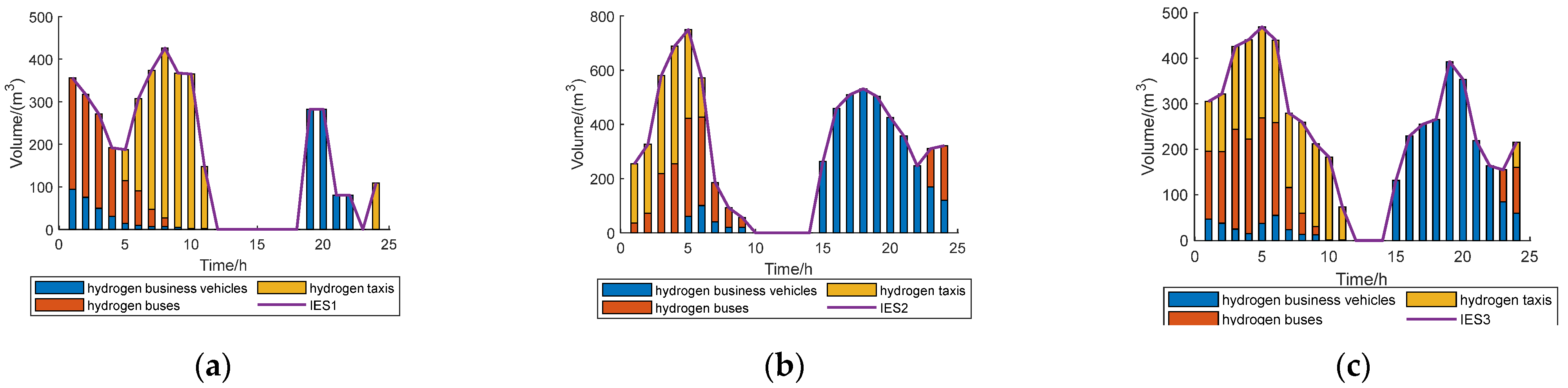
The scheduling cycle of a given cluster scenario encompassed 24 h, and the scheduling results for the 10 typical scenarios of IES1 in the three adjacent IESs are shown in Figure 7. In the DRE scenario depicted in Figure 5, the scenario data dispersion of IES1 was the highest, whereas the scenario data dispersion of IES2 and IES3 was low; please refer to Appendix B for the scheduling results of IES2 and IES3.
As shown in Figure 7, electric energy mainly originated from HP, DRE, HFC, GP, and energy sharing, and was mainly consumed by the P2H and electrical load. In IES1, compared with the traditional utilization mode, P2H provided 86.91% of the oxygen supply instead of VPSA, and the provided hydrogen energy was interactively used by the HFCs, hydrogen charging stations, and hydrogen energy systems. P2H was no longer simply a device to absorb excess renewable energy, but an energy hub for electricity, heat, oxygen, and hydrogen.
In the cluster, the HFC electricity supply was concentrated during peak load hours, and the EF electricity consumption was concentrated at night, corresponding to the heat balance. The transmission of electric energy to IES2 and IES3 was concentrated at night, and during daytime peak hours, IES2 and IES3 transmitted electric energy to IES1. In terms of heat supply, CSP, together with HFCs and EFs, flexibly adjusted the heat power. The EF and CSP models are complementary models. EFs were used to supply heat at night, CSP was used to supply heat during the day, and HFCs were used to supply heat during peak hours. With regard to the oxygen supply, P2H combined VPSA and oxygen sharing, with P2H providing the main oxygen supply and VPSA and oxygen sharing providing auxiliary oxygen supplies. Oxygen sharing in the cluster occurred as follows: IES3 sent oxygen to IES1 during the day, IES1 sent oxygen to IES3 at night, and IES2 sent oxygen to IES1 most of the time. With regard to the hydrogen supply, the hydrogen production of P2H basically remained constant. During the peak period of hydrogen demand, IES2 delivered hydrogen to IES1. In the afternoon, IES2 delivered hydrogen to IES2 by reducing hydrogen sales in the afternoon and at night. Due to the minimum hydrogen production of P2H, IES3 produced hydrogen during the middle period. IES1 delivered hydrogen to IES3 to bridge the peak period of the hydrogen demand of IES3. IES3 delivered hydrogen to IES2 to bridge the peak period of the hydrogen demand of IES2.
A comparison of the IES cluster energy supply price and market price is shown in Figure 8, and a comparison of the cluster energy supply revenue is provided in Table 11. The price fluctuations in the 10 scenarios were basically the same, so only the price of the 10th scenario was given.
According to Figure 8 and Equations (A11)–(A14), the energy supply price in the cluster should be lower than the market price based on ensuring a 10% profit, and lower prices could enhance demand-side activity. The market price of hydrogen includes the transportation price (7.79 RMB/kg), hydrogen injection price (8.73 RMB/kg), and production cost (25 RMB/kg). The price of hydrogen in the cluster is the pipeline transportation cost. Only the transportation cost of the booster station and the cost after P2H allocation should be considered. The hydrogen supply object is the hydrogen charging station.
As indicated in Table 11, the electricity price in the cluster was the median value of the electricity purchase and sale price of the cluster. The market price to purchase electricity accounts for 0.66 kWh/RMB of the electricity price in Lhasa. The market price of heating income includes the income of natural gas heating (G) and electric heating €. Although the total income of the cluster under the 10 scenarios was lower than the market price income, the pricing mechanism in the cluster maintained a 10% profit, which did not reduce the interests of the IES cluster.

4.3.2. Equipment Effect Analysis

To verify the effect of the P2H oxygen supply, CSP, and demand response, a comparison of relevant cases was performed, as summarized in Table 12. Table 13 provides the specific optimization results without CSP in Case 3, and Table 14 lists the specific optimization results for the P2H oxygen supply in Case 6. Table 15 provides the total number of IES cluster demand responses under the 10 scenarios.
Compared with Case 3, the operation cost in Case 1 was reduced by 12.88%. Without CSP, the impact on cluster cost optimization was the greatest. Compared with the specific results provided in Table 9, the electricity purchase and sale cost, hydrogen purchase and sale cost, and demand response cost of the cluster increased. Compared with Case 6, the operating cost in Case 1 was reduced by 7.26%. Without the P2H oxygen supply, the P2H energy consumption was reduced, and the electricity purchase and sale cost of the cluster were reduced, but the hydrogen purchase and sale cost increased. As there was no P2H oxygen supply, the cost of P2H could not be shared, and the oxygen supply and hydrogen sale prices increased, which reduced the enthusiasm on the demand side from Case 1 levels. Compared with Case 2, the operation cost in Case 1 was reduced by 6.55%. Compared with Cases 3 and 6, the impact was minimal without the demand response.
The CSP and CSP-HS scheduling processes in Scenario 10 were used to analyze the effectiveness of CSP, as shown in Figure 9 and Figure 10, respectively. Figure 9 shows that with the help of the CSP high-density heat tank, the CSP delayed the period of heating and power generation, further improving cluster flexibility. In terms of the electricity supply, cooperation with other equipment in the power supply was realized to simultaneously cut peaks and bridge valleys; in terms of the heat supply, HFCs were used to supply the peak heat load in coordination with EFs and HFCs, and EFs and CSP were used to provide the remainder.
Comparing Figure 7 and Figure A1 in Appendix B and Table 16, it is evident that, compared with Case 1, part of the oxygen load in IES1in Case 6 was supplied by P2H, replacing 78.39% of the VPSA oxygen supply. A total of 81,505.68 kW of electricity was saved under the 10 scenarios. In IES2, under the combined P2H-VPSA oxygen supply, the output of P2H basically remained stable, replacing 65.22% of the VPSA oxygen supply and saving 53,180.39 kW of electricity under the 10 scenarios. In IES3, under the combined P2H-VPSA oxygen supply, the output of P2H basically remained constant, replacing 42.88% of the VPSA oxygen supply, and 54,963.07 kW of electricity was saved under the 10 scenarios.

4.3.3. Multiple Energy Sharing Analysis

In a conventional IES, when DRE cannot be consumed in real time, energy is discarded, and the absorption rate of DRE is reduced. Therefore, the energy sharing mode was adopted and hydrogen and oxygen sharing was assessed. To verify the advantages of multiple energy sharing, Table 17 provides a comparison of three scenarios, and the specific results are as follows: compared with Case 4 (oxygen sharing), the cost of IES1 in Case 1 decreased by 0.9%, the cost of IES2 decreased by 10.3%, and the cost of IES3 increased by 6.3%. Case 5 (hydrogen sharing) was similar to Case 4, and compared with Cases 4 and 5, the total cost decreased by 1.61 and 3.99%, respectively. Combined with Figure 7 and Figure A1, the results show that in hydrogen or oxygen sharing, IES3 was mainly responsible for the transmission of hydrogen and oxygen from IES1 to IES2. This occurred because the generation capacity of DRE was the main impact factor of multiple energy sharing. Overall, the DRE generation capacity decreased, and under the multiple energy sharing mode, the overall economy of the IES cluster improved.

4.3.4. Different Confidence Levels for Cluster Result Comparison

In DRO, different confidence levels could yield varying degrees of conservatism of the cluster. In this paper, we analyzed the model calculation results by setting different confidence intervals. The parameter settings are listed in Table 18. Regarding the conservative responses of uncertain systems, the higher the system cost, the higher the degree of conservatism, and the lower the risk preference and the higher the adjusted reserve capacity of the system, to balance the larger error and higher energy consumption of the DRE output. However, considering the high uncertainty in DRE in Tibet, we selected the most conservative of the defined confidence levels in this paper.
Furthermore, the 1 norm with α 1 = 0.2 ,   0.5 , 0.9 and the norm with α = 0.5 , 0.9 , 0.99 were selected for comparison with the double-norm constraints, as summarized in Table 19 and Table 20, respectively. The results indicate that, at the same confidence level, the operation costs under the double-norm constraints were lower than under single-norm constraints.

5. Conclusions

In this study, considering multiple energy sharing and multi-energy coupling, a DRO model of IES clusters was built. The DRO method based on double-norm constraints was introduced to address the uncertainty in DRE. The main conclusions are as follows:
(1)
Based on the demand for a dispersed oxygen supply and energy development planning in the plateau region, an IES was built by coupling electricity, heat, oxygen, and hydrogen. Considering the current energy situation in Tibet and the emission peak and carbon neutrality targets of China, the traditional IES was improved by introducing clean energy units to achieve extremely low carbon emissions and improve DRE consumption levels. The enthusiasm on the demand side was enhanced through a reasonable pricing mechanism without reducing the cluster profit level. The scenario comparison showed that the cluster economy was higher than in other scenarios.
(2)
DRO optimization under double-norm constraints achieved a better balance between robustness and economy. Therefore, DRO was more effective in addressing the uncertainty in the DRE output in IES cluster optimization. At the same time, the two confidence intervals of the double-norm constraints were parameters reflecting the decision-maker’s risk preference. The lower the degree of conservatism, the lower the operating cost and the higher the benefits of the double-norm constraint strategy. Decision-makers must choose different confidence intervals according to their risk preferences.
(3)
The multiple energy sharing mechanism of the IES cluster provided a higher economic advantage than that provided by the single electricity sharing mechanism. Due to the various energy consumption habits and DRE installation levels of each IES, the energy consumption in each IES may considerably vary, which may lead to an energy surplus and energy waste. However, the multiple energy sharing mechanism solved this problem. The scenario comparison revealed that the multiple energy sharing mechanism effectively reduced the cluster cost, planned capacity, and energy storage usage.
To satisfy energy sharing among clusters and the interconnection with electricity and hydrogen markets, multi-energy sharing mechanisms were used in this study to make connections among multiple regional IESs. Although the demand for a dispersed oxygen supply is unique to plateau areas, oxygen is widely used in situations such as oxygen-rich combustion and medical care. Therefore, this model can have generalizable value. The DRO model sets the energy interaction price of adjacent IESs as the energy supply price. Energy sharing price design should be considered in the future to further enhance the economic benefits of the cluster. Furthermore, it is vital to consider energy network optimization (electricity, hydrogen, and heat) in the optimization of multi-energy systems to ensure the feasibility of the obtained dispatch solutions. Therefore, research on energy network optimization should be the focus of future work.

Author Contributions

Conceptualization, R.Z.; methodology, S.C.; software, S.C.; validation, Y.G. and S.C.; formal analysis, S.C.; investigation, S.C.; resources, R.Z.; data curation, S.C.; writing—original draft preparation, S.C.; writing—review and editing, R.Z.; visualization, S.C.; supervision, R.Z.; project administration, Y.G.; funding acquisition, the National Natural Science Foundation of China. All authors have read and agreed to the published version of the manuscript.

Funding

This research was funded by [the National Natural Science Foundation of China] grant number [52167015].

Data Availability Statement

The study did not report any data.

Conflicts of Interest

The authors declare no conflict of interest.

Appendix A

  • The other equipment constraints can be expressed as follows:
{ P H P min P H P t M H P Δ P H P l p P H P t P H P t 1 Δ P H P u p P E F . h t = η E F P E F . e t P E F . e min P E F . e t M E F Δ P E F . e l p P H P t P E F . e t 1 Δ P E F . e u p
where, P H P min denotes the lower power limit of HP, M H P denotes the HP installed capacity, Δ P H P u p and Δ P H P l p denote the HP limits of climbing power, η E F denotes the heat supply of EFs, P E F . e min denotes the lower power limit of EFs, M E F denotes the EF installed capacity, and Δ P E F . e u p and Δ P E F . e l p denote the EF limits of climbing power.
2.
Demand response
(1)
The limit of the adjustable oxygen load can be obtained as follows:
O c u t min O c u t t O c u t max
where O c u t t denotes the adjustable oxygen load volume and O c u t max and O c u t min denote the limits of the adjustable oxygen load volume.
The oxygen load after the demand response can be calculated as follows:
V O L . D R t = O L t O c u t t
(2)
The limit of the transferable electrical load can be determined as follows:
{ μ P P L t P t r t μ P P L t t = 1 24 P t r t = 0
where P t r t denotes the transferable electrical load power, μ P denotes the percentage of the translatable electrical load in the electrical load, and P L t denotes the electrical load.
The limit of the adjustable electrical load can be expressed as follows:
P c u t min P c u t t P c u t max
where P c u t t denotes the adjustable electrical load power and P c u t max and P c u t min denote the limits of the adjustable electrical load power.
The electrical load after the demand response can be obtained as follows:
P E L . D R t = P L t + P t r t P c u t t
(3)
The limit of the transferable heat load can be calculated as follows:
{ μ H H L t H t r t μ H H L t t = 1 24 H t r t = 0
where H t r t denotes the transferable heat load power, μ H denotes the percentage of the translatable heat load in the heat load, and H L t denotes the heat load.
The limit of the adjustable heat load can be expressed as follows:
H c u t min H c u t t H c u t max
where H c u t t denotes the adjustable heat load power and H c u t max and H c u t min denote the limits of the adjustable heart load power.
The heat load after the demand response can be obtained as follows:
P H L . D R t = H L t + H t r t H c u t t
3.
The HGS constraints can be expressed as follows:
{ S h s t = S h s t 1 + η s h c h V h s . c h t V h s . d i s t / η s h d i s   S h s min S h s t M h s i V h . c h min V h s . c h t α h . c h V h . c h max V h . d i s min V h s . d i s t α h . d i s V h . d i s max α h . d i s + α h . c h 1 S h s t = 1 = S h s t = 24 ( 2 t 24 )
where S h s t denotes the HGS capacity, M h s i denotes the HGS installed capacity, S h s min denotes the lower limit of the HGS capacity, α h . d i s denotes the discharging hydrogen status parameters, α h . c h denotes the charging hydrogen status parameters, V h . c h max and V h . c h min denote the limits of the charging hydrogen volume, V h . d i s max and V h . d i s min denote the limits of the discharging hydrogen volume, η s h c h denotes the charging hydrogen efficiency, and η s h d i s denotes the discharging hydrogen efficiency.
4.
IES cluster energy supply price
Through Equations (A11)–(A14), the P2H cost can be apportioned to the P2H hydrogen and P2H oxygen supplies. HFCs can be divided into power and heat supplies, and the intra-cluster electricity price is the average electricity purchase and sale price. As the hydrogen purchase cost is included in the operating cost, the hydrogen price only considers the transmission cost and cost of hydrogen energy sharing.
(1)
The heat supply price can be obtained as follows (hydrogen shares 60% of the P2H power consumption cost, and the profit is 10%):
{ P r i . h o t = 1.1 ( P C S P . H t P r i . C S P + G s e l l t P E F . e t + w h w h . e E P 2 H . H 2 ) / ( P C S P . H t + P E F . H t + P H F C . H t ) η H = V H F C . H t / V E L . H t E P 2 H . H 2 = G s e l l t V H F C . H t P H . e ρ H / η P 2 H / η H
where w h denotes the P2H cost allocation weight, which is 0.6; G s e l l t denotes the electricity sale price; E P 2 H . H 2 denotes the power consumption cost for P2H hydrogen production; w h . e denotes the real-time thermoelectric proportion of HFCs; and P r i . C S P denotes the CSP heat supply price.
(2)
The oxygen supply price can be determined as follows (the profit is 10%):
P r i . o = 1.1 G s e l l t ( V V P S A t P V P S A . e / η V P S A + w o E P 2 H . O 2 ) / ( V V P S A t + V E L . O t )
E P 2 H . O 2 = G s e l l t V E L . O t P O . e ρ O / η P 2 H
where w o denotes the P2H oxygen supply cost allocation weight, which is 0.6; E P 2 H . O 2 denotes the power consumption cost for P2H oxygen production; and the value is the same as that of E P 2 H . H 2 .
(3)
The hydrogen supply price can be obtained as follows (the profit is 10%):
P r i . H 2 = P r i . t r a n + 1.1 ( 1 w 0 ) E P 2 H . H 2 / V E L . h t
where P r i . t r a n denotes the price of hydrogen pipeline transportation, at 10.73 RMB/kg.
Table A1. Initial scenario probability.
Scenario 1Scenario 2Scenario 3Scenario 4Scenario 5Scenario 6Scenario 7Scenario 8Scenario 9Scenario 10
IES10.170.100.090.110.070.090.050.120.120.08
IES20.070.050.120.040.060.040.070.050.310.09
IES30.060.10.120.160.090.080.080.060.090.16

Appendix B

Figure A1. IES2 and IES3 energy balance. (a) IES2 and IES3 electric power balance. (b) IES2 and IES3 heat power balance. (c) IES2 and IES3 oxygen balance. (d) IES2 and IES3 hydrogen balance.
Energies 15 08723 g0a1Energies 15 08723 g0a2

References

  1. GB/T 35414-2017; Requirements of Oxygen Conditioning for Indoor Oxygen Diffusion in Plateau Area. The Standardization Administration of China: Beijing, China, 2017.
  2. DJB 540005-2018; Specification for Engineering Construction and Acceptance of Civil Oxygen Supply in Tibet. Department of Housing and Urban Rural Development of the Tibet Autonomous Region: Tibet, China, 2018.
  3. DJB 540004-2018; Design Standard for Engineering of Civil Oxygen Supply in Tibet. Department of Housing and Urban Rural Development of the Tibet Autonomous Region: Tibet, China, 2018.
  4. Zhang, L.; Chen, L.; Zhu, W.; Lyu, L.; Cai, G.; Hai, K.L. Research on the optimal allocation method of source and storage capacity of integrated energy system considering integrated demand response. Energy Rep. 2022, 8, 10434–10448. [Google Scholar] [CrossRef]
  5. Zhang, X.; Chan, K.W.; Wang, H.; Hu, J.; Zhou, B.; Zhang, Y.; Qiu, J. Game-theoretic planning for integrated energy system with independent participants considering ancillary services of power-to-gas stations. Energy 2019, 176, 249–264. [Google Scholar] [CrossRef]
  6. Zhang, R.; Jiang, T.; Li, G.; Chen, H.; Li, X.; Ning, R.X. Bi-level Optimization Dispatch of Integrated Electricity-natural Gas Systems Considering P2G for Wind Power Accommodation. Proc. CSEE 2018, 38, 5668–5678+5924. [Google Scholar]
  7. Zhang, T.; Ma, J.; Yan, X.; Huang, W.; Wang, L.; Xu, S.; Zhang, X. Strategy optimization for virtual power plant complied with power to gas operation model. J. Phys. Conf. Ser. 2021, 2005, 012146. [Google Scholar] [CrossRef]
  8. Nsafon, B.E.K.; Butu, H.M.; Owolabi, A.B.; Roh, J.W.; Suh, D.; Huh, J.-S. Integrating multi-criteria analysis with PDCA cycle for sustainable energy planning in Africa: Application to hybrid mini-grid system in Cameroon. Sustain. Energy Technol. Assess. 2020, 37, 100628. [Google Scholar] [CrossRef]
  9. Viola, P.; Jones, M. Rapid Object Detection using a Boosted Cascade of Simple. In Proceedings of the 2001 IEEE Computer Society Conference on Computer Vision and Pattern Recognition (CVPR 2001), Kauai, HI, USA, 8–14 December 2001. [Google Scholar]
  10. Li, Y.; Meng, F.; Chen, Y.; Wu, Y.; Wangdang, D. Research and development Status of oxygen production technology in the Tibet. Low Temp. Spec. Gases 2021, 39, 5–9, 31. [Google Scholar]
  11. Ran, Z.; Luo, Y. Research progress of oxygen production and supply technology and rational use of oxygen at high altitude. People’s Mil. Surg. 2019, 62, 66–470. [Google Scholar]
  12. Li, W.; Yu, B.; Tian, G.; Zhao, H. Design of diffused oxygen supply scheme in plateau area. Med. Gases Eng. 2018, 3, 15–17. [Google Scholar]
  13. Gregoratti, D.; Matamoros, J. Distributed Energy Trading: The Multiple-Microgrid Case. IEEE Trans. Ind. Electron. 2015, 62, 2551–2559. [Google Scholar] [CrossRef] [Green Version]
  14. Chen, J.; Köbis, E.; Yao, J.-C. Optimality Conditions and Duality for Robust Nonsmooth Multiobjective Optimization Problems with Constraints. J. Optim. Theory Appl. 2019, 181, 411–436. [Google Scholar] [CrossRef]
  15. Siqin, Z.; Niu, D.; Li, M.; Gao, T.; Lu, Y.; Xu, X. Distributionally robust dispatching of multi-community integrated energy system considering energy sharing and profit allocation. Appl. Energy 2022, 321, 119202. [Google Scholar] [CrossRef]
  16. Du, W.; Zhong, W.; Tang, Y.; Du, W.; Jin, Y. High-Dimensional Robust Multi-Objective Optimization for Order Scheduling: A Decision Variable Classification Approach. IEEE Trans. Ind. Inf. 2019, 15, 293–304. [Google Scholar] [CrossRef] [Green Version]
  17. Lei, G.; Bramerdorfer, G.; Ma, B.; Guo, Y.; Zhu, J. Robust Design Optimization of Electrical Machines: Multi-Objective Approach. IEEE Trans. Energy Convers. 2021, 36, 390–401. [Google Scholar] [CrossRef]
  18. Wei, H.-Z.; Chen, C.-R.; Li, S.-J. Characterizations for Optimality Conditions of General Robust Optimization Problems. J. Optim. Theory Appl. 2018, 177, 835–856. [Google Scholar] [CrossRef]
  19. Chen, Z.; Yu, P.; Haskell, W.B. Distributionally robust optimization for sequential decision-making. Optimization 2019, 68, 2397–2426. [Google Scholar] [CrossRef]
  20. Bertsimas, D.; Sim, M.; Zhang, M. Adaptive Distributionally Robust Optimization. Manag. Sci. 2019, 65, 604–618. [Google Scholar] [CrossRef] [Green Version]
  21. Chen, Z.; Sim, M.; Xu, H. Distributionally Robust Optimization with Infinitely Constrained Ambiguity Sets. Oper. Res. 2019, 67, 1328–1344. [Google Scholar] [CrossRef] [Green Version]
  22. Dou, X.; Anitescu, M. Distributionally robust optimization with correlated data from vector autoregressive processes. Oper. Res. Lett. 2019, 47, 294–299. [Google Scholar] [CrossRef] [Green Version]
  23. Zhao, C.; Jiang, R. Distributionally Robust Contingency-Constrained Unit Commitment. IEEE Trans. Power Syst. 2017, 33, 94–102. [Google Scholar] [CrossRef]
  24. Zheng, X.; Chen, H.; Xu, Y.; Li, Z.; Lin, Z.; Liang, Z. A Mixed-integer SDP Solution to Distributionally Robust Unit Commitment with Second Order Moment Constraints. CSEE J. Power Energy Syst. 2020, 6, 374–383. [Google Scholar]
  25. Dong, S.; Wang, S.; Lin, Z.; Jian, X.; Sun, F.; Sun, H. Distributed Robust Optimization of Integrated Energy System Considering Integrated Demand Response. J. Phys. Conf. Ser. 2021, 1972, 012017. [Google Scholar] [CrossRef]
  26. Li, P.; Song, L.; Qu, J.; Huang, Y.; Wu, X.; Lu, X.; Xia, S. A Two-Stage Distributionally Robust Optimization Model for Wind Farms and Storage Units Jointly Operated Power Systems. IEEE Access 2021, 9, 111132–111142. [Google Scholar] [CrossRef]
  27. Zhang, S.; Zhang, D.; Qiao, J.; Zhang, Z. Preventive control for power system transient security based on XGBoost and DCOPF with consideration of model interpretability. CSEE J. Power Energy Syst. 2021, 7, 279–294. [Google Scholar]
  28. Wang, L.; Jiang, C.; Gong, K.; Si, R.; Shao, R.; Liu, W. Data-driven distributionally robust economic dispatch for distribution network with multiple microgrids. IET Gener. Transm. Distrib. 2020, 14, 5712–5719. [Google Scholar] [CrossRef]
  29. Ding, T.; Yang, Q.; Yang, Y.; Li, C.; Bie, Z.; Blaabjerg, F. A Data-Driven Stochastic Reactive Power Optimization Considering Uncertainties in Active Distribution Networks and Decomposition Method. IEEE Trans. Smart Grid 2018, 9, 4994–5004. [Google Scholar] [CrossRef]
Figure 1. IES architecture.
Energies 15 08723 g001
Figure 2. Multi-energy sharing architecture.
Energies 15 08723 g002
Figure 3. Flow chart of the model optimization process.
Energies 15 08723 g003
Figure 4. IES1 (a), IES2 (b), and IES3 (c) loads.
Energies 15 08723 g004
Figure 5. DRE of IES1 (a), IES2 (b), and IES3 (c).
Energies 15 08723 g005
Figure 6. IES cluster charging hydrogen prediction for HICEVs, IES1 (a), IES2 (b), and IES3 (c).
Energies 15 08723 g006
Figure 7. IES1 energy balance. (a) IES1 electric power balance. (b) IES1 heat power balance. (c) IES1 oxygen balance. (d) IES1 hydrogen balance.
Energies 15 08723 g007
Figure 8. IES cluster energy supply and market prices. (a) Heat price. (b) hydrogen price. (c) Oxygen price.
Energies 15 08723 g008
Figure 9. CSP scheduling results of IES1 (a), IES2 (b), and IES3 (c).
Energies 15 08723 g009
Figure 10. CSP-HS scheduling results of IES1 (a), IES2 (b), and IES3 (c).
Energies 15 08723 g010
Table 1. Oxygen load-related parameters.
Unit (W/m2)
IES1IES2IES3
η e . a 225300330
η h . a 809080
Table 2. Purchase and sale price of the power grid.
Time/(h)
1–78–1112–1415–1819–2223–24
Purchase/RMB0.40.751.20.751.20.4
Sale/RMB0.20.40.60.40.60.2
Table 3. Relevant parameters.
EquipmentComprehensive CostEfficiencyEnergy Consumption RatioClimbing Power
(Polymer electrolyte membrane (PEM)) P2H10,000 (RMB/kW)0.735 (kW/kg)20%
HFC1000 (RMB/kW)0.953.3 (kW/Nm3)20%
VPSA4500 (RMB/kW)0.850.45 (kW/Nm3)20%
HP12,000 (RMB/kW)//20%
WT22,000 (RMB/kW)///
PV9600 (RMB/kW)///
HGS3000 (RMB/kg)0.95/250 (Nm3/h)
Table 4. CSP.
Table 4. CSP.
EquipmentComprehensive CostEfficiencyHeated Fluid TransmissionClimbing Power
CSP30,000 (RMB/kW)0.8 (electric)0.7220%
HS0.95/2000 (kW/h)
Table 5. CSP installed capacity.
EquipmentInstalled Capacity/(MW)
IES1IES2IES3
CSP P C S P 1 . e max P C S P 2 . e max P C S P 3 . e max
HS101010
Table 6. Pipeline and hydrogen charging station parameters.
Oxygen Transmission PipelineHydrogen Transmission PipelineHydrogen Charging Stations
Cost500,000 (RMB/km)630,000 (dollar/km)3 × 5 million
Length/(km)3 × 103 × 10/
Table 7. Case set.
Table 7. Case set.
Case 1Case 2Case 3Case 4Case 5Case 6Case 7Case 8
DR ×
CSP ×
Oxygen sharing ×
Hydrogen sharing ×
P2H ×
1 − norm ×
∞ − norm ×
Table 8. Equipment planned capacity.
VPSA
/(kW)
P2H
/(kW)
EF
/(kW)
HP
/(kW)
HGS
/(m3)
HFC
/(kW)
IES1121.634931.432453.755772.991640.153378.40
IES2150.492236.971427.282945.4815001186.28
IES3683.732793.841572.924035.4710001331.90
Table 9. Model optimization results.
Cost/(RMB)Abandonment DRE Rate R D R E  
10 × f b r   f e i   f h i   f D R i   f D R E i   f E S i   Total Cost
IES1195,254.30−79,402.76−230,194.491466.54019,874.013,369,750.5040.02%
IES2110,220.13−73,772.37−243,107.03999.13020,695.12037.79%
IES3119,101.72−60,178.25−253,665.723389.98017,885.06042.76%
Table 10. Multi-energy sharing.
Electricity Sharing/(kW)Volume/(m3)
Oxygen SharingHydrogen Sharing
1 to 250,407.581939.3425,911.81
2 to 157,586.2387,531.0753,536.94
2 to 348,736.95862.846008.74
3 to 251,212.0740,071.9387,791.24
1 to 358,749.58100,320.4084,184.06
3 to 154,415.7259,353 217527.67
Table 11. Energy supply income.
Income/(RMB)
Electricity SupplyHeat SupplyOxygen SupplyHydrogen Supply
Market price1,645,868.40961,179.10 (G)1,185,047.03705,210.02
921,750.00 (E)
IES cluster price1,552,777.50537,174.10317,194.00308,350.30
Table 12. Comparison of the results of Cases 1–3 and 6.
Cost/(RMB)
Case 1Case 2Case 3Case 6
IES11,664,286.001,680,287.081,935,782.591,670,702.04
IES2807,016.30886,898.42981,657.05948,911.43
IES3898,448.201,038,758.88950,317.001,013,862.14
Table 13. Case 3 results.
Cost/(RMB)
10 ×   f b r
f e i
f h i
f D R i
f D R E i
f E S i
IES11,945,546.92154,771.28−170,195.813457.9602202.24
IES21,218,976.59−42,413.58−197,561.301488.7801166.56
IES31,164,351.28−36,194.57−183,101.664144.4701117.48
Table 14. Case 6 results.
Cost/(RMB)
10 ×   f b r
f e i
f h i
f D R i
f D R E i
f E S i
IES11,945,546.92−91,629.17−206,761.482239.84019,643.03
IES21,218,976.59−89,677.82−210,365.621071.29021,161.27
IES31,164,351.28−74,542.60−206,665.403322.16018,084.26
Table 15. IES1 DR.
Table 15. IES1 DR.
Electrical Load Response/(kW)Volume/(m3)
Heat Load ResponseOxygen Load Response
IES1134,012.082,905.070,588.29
IES268,319.0049,354.5025,713.35
IES347,043.0045,667.0033,216.26
Table 16. Percentage of the P2H oxygen supply in the combined P2H-VPSA oxygen supply.
IES1IES2IES3
Percentage (%)78.3965.2242.88
Table 17. Comparison of the results of Cases 1, 4, and 5.
Cost/(RMB)
Case 1Case 4Case 5
IES11,664,286.001,680,196.641,694,205.04
IES2807,016.30899,993.33924,279.15
IES3898,448.20844,621.54891,407.86
Table 18. Comparison of the results at different confidence levels.
α 1   α  
0.50.90.99
0.203,325,749.923,330,083.263,336,340.05
0.503,329,127.753,333,823.713,369,750.50
0.903,320,367.903,337,569.983,349,257.23
Table 19. Comparison of the results of Cases 1 and 8.
Double Norm1 − Norm
0.203,336,340.053,432,631.62
0.503,369,750.503,434,569.65
0.903,349,257.233,468,672.31
Table 20. Comparison of the results of Cases 1 and 7.
Double Norm∞ − Norm
0.503,336,340.053,430,380.45
0.903,369,750.503,445,127.40
0.993,349,257.233,446,824.83
Publisher’s Note: MDPI stays neutral with regard to jurisdictional claims in published maps and institutional affiliations.

