Tuning Model Predictive Control for Rigorous Operation of the Dalsfoss Hydropower Plant

Abstract

Model predictive control is considered an attractive control strategy for the operation of hydropower station systems. It is due to the operational constraints or requirements of the hydropower system for safe and eco-friendly operation. However, it is mandatory to tune the model predictive control to achieve its best and most efficient performance. This paper determines the appropriate tunning on the weight parameters and the length of the prediction horizon for implementing model predictive control on the Dalsfoss hydropower system. For that, several test sets of the weight parameter for the optimal control problem and different lengths of the prediction horizon are simulated and compared.

1. Introduction

As global warming has become a severe problem, the world has been trying to reduce the use of fossil fuels. Renewable energy has been spotlighted as the key technology to mitigating the emission of greenhouse gas. Renewable energy has been actively adopted globally for the green shift [1].

Hydropower plays an essential role in the green shift. It is because hydropower is the only renewable technology that can provide energy on demand. Most of the other renewable technologies, e.g., solar and wind, can generate power intermittently depending on the weather conditions. Despite the advantages of hydropower, its operation is challenging owing to strict operational constraints. The operational constraints are to prevent damage to the environment and residents around watercourses and reservoirs. For example, the change of the discharged water flowrate from the hydropower plant must be inhibited as much as possible to keep the fauna and the resident environments safe along the water course [2,3].

The complicated operational requirements make model predictive control (MPC) an appealing control approach for the operation of hydropower. MPC is a control approach that computes control input sequences for the future by solving a finite horizon open-loop optimal control problem (OCP) based on the current state and given information of the system as the initial point. Then, the first control input in the control sequence is applied and this process repeats in every sampling time. In other words, MPC has the capability to deal with a dynamic system with multiple inputs, outputs, and constraints [4,5,6].

There has been a series of studies on the implementation of MPC in the Dalsfoss hydropower plant system. The Dalsfoss hydropower plant is an impoundment type of hydropower plant that is located uppermost in the Kragerø watercourse [7,8]. The operation of the Dalsfoss hydropower plant must comply with the constraints that NVE regulated, e.g., the water level, the change of discharged flowrate, and the minimum flowrate of discharged water [9]. There was an initial attempt to simulate MPC on the Dalsfoss hydropower plant. This work suggested the model of the system and formulated the reference tracking OCP to keep the water level within a specific range. By keeping the buffer space in the reservoir, this MPC obtained the capability to deal with the system uncertainties [10]. A model was updated with new parameters after the severe mismatch between the model and the reality was found during a flood in September 2015 [11]. For better operation under the uncertainty of water inflow forecast, multi-objective optimization(MOO) MPC was implemented with the reference region tracking OCP [12]. Then, the new OCP that maximizes the water level in the reservoir was suggested and compared to the conventional OCP. Although the new OCP gives the advantage of not wasting water at the reservoir, it shows a weakness in the robustness of the constraint satisfaction under the presence of the system uncertainty [13]. This robustness problem was solved by adopting multi-stage MPC [14].

Although there has been a series of research on using MPC for the operation of the hydropower station, parameter tuning for the rigorous operation has not been performed yet. Therefore, this work aims to tune MPC for operating hydropower safely and eco-friendly with minimized computational demand. To determine the appropriate tunning of MPC for the rigorous operation, four test sets (including the conventional setting) and seven different lengths of prediction horizons (including the conventional setting) are used for the simulations. Furthermore, for a more realistic simulation, the historically stored actual data of the water inflow and the power production are applied. By comparing the simulation results, the proper tuning of weight parameters and the appropriate length of prediction horizon are obtained.

This paper is organized as follows: Section 2 explains the system model, operational constraints, and optimal control problem. Section 3 presents simulation settings such as test sets of parameters and simulation conditions. The result is presented in Section 4 and the conclusion is made in Section 5.

2. System Description

2.1. System Model

The Dalsfoss hydropower plant is operated by using water from its reservoir, lake Toke. For the effective and efficient operation of the hydropower plant, it is important to control the level of the reservoir. Figure 1 shows the simplified layout of the reservoir. The reservoir, lake Toke, is divided into two parts. The left side of Figure 1 depicts the upper part of the reservoir, called Merkebekk, and the right side describes the lower part of the reservoir, called Dalsfoss, which is near the dam and the plant. The water inflows into the reservoir, ${\dot{V}}_i$ [m${}^3$/s] come from various sources such as precipitation and ice-melting. A certain proportion, $\beta$, of the water inflow, goes into Dalsfoss and the rest goes into Merkebekk. The water is discharged through floodgate, ${\dot{V}}_{\mathrm{g}}$ [m${}^3$/s], and turbine, ${\dot{V}}_{\mathrm{t}}$ [m${}^3$/s]. The system model of lake Toke is derived in [10] as follows:

Figure 1. Schematic of lake Toke [10].

There are two states in the system. One is the water level at Merkebekk and the other is the water level at Dalsfoss, denoted as $h_1$ [m] and $h_2$ [m] respectively. Both states are measurable and observable. $x_M$ [m MSL] and $x_D$ [m MSL] mean the water level above the sea level (m MSL) at Merkebekk and Dalsfoss. They are calculated as:

$$x_{\mathrm{M}}=h_1+x_{\mathrm{LRV}}^{\min }$$

(1)

$$x_{\mathrm{D}}=h_2+x_{\mathrm{LRV}}^{\min }$$

(2)

where $x_{\mathrm{LRV}}^{\min }$ [m MSL] means the low regulated value of the water level.

Due to the curvature shape of the lake, the area of the lake surface changes depending on the water level at lake Toke. The minimum area of the lake surface is specified as $28\times {10}^6$ m${}^2$. Therefore, the area of the lake according to the water level, $A\left(h_i\right)$ [m${}^2$], is computed as:

$$A\left(h_i\right)=max(28\times {10}^6·1.1·h_i^{\frac{1}{10}},{10}^3)$$

(3)

The area of lake toke can be divided into the areas of Dalsfoss and Merkebekk based on the proportion, $\alpha$.

The flow from Merkebekk to Dalsfoss denoted as ${\dot{V}}_{12}$ [m${}^3$/s], is calculated based on the height difference of the water levels at both places as follows:

$${\dot{V}}_{12}=K_{12}·(h_1-h_2)\sqrt{|h_1-h_2|}$$

(4)

where $K_{12}$ is the flow coefficient in lake Toke.

Two control inputs in the system are the opening heights of two floodgates at the reservoir. The structure of the floodgate is shown in Figure 2. The floodgate opens upwards. Therefore, the minimum value of water level at Dalsfoss, $h_2$, or the opening height of the floodgate, $h_{\mathrm{g}i}$ is used to calculate the flowrate through the floodgate. The floodgate is located above the low regulated value of the water level, $x_{\mathrm{LRV}}^{\min }$. When the water level at Dalsfoss, $h_2$ is lower than the low regulated value of the water level, $x_{\mathrm{LRV}}^{\min }$, the water does not flow out through floodgate. The opening heights on floodgates are denoted as $h_{\mathrm{g}1}$ and $h_{\mathrm{g}2}$. The openings of floodgates and the level of the water at Dalsfoss determine the amount of water thrown out through floodgates, ${\dot{V}}_{\mathrm{g}}$ [m${}^3$/s], as:

$${\dot{V}}_{\mathrm{g}}=C_{\mathrm{d}}·w·min(h_{\mathrm{g}},h_2)\sqrt{2g·max(h_2,0)}$$

(5)

where $C_{\mathrm{d}}$ is the discharge coefficient and g is the acceleration of gravity. The width of the floodgate is denoted as w. The maximum opening height of floodgates is limited by $5.6$ m.

Figure 2. Structure of floodgate [10].

The power production plan is denoted as ${\dot{W}}_{\mathrm{e}}$ [MW] and it is decided by optimization based on many factors such as water level, price, demand, etc by Skagerak. The water flowrate through a turbine, ${\dot{V}}_{\mathrm{t}}$ [m${}^3$/s], is determined by how much power must be generated according to the power production plan as:

$${\dot{V}}_{\mathrm{t}}=a\frac{{\dot{W}}_{\mathrm{e}}}{x_{\mathrm{D}}-x_{\mathrm{q}}}+b$$

(6)

In Equation (6), $x_{\mathrm{q}}$[m] means the water level at the quay where the water is discharged. a and b indicate parameters obtained from the data fitting method. The water level at the quay is calculated by solving the following cubic equation:

$$\begin{array}{cc}\hfill 0& =c_1{x}_{\mathrm{q}}^3+(c_2-c_1{x}_{\mathrm{D}})x_{\mathrm{q}}^2\hfill \\ \hfill & +(c_3-c_2{x}_{\mathrm{D}}+c_4{\dot{V}}_{\mathrm{g}})x_{\mathrm{q}}\hfill \\ \hfill & +{\dot{W}}_{\mathrm{e}}-c_3{x}_{\mathrm{D}}-c_4{\dot{V}}_{\mathrm{g}}{x}_{\mathrm{D}}-c_5\hfill \end{array}$$

(7)

where $c_1$, $c_2$, $c_3$, $c_4$, and $c_5$ are coefficients that are obtained by the polynomial data fitting method. For this method, the historically stored data in the Dalsfoss hydropower plant are used.

The total flowrate at downstream from the Dalsfoss power station, ${\dot{V}}_{\mathrm{o}}$ [m${}^3$/s], is computed as:

$${\dot{V}}_{\mathrm{o}}={\dot{V}}_{\mathrm{t}}+\sum {\dot{V}}_{\mathrm{g}}$$

(8)

The dynamic model is described by the following equations:

$$\frac{d{h}_1}{dt}=\frac{1}{(1-\alpha )A\left(h_1\right)}((1-\beta ){\dot{V}}_{\mathrm{i}}-{\dot{V}}_{12})$$

(9)

$$\frac{d{h}_2}{dt}=\frac{1}{\alpha A\left(h_2\right)}(\beta {\dot{V}}_{\mathrm{i}}+{\dot{V}}_{12}-{\dot{V}}_{\mathrm{o}})$$

(10)

Parameters for the system model are specified in Table 1.

Table 1. Parameters for Lake Toke model.

Parameter	Value	Unit	Comment
$\alpha$	0.05	-	Fraction of surface area in compartment 2
$\beta$	0.02	-	Fraction of inflow to compartment 2
$K_{12}$	800	m${}^{\frac{3}{2}}$/s	Flow coefficient
$C_{\mathrm{d}}$	0.7	-	Discharge coefficient, Dalsfoss gate
$w_1$	11.6	m	Width of Dalsfoss gate 1
$w_2$	11.0	m	Width of Dalsfoss gate 2
$x_{\mathrm{LRV}}^{\min }$	55.75	m MSL	Minimal low regulated level value
g	9.81	m/s${}^2$	Acceleration of gravity
a	124.69	Pa${}^{-1}$	Coefficient in Equation (6)
b	3.161	m${}^3$/s	Coefficient in Equation (6)
$c_1$	0.13152	W/m${}^{-3}$	Polynomial coefficient in Equation (7)
$c_2$	−9.5241	W/m${}^2$	Polynomial coefficient in Equation (7)
$c_3$	1.7234 · 10${}^2$	W/m	Polynomial coefficient in Equation (7)
$c_4$	−7.7045 · 10${}^{-3}$	Pa/m	Polynomial coefficient in Equation (7)
$c_5$	−8.7359 · 10${}^{-1}$	W	Polynomial coefficient in Equation (7)

2.2. Operational Constraints

Several operational constraints ensure operational safety, securing ecological fauna and avoiding damages to properties around the water course and hydropower plant. The main constraints are listed below:

• The sudden change in the flowrate at downstream, ${\dot{V}}_{\mathrm{o}}$, can endanger the properties and ecosystem along the watercourse. Therefore, the flowrate at downstream must be kept as constant as possible. The change of the flowrate at downstream is desired to keep less than 50 ${\mathrm{m}}^3/\mathrm{s}$ on every time step.
• The flowrate at downstream, ${\dot{V}}_{\mathrm{o}}$, must be more than $4{\mathrm{m}}^3/\mathrm{s}$. This constraint is to ensure that fishes in downstream can move freely along the water course.
• The water level at Merkebekk, $x_{\mathrm{M}}$, must be maintained within a certain range as:

  $$x_{\mathrm{M}}\in [x_{\mathrm{LRV}},x_{\mathrm{HRV}}]$$

  where $x_{\mathrm{LRV}}$ and $x_{\mathrm{HRV}}$ mean the low and the high regulated value for the water level, respectively. The range changes seasonally as shown in Table 2.
  Table 2. Seasonal level requirement.

  Date	${\mathit{x}}_{\mathbf{LRV}}\left[\mathbf{m}\right]$	${\mathit{x}}_{\mathbf{HRV}}\left[\mathbf{m}\right]$
  1 January–30 April	55.75	60.35
  1 May–30 August	58.85	59.85
  1 September–14 September	55.75	59.35
  28 October–11 November	55.75	59.85
  12 November–31 December	55.75	60.35

• The maximum flowrate through the turbine, $V_{\mathrm{t}}$, is limited up to 36 ${\mathrm{m}}^3/\mathrm{s}$.

2.3. Optimal Control Problem

During the operation of a hydropower plant, it is desired to minimize the use of the floodgates unnecessarily and maximize the water level at the reservoir while considering operational constraints. Otherwise, it would result in loss of water which otherwise could be used to produce electricity. Therefore, to achieve the desired operation while satisfying the operational constraints, the objective function in the OCP is suggested in [13] as:

$$\underset{u}{min}\sum _{i=1}^{N_p}{\omega }_R{R}_{\mathrm{new}}^2\left(x_{t+i}\right)+{\omega }_u{u}_{\mathrm{c},t+i-1}^2+{\omega }_{\Delta u}\Delta u_{\mathrm{c},t+i-1}^2+p^2{\omega }_p$$

(11)

The first term in Equation (11) is designed to increase the water level at Merkebekk til the value of HRV and is expressed as:

$$R_{\mathrm{new}}\left(x_{t+1}\right)=x_{\mathrm{M},t+1}-x_{\mathrm{HRV}}$$

(12)

The second and third terms in Equation (11) are to minimize the use of the floodgate openings and to minimize the change of floodgate openings, respectively. $u_{\mathrm{c}}$ indicates the control action taken in open-loop optimization through the prediction horizon. $\Delta u_{\mathrm{c},t+i-1}^2$ in the third term in Equation (11) ex expressed as ${(u_{\mathrm{c},t+i-1}-u_{\mathrm{c},t+i-2})}^2$. The last term, $p^2{\omega }_p$, is the penalty for violation of level constraints. The variable, p, is the slack variable that is automatically decided by the optimizer. It is necessary to allow the violation on $x_{\mathrm{LRV}}$ to meet the minimum flowrate constraints. ${\omega }_R$, ${\omega }_u$, ${\omega }_{\Delta u}$, and ${\omega }_p$ are the weight parameters for the objective function on the OCP. If the higher value is set on a certain weight parameter, the term with the weight parameter is treated more importantly when solving the OCP. Therefore, the desired operation can be achieved.

3. Simulation Setting

This section introduces the test sets of parameters and simulation conditions to run deterministic NMPC in the Dalsfoss hydropower plant.

3.1. Test Sets of Parameters

The ideal operation of the hydropower plant is not to waste water inside of the reservoir by minimizing the use of the floodgates and keeping the water level at the reservoir as high as possible. Yet, it is important to keep the flowrate at downstream as constant as possible which is related to the change of the floodgate openings for the sake of safe and eco-friendly operation. Although the goals to achieve from the operation are known, it is impossible to obtain a set of parameters without simulations and tests. Tuning weight parameters for the implementation of MPC is often done by the trial and error method. Four test sets of weight parameters are suggested in Table 3 to run the simulation. Testset1 is the same set of the weight parameters in the conventional setting.

Table 3. Parameters of test sets for the simulations.

Parameter	Test Set 1	Test Set 2	Test Set 3	Test Set 4
${\omega }_R$	10	10	10	10
${\omega }_{\Delta u}$	1	10	100	1000
${\omega }_u$	1	1	1	1
${\omega }_p$	10,000	10,000	10,000	10,000

Due to the importance of maximizing the water level, ${\omega }_R$ is set as 10 equally. ${\omega }_p$ is set equally high as 10,000 to encourage the satisfaction of the operational constraints. ${\omega }_u$ is chosen as 1 on all the test sets. Therefore, the only variable on the test sets is ${\omega }_{\Delta u}$. It inhibits the change of the floodgate openings more when ${\omega }_{\Delta u}$ has a higher value. To show the differences in the simulations, the parameters for tests are set as 1, 10, 100, and 1000.

Various lengths of prediction horizon, N [day], are tested as:

$$N=[1,3,5,7,9,11,13]$$

(13)

Conventionally, the test set 1 and 13 days of prediction horizon are used for implementing MPC on the Dalsfoss hydropower plant. In this paper, each test set of weight parameters, shown in Table 3, is tested together with seven different lengths of prediction horizon as shown in Equation (13). Therefore, one conventional simulation and 27 other simulations are run and compared to each other to find a set of parameters for the rigorous operation of the Dalsfoss hydropower plant.

3.2. Simulation Condition

To obtain a realistic simulation result, the historically stored data of the water inflow and the power production plan are used. Figure 3 shows the historical power generation of the Dalsfoss hydropower station from 15 April 2020 to 15 May 2020. In the simulation, the perfect prediction is assumed in power production.

Figure 3. Historical power production plan during the simulation period.

The water inflow forecast is updated every 24 h. It contains how much water may flow into the reservoir for the next 13 days. The historical data from 2020 are used for simulation. Figure 4 is a water inflow forecast updated on 15 April 2020. Then, one of the ensembles is picked to run the deterministic MPC and the first value of the picked ensemble is realized in the next time step of simulation.

Figure 4. 50 ensembles of the water inflow prediction to lake Toke on 15 April 2020.

The simulation follows the order of the block diagram shown in Figure 5. The MPC optimizes the optimal control sequence based on given information of measured states $\widehat{x}$, water inflow forecast data ${\dot{V}}_i$, and power production plan ${\dot{W}}_e$. The first input of the optimal control sequence, $u^{*}$, is applied to the system with the first value of the water inflow forecast. In this simulation, the perfect model is assumed that there is no mismatch between the model and the system.

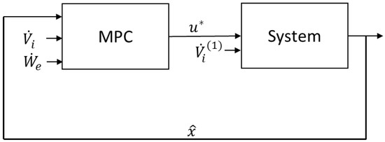
Figure 5. A block diagram of the closed of MPC.

The simulation period is set from 15 April to 15 May because this period contains a big change in the water level requirements. The IPOPT solver in CasADi is used to solve OCP [15].

4. Simulation Result

In this section, the summary of 28 simulations, the combination of four weight parameter test sets and seven lengths of prediction horizon, are presented.

Figure 6 shows the change of the water level at Merkebekk, $x_M$, and the water level bound, $x_{\mathrm{HRV}}$, during the simulation with different lengths of the prediction horizon. In labels of Figure 6, Np:i means that the length of the prediction horizon is set as i days. The upper figure describes how the water level at Merkebekk changes depending on the length of the prediction horizon when the weight parameters are set as the test set 1 (conventional setting) shown in Table 3. The lower figure displays the comparison of the water level changes with different lengths of the prediction horizon when the weight parameters are set as the test set 4 (${\omega }_{\Delta u}=1000$) in Table 3.

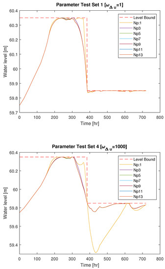
Figure 6. Change of the water level at Merkebekk during the simulations with parameter test set 1 and test set 4.

In the upper figure of Figure 6, as ${\omega }_{\Delta u}$ is set as 1 and ${\omega }_R$ is set as 10, the operation aims to maximize the water level at the reservoir. Except for when the horizon length is set as 1 day, labeled as Np:1, most of the simulations show similar results which maximize the water according to the water inflow forecast, power production plan, and the level requirement change. However, when the horizon length is set as 1 day, labeled as Np:1, the prediction horizon is so short that the water level requirement change could not be foreseen sufficiently. Therefore, a drastic water level drop is observed.

In the lower figure of Figure 6, as ${\omega }_{\Delta u}$ is set as 1000 and ${\omega }_R$ is set as 10, it aims to minimize the changes of the floodgate openings. As result, it was not prioritized to maximize the water level at the reservoir. The most of simulation results with various lengths of the prediction horizon display similar water level performance. However, when the prediction horizon length is set as 1 day, labeled as Np:1, the water level is significantly dropped at approximately 400 h where the maximum water level requirement changes.

Both figures in Figure 6 demonstrate that when the prediction horizon length is set too short as 1 day (24 h) MPC controls the system in undesirable manners. However, when the prediction horizon length is set longer than 3 days, the water level changes throughout the simulation time are quite identical.

The average water level at Merkebekk, $x_M$, from simulations with different lengths of prediction horizon, $N_{\mathrm{p}}$, and different parameter test sets are described in Table 4. The average water levels become identical on each test set of weight parameters when the prediction horizon length is longer than 7 days. Then, the average water level deviates as the prediction horizon is getting shorter. The deviation becomes bigger when the value of ${\omega }_{\Delta u}$ is higher and the prediction horizon is set as 1 day. When the length of the prediction horizon is 3 or 5 days, no big differences are found.

Table 4. Average value of water level ($h_1$) throughout simulations [m].

${\mathit{N}}_{\mathbf{p}}$ [d]	Testset 1	Testset 2	Testset 3	Test Set 4
1	4.2637	4.2625	4.2595	4.1644
3	4.2554	4.2537	4.2472	4.2314
5	4.2545	4.2528	4.2463	4.2290
7	4.2542	4.2526	4.2462	4.2294
9	4.2542	4.2526	4.2462	4.2294
11	4.2542	4.2526	4.2462	4.2294
13	4.2542	4.2526	4.2462	4.2294

Figure 7 displays the total discharged flowrate, ${\dot{V}}_{\mathrm{O}}$, from the hydropower plant depending on the test sets of the weight parameters when the prediction horizon is set as 3 days. The flowrate changes more delicately when the value of ${\omega }_{\Delta u}$ increases. It is because when ${\omega }_{\Delta u}$ is high, the optimizer compensates the high value for the change of the floodgate openings and aims to minimize it. It is beneficial to set the value of ${\omega }_{\Delta u}$ high to maintain the flowrate at downstream as constant as possible. Therefore, test set 4 shows the smoothest change of flowrate at downstream as shown in Figure 7.

Figure 7. Flowrate of water at downstream, $V_{\mathrm{O}}$, with different sets of parameters when the length of prediction horizon, $N_{\mathrm{p}}$, is set as 3 days.

The maximum change of the flowrate at downstream of each simulation is stated in Table 5. This table gives a guideline of which set of parameter sets must be desired or avoided. The red area displays the combinations of parameter sets and prediction horizon lengths that must be avoided. It is because the maximum change of flowrate exceeds 50 ${\mathrm{m}}^3/\mathrm{s}$. It violates the operational constraints. The yellow color is the combination of parameters and prediction horizon set which can be used. However, these yellow combinations exceed 60% of the constraint, 30 ${\mathrm{m}}^3/\mathrm{s}$. Therefore, these combinations must be applied with caution. The green area shows the recommendable combinations of parameters and prediction horizon sets since it shows the reasonable amount of maximum changes in flowrate at downstream.

Table 5. Maximum change of water amount discharged from the plant throughout simulations [${\mathrm{m}}^3$].

${\mathit{N}}_{\mathit{p}}$ [d]	Testset 1	Testset 2	Testset 3	Test Set 4
1	139.1463	71.9443	38.7613	31.4636
3	57.2664	33.3261	18.6869	17.2223
5	57.0969	33.1774	19.7069	14.8696
7	57.0943	33.1746	19.6943	16.4958
9	57.0941	33.1746	19.6950	16.3057
11	57.0941	33.1746	19.6935	16.3650
13	57.0941	33.1746	19.6934	16.3708

Figure 8 shows the average computation time taken for each loop time. The computational demand increases as the length of the prediction horizon is longer. It is because the size of OCP becomes smaller when the prediction horizon is shorter. Therefore, it is beneficial to set the prediction horizon shorter yet, long enough to foresee the future and to generate a proper control sequence because then it is possible to keep the size of OCP compact.

Figure 8. Average computational time taken depending on the length of the prediction horizon when the test set 3 is used.

5. Conclusions

In this work, 28 simulation results were compared to each other to find a proper set of parameters to achieve rigorous operation at the Dalsfoss hydropower station. The conventional MPC tunning, which is the test set 1, and 13 days of the prediction horizon is found not only computationally inefficient but also does not satisfy the constraint of the constant flowrate on downstream. When looking into the other 27 simulation results alternatively, regardless of the prediction horizon length, test set 1 and test set 2, are considered bad choices due to the operational constraints on the change of the flowrate at downstream. When the prediction horizon is too short as 1 day (24 h), the performance of MPC becomes very bad in terms of water level control. It is because the prediction horizon is not long enough to foresee the change in the water level requirement.

Therefore, the proper combinations of parameters are test set 3 and test set 4 with the prediction horizon set longer than 3 days. However, as discussed in Section 4, the longer length of the prediction horizon increases computational demand without benefiting the operation. In conclusion, it is right to use the test set 3 if the shorter length of the prediction horizon, 3 or 5 days, may lead to faster convergence of OCP. It is appropriate to use test set 4 with a prediction horizon longer than 7 days if more smooth changes of the flowrate at downstream are desired.

References

- Ahmed, T.; Muttaqi, K.; Agalgaonkar, A. Climate change impacts on electricity demand in the State of New South Wales, Australia. Appl. Energy 2012, 98, 376–383. [Google Scholar] [CrossRef]
- Torabi Haghighi, A.; Ashraf, F.B.; Riml, J.; Koskela, J.; Kløve, B.; Marttila, H. A power market-based operation support model for sub-daily hydropower regulation practices. Appl. Energy 2019, 255, 113905. [Google Scholar] [CrossRef]
- IEA. Hydropower Special Market Report—Analysis and Forecast to 2030; IEA: Paris, France, 2021. [Google Scholar]
- Morari, M.; Lee, J.H. Model predictive control: Past, present and future. Comput. Chem. Eng. 1999, 23, 667–682. [Google Scholar] [CrossRef]
- Mayne, D.; Rawlings, J.; Rao, C.; Scokaert, P. Constrained model predictive control: Stability and optimality. Automatica 2000, 36, 789–814. [Google Scholar] [CrossRef]
- Lee, J.H. Model predictive control: Review of the three decades of development. Int. J. Control. Autom. Syst. 2011, 9, 415–424. [Google Scholar] [CrossRef]
- SkagerakKraft. Dalsfos. 2021. Available online: https://www.skagerakkraft.no/dalsfos/category1277.html (accessed on 24 May 2021).
- SkagerakKraft. Kragerø Watercourse System. 2021. Available online: https://www.skagerakkraft.no/kragero-watercourse/category2391.html (accessed on 24 May 2021).
- NVE. Supervision of Dams. 2021. Available online: https://www.nve.no/supervision-of-dams/?ref=mainmenu (accessed on 24 May 2021).
- Lie, B. Final Report: KONTRAKT NR INAN-140122 Optimal Control of Dalsfos Flood Gates—Control Algorithm; Telemark University College: Porsgrunn, Norway, 2014. [Google Scholar]
- Kvam, K.D.; Furenes, B.; Hasaa, Å.; Gjerseth, A.Z.; Skeie, N.O.; Lie, B. Flood Control of Lake Toke: Model Development and Model Fitting. In Proceedings of the 58th Conference on Simulation and Modelling (SIMS 58), Reykjavik, Iceland, 25–27 September 2017. [Google Scholar]
- Menchacatorre, I.; Sharma, R.; Furenes, B.; Lie, B. Flood Management of Lake Toke: MPC Operation under Uncertainty. In Proceedings of the 60th SIMS Conference on Simulation and Modelling SIMS 2019, Västerås, Sweden, 12–16 August 2019; pp. 9–16. [Google Scholar] [CrossRef]
- Jeong, C.; Furenes, B.; Sharma, R. MPC Operation with Improved Optimal Control Problem at Dalsfoss Power Plant. In Proceedings of the First SIMS EUROSIM Conference on Modelling and Simulation, SIMS EUROSIM 2021, and 62nd International Conference of Scandinavian Simulation Society, SIMS 2021, Virtual Conference, Finland, 21–23 September 2021; Volume 11, pp. 226–233. [Google Scholar] [CrossRef]
- Jeong, C.; Sharma, R. Stochastic MPC For Optimal Operation of Hydropower Station under Uncertainty. IFAC-PapersOnLine 2022, 55, 155–160. [Google Scholar] [CrossRef]
- Andersson, J.A.E.; Gillis, J.; Horn, G.; Rawlings, J.B.; Diehl, M. CasADi—A software framework for nonlinear optimization and optimal control. Math. Program. Comput. 2019, 11, 1–36. [Google Scholar] [CrossRef]
Publisher’s Note: MDPI stays neutral with regard to jurisdictional claims in published maps and institutional affiliations. |
© 2022 by the authors. Licensee MDPI, Basel, Switzerland. This article is an open access article distributed under the terms and conditions of the Creative Commons Attribution (CC BY) license (https://creativecommons.org/licenses/by/4.0/).