1. Introduction
Low-grade heat is potentially a source of energy as it is a by-product of many physical processes. The ability to harvest such low-grade heat would allow for some part of this otherwise wasted heat to be reused or recovered [
1]. There are various types of thermo-responsive materials that have been used in heat energy harvesting devices, such as thermoelectric, pyroelectric, thermomagnetic, etc. [
2]. Thermomagnetic material exhibits changes in its permeability to a magnetic field, when subjected to a small step change in temperature. This makes such materials suited for harvesting heat energy by converting it into other useful forms, such as electric potential. Thermomagnetic materials that have low Curie temperatures show high energy conversion efficiency [
3]. There have been recent developments in the synthesis of new soft magnetic materials that have Curie temperatures that are even closer to room temperature [
4,
5]. These advancement in the materials make them even more suitable for low-grade heat harvesting (heat source with temperature of less than 80 °C).
There are mainly two categories of thermomagnetic devices that are developed for heat energy harvesting. Firstly, thermomagnetic generators makes use of the thermomagnetic material to turn ‘on’ and ‘off’ an external magnetic field to create a fluctuating magnetic field in a receiving coil which produces an electric potential that can be harnessed [
6]. Secondly, thermomagnetic motors makes use of the difference in permeability in the material to directly produce a force or torque [
7]. In both type of devices, the output is often limited by the change of the material’s permeability against temperature and indirectly by its temperature response to the external heat source [
8,
9]. It is also a fact that not all the heat from the source can be fully utilized due to the limits of heat transfer at a lower temperature, while other parasitic heat losses tend to dominate when operating at higher temperatures [
10]. There are also inherent losses in the material, such as the hysteresis that happens during each cycle of magnetization and demagnetization [
11]. This is partly why even though the thermodynamic efficiency of the material is considerably high, the practical devices tend to have significantly lower energy conversion efficiency.
Typical power output from thermomagnetic devices tends to be in the range of up to several hundreds of mili Watts [
12]. However, earlier development of a rotary disc type thermomagnetic motor shows that up to 6 W of continuous mechanical output can be achieved or an equivalent power density of 60 kW/m
3 per unit volume of thermomagnetic material used [
13]. Rotary thermomagnetic devices have been shown to have higher power outputs due to the continuous nature in which the reluctance torque is harnessed to generate the output. Rotating thermomagnetic topology has added mechanical advantage due to the inertia of the rotating assembly, which works in favor of the power transfer after the initial breakaway. More recently, industrial scale rotary thermomagnetic motor prototype developed by Swiss Blue Energy AG is able to produce up to 1 kW of power [
14]. Rotating topology would allow for the power density to scale beyond the current threshold, which is often limited by the frequency of heating and cooling cycle [
15,
16]. Yet, the output is limited due to the eddy current braking and viscous friction, especially at higher rotation speeds [
13,
17]. Although there have been similar rotating thermomagnetic motors reported in the prior art, there is still a lack of published work about the scalability of such rotary thermomagnetic devices [
7,
18] as well as the potential efficiency gains through further optimization [
8,
19]. Furthermore, there has been a wide range of power densities reported so far, but there is little insight into what actually limits the power density of such devices [
12,
20].
In this paper, a rotary thermomagnetic motor is presented with a mathematical model that couples the heat transfer, magnetic interactions, and rotor dynamics. This multi-physics model is used to make predictions of its power output, power density, and efficiency against the various design and operating parameters. For instance, the critical dimensions of thermomagnetic material and rotor as well as operation conditions, such as the temperature of the heat source, the rate of heating, and cooling, are considered in this design analysis. Furthermore, an optimization method is implemented to determine the optimal design configuration and the corresponding operating conditions that maximizes each of the output parameters. Critical design and operating parameters are identified through the analysis. In addition, recommendations are given for the suitable selection of parameters for the desired output characteristics.
2. Material Selection and Characterization
Thermomagnetic materials exhibit the magnetocaloric effect (MCE) whereby the temperature of the material changes in response to the magnetic field. The process is reversible in which a temperature change also brings about a change in magnetization in the material. Although naturally occurring ferromagnetic materials, such as iron, nickel, and cobalt, exhibit the MCE at their Curie temperature; this typically happens at a high temperature, which makes these materials less useful for low-grade heat energy harvesting applications. Alloys of such pure metals infused with other metals, such as chromium, manganese, and germanium, show more desirable characteristics and lower the Curie temperature [
11]. For instance, manganese based thermomagnetic materials have garnered increasing interest due to the large magnetocaloric effect [
21]. A suitable composition of the thermomagnetic material is selected to enable the thermomagnetic motor to harvest low-grade heat. This would require the thermomagnetic material to have a sufficiently low Curie transition temperature of significantly less than 80 °C. The selection criteria includes a high level of change in the magnetization level following the phase transformation that is induced by temperature changes or a large MCE. In addition, there should be minimal or little hysteresis that occurs following a transition.
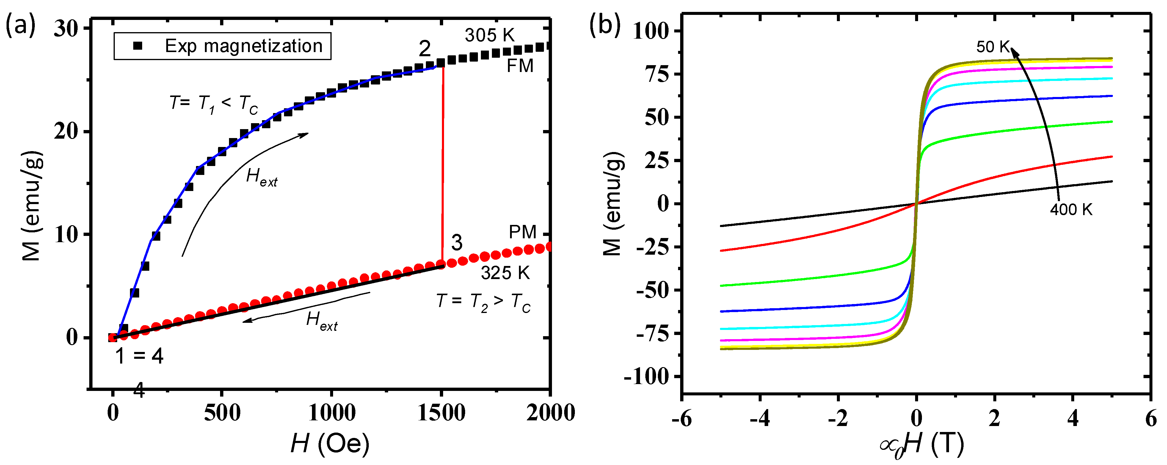
The thermomagnetic material undergoes a series of changes in its state of magnetization and temperature in the thermomagnetic cycle illustrated in
Figure 1a. The magnetic field is usually generated externally by permanent magnets. Assuming that the initial temperature state of the material is below the Curie temperature (
T1 <
TC) and it is unmagnetized (at point 1). At this point, the material is ferromagnetic, which means that it allows the magnetic field lines from the external source to pass through it relatively easily. It is then brought near to the magnetic source and becomes magnetized (at point 2). At the next step, the heat load is introduced to the thermomagnetic material, which causes its temperature to rise above the curie temperature,
T2 >
TC. At this point, the material becomes paramagnetic, which results in fewer magnetic field lines passing through it (at point 3). Thereafter, the external magnetic field is removed and the cooling process is started until it returns to its initial ferromagnetic state (at point 4), where the cycle can be repeated again.
It is necessary to quantify the magnetic energy conversion and to evaluate the conversion efficiency in order to select the appropriate thermomagnetic material for heat harvesting application. The maximum magnetic energy conversion that happens in a material during magnetization and demagnetization is obtained from the area enclosed by the M–H curve (as illustrated in
Figure 1a). The area can be expressed mathematically as:
The magnetic energy converted in each cycle is equivalent to the net work done by the material. The total heat gained by the material is equivalent to the sensible heat gain due to temperature changes as well as any entropy generated by the expression in (2). The isothermal heat addition due to entropy is ignored in this case as it is much lower compared to the sensible heat addition in a heat harvesting application [
3].
The efficiency of the thermodynamic cycle is measured by the ratio of the work done to the total heat addition per unit volume of the material as defined in (3).
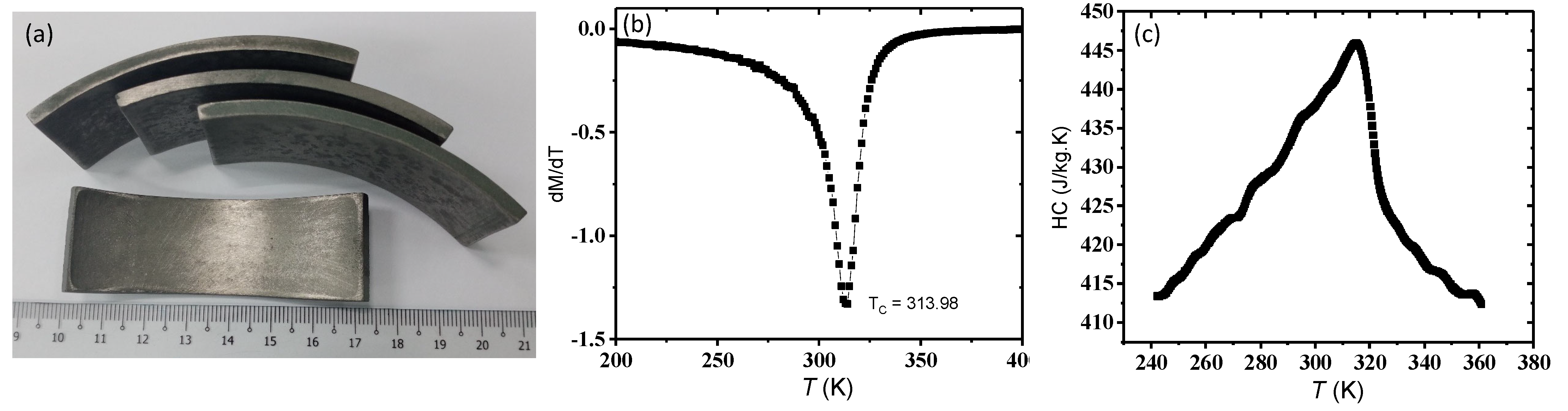
The thermomagnetic material is processed by the powder metallurgy method. The process starts with ball milling of the powder of the raw materials mixed according to the final composition of the thermomagnetic material that is desired. This is then followed by the compaction of the finely mixed powders under high pressure. Finally, the compacted part goes through a heat treatment via a sintering process. Thermomagnetic material with the following composition, Mn
2Fe
1Sn, has been synthesized and produced to the desired shape and size (
Figure 2). The final part that is produced has a density of approximately
. Samples of the material are characterized using the physical property measurement system (PPMS) and vibrating sample magnetometer (VSM) instrument to determine its temperature dependent magnetic properties.
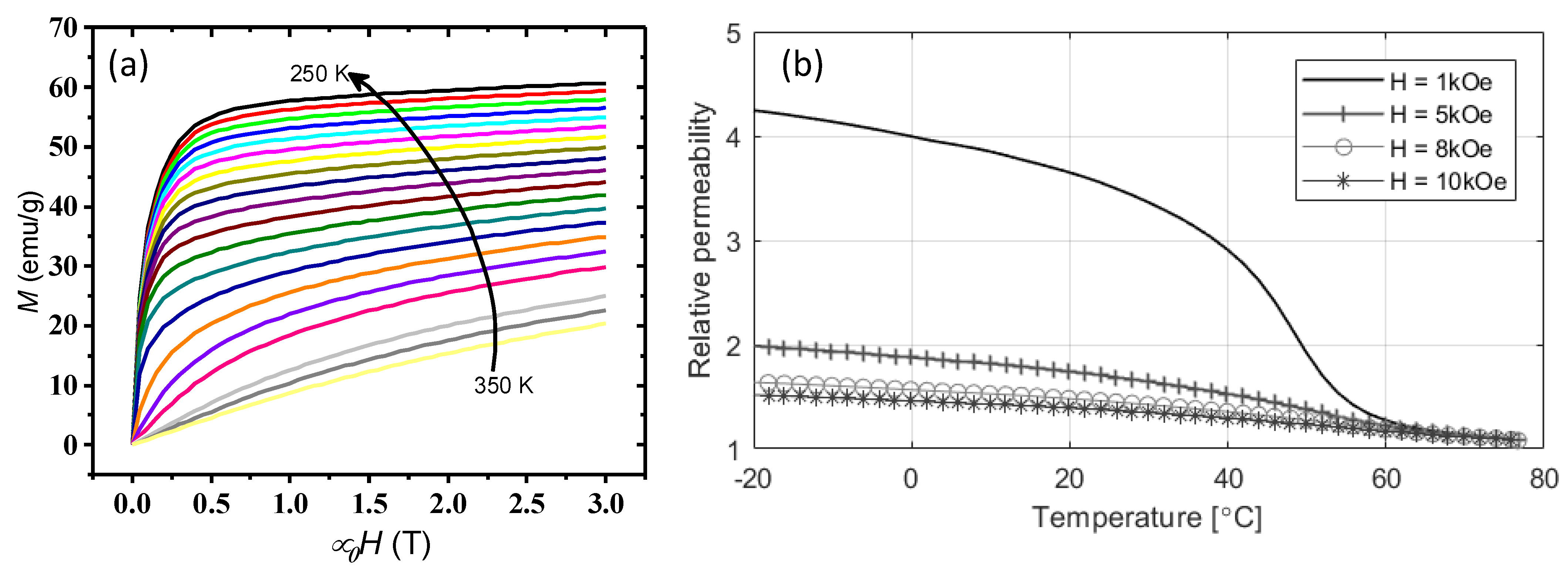
Figure 1b shows the M–H curve for the thermomagnetic material at different temperatures obtained through the PPMS. From this set of measurement data, it is possible to work out the thermomagnetic material energy conversion efficiency as defined by (3).
Firstly, it is necessary to identify the four operating points from this set of data that describes the thermodynamic cycle illustrated earlier in
Figure 1a. The curie temperature of this composition of material is approximately
based on the measurement data shown in
Figure 2b. The temperature difference between the hot and cool state is kept at
. This means that
, while
to achieve the targeted temperature fluctuation around the Curie temperature. The applied magnetic field is estimated to be approximately 1500 Oe, which is the magnetic field strength at some distance away from the permanent magnet source. Based on the above operating conditions, the magnetic energy converted in each cycle is equivalent to approximately
. On the other hand, the sensible heat addition works out to be approximately
(from
Figure 2c). This gives a cycle averaged thermal to magnetic energy conversion efficiency of approximately 2.6%. This would serve as the basis for comparison with the energy conversion efficiency that can be achieved by the rotary thermomagnetic motor, which will be discussed shortly.
4. Experimental Measurements
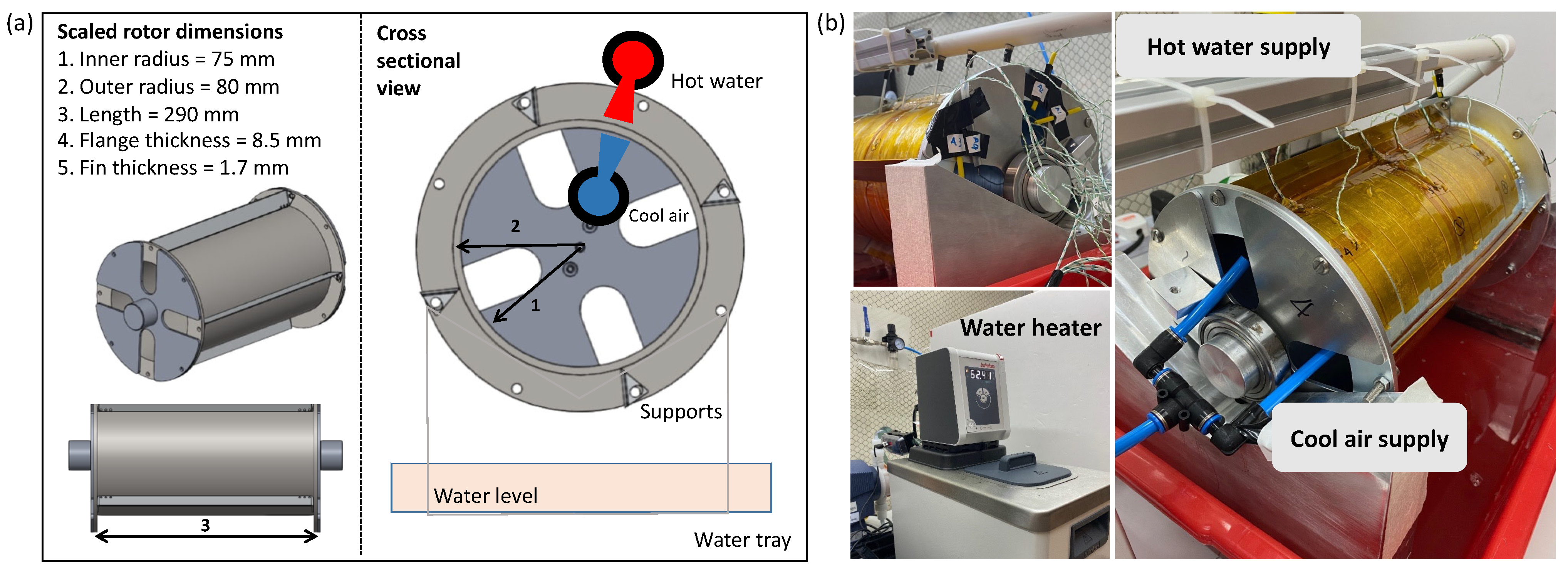
A scaled rotor assembly is constructed to collect experimental data to evaluate the heat transfer parameters described in the previous section. This scaled rotor is constructed from steel with the dimensions shown in
Figure 3. The dimensions of the scaled rotor are chosen to be between the lower and upper bounds of the design parameters that are used in the subsequent design analysis presented in
Section 5. The scaled rotor assembly is subjected to impingement heating and cooling using hot water and cool air as the heat transfer medium. Hot water is supplied from a hot water bath through a pump via a network of pipe and nozzles which directs the water to the outer surface of the rotor. Cool air is supplied by a pressurized air source through a series of piping which directs the air to the inner surface of the rotor. The hot water and cool air is supplied sequentially by alternating the output from either source via a control valve. At the same time, the rotor is locked in position throughout the experiment so only one segment of the rotor assembly is heated and then cooled sequentially.
The temperature measurement taken at several points of interest is shown in
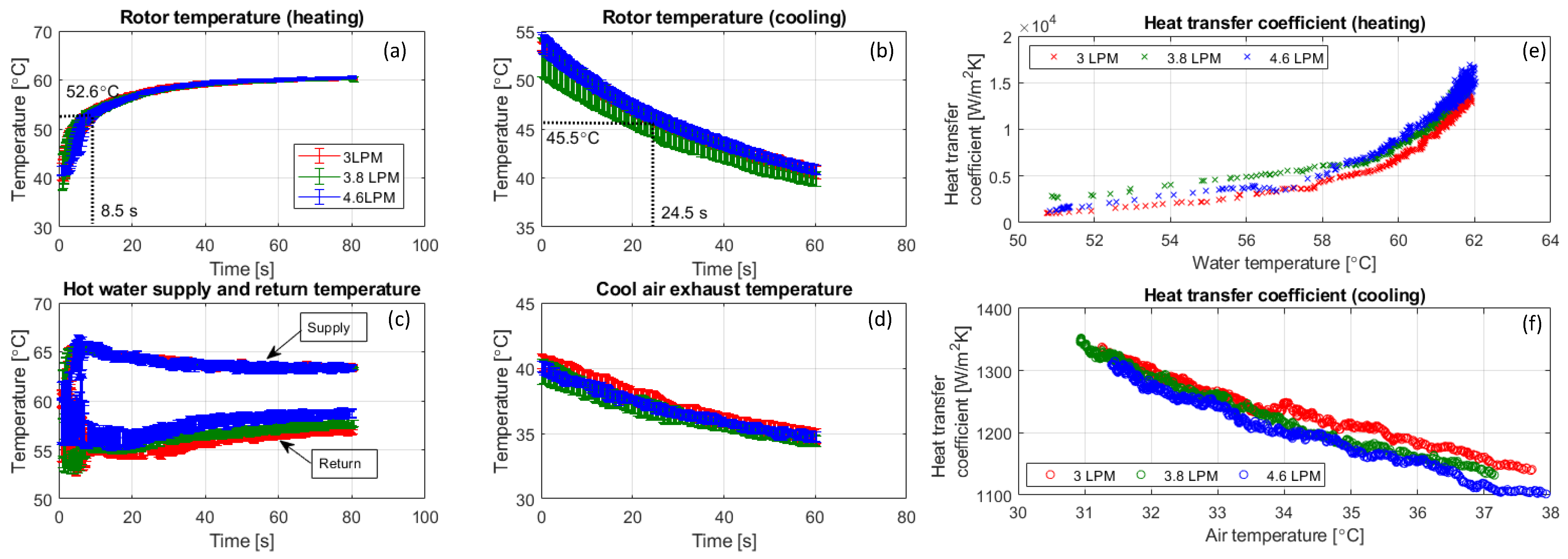
Figure 3. The rotor surface temperature measurement is taken as reference temperature of the thermomagnetic material during both heating and cooling. The data shown in
Figure 4 is a collection of several runs of the experiments that was conducted to obtain the average temperature. The line plot gives the mean value of the several data points collected, while the error bar shows variation of the data within one standard deviation. The different colored plots correspond to the temperature data collected at various flow rates of the hot water supplied. The cool air supply is kept constant at a regulated pressure of approximately 1.5 bar, which gives rise to an overall air flow rate of approximately 0.05 m
3/s or around 106 CFM. The equivalent heat transfer coefficient is evaluated using (19) and (20), with the results shown in
Figure 4.
The plot shows that the heat transfer coefficient during heating varies between 1200 to 16,000 W/m
2K, while it ranges from 1100 to 1350 W/m
2K during cooling. It is expected that the heat transfer increases with the rate of hot water supplied as indicated by upward shifted plots in
Figure 4. The heat transfer during cooling remains relatively constant as air supply is kept at the same level across the several experiments. The averaged heat transfer coefficient during heating is approximately
, while it is approximately
during cooling. The data presented here shows that there is variation in the heat transfer parameters with the operating conditions, such as the temperature of the object and fluid [
26,
27]. The data obtained from this experimental investigation provides an estimate of the upper and lower bounds of the heat transfer coefficient that will be considered in the subsequent design analysis.
5. Design Analysis and Optimization
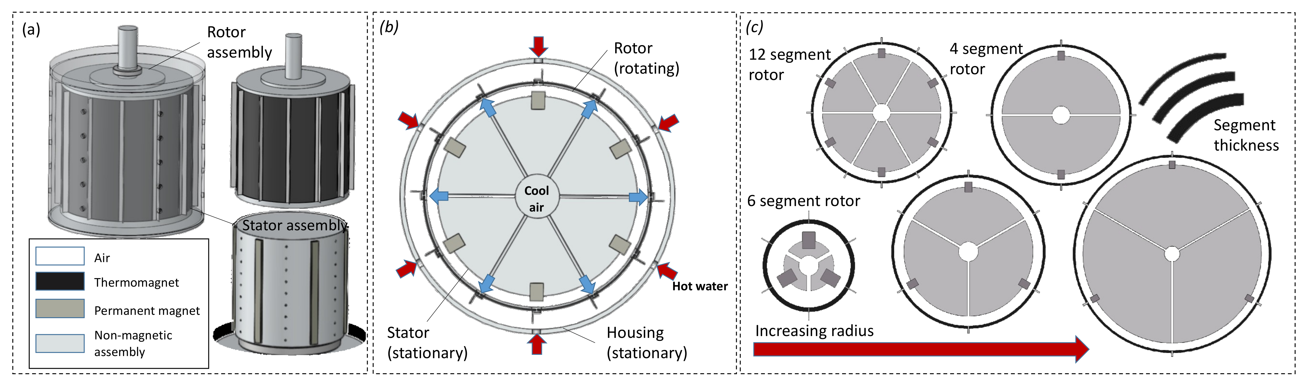
The rotary thermomagnetic motor presented in this paper consists of a rotor and a stator, as shown in
Figure 5a. In this design, the thermomagnets are introduced to the rotor, which is divided into an even number of segments, while the permanent magnets are housed in an internal stator assembly. These thermomagnets are separated physically and thermally insulated from each other by spacers found on the rotor body. Alternate segments of the thermomagnets are heated and cooled in the hot and cool zones, as shown in
Figure 5b. In the hot zone, hot water is supplied to the outer rotor surface through a series of nozzles in the housing, and the water is then directed toward the outer periphery of the rotor by the spacers. In the cool zone, the cool air is directed towards the inner surface of the rotor through internal channels in the stator. As the rotor rotates, each thermomagnet segment will go through the hot and cool zones sequentially.
The dimensions of the rotor will be one of the key design considerations along with the number of rotor segments. In addition, operating conditions, such as the temperature of the heat source, the rate of heating, and cooling, will also be considered in the subsequent design analysis. The list of design variables are given in
Table 1, with the associate range of values to provide some constraints over the design space. There is a periodicity that is observed in the rotor assembly, which is illustrated in the insert of
Figure 5c. One period of rotation is equivalent to the arc angle covered by two segments of the rotor. For example, a 12-segment rotor would have a periodicity that is equivalent to 60°, while a 6-segment rotor would have a periodicity of 120° and so on. This makes it possible to analyze rotor configurations with a different number of segments. It should be pointed out that the alternating heating and cooling arrangement remains unchanged even though the number of segments may vary.
The rotor is driven by the torque generated due to changes in reluctance of the thermomagnetic material, as described in
Section 3.1. The reluctance torque that is generated on the rotor is described by (9), which is a function of the magnetic flux density on the rotor surface. The flux that is generated is in turn dependent on the permeability of the material as well as its position relative to the permanent magnet. It should be noted that the reluctance torque is position dependent. The rotor dynamics is described by the following equation:
where
is the inertia of the rotating mass and viscous friction is expressed as a function of the rotation speed
and friction coefficient
. The rotor speed is determined by solving (21) and the rotor position is evaluated through the time integration of the speed over time.
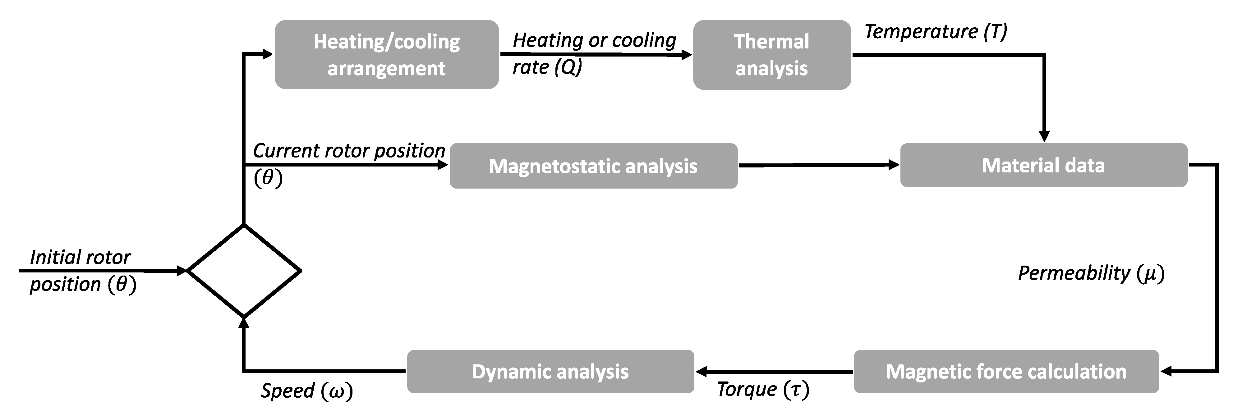
The position of the thermomagnet relative to the permanent magnet and the strength of the magnetic field as well the temperature all has a significant effect on the torque produced by the thermomagnetic motor. The design process can be divided into several steps using the various models presented, as illustrated in the flowchart in
Figure 6. Firstly, the rate of heating or cooling of the material is determined by the position of the thermomagnet relative to the heating or cooling zone. Next, the temperature of the thermomagnet is then estimated using (18). Besides the temperature, the permeability of the material is also affected by the magnetic field intensity, which is also dependent on the position of the thermomagnet. The final magnetic field distribution in and around the thermomagnet is evaluated from the magnetostatic analysis described in
Section 3.1. Finally, the magnetic force acting on the thermomagnet is then evaluated using (12).
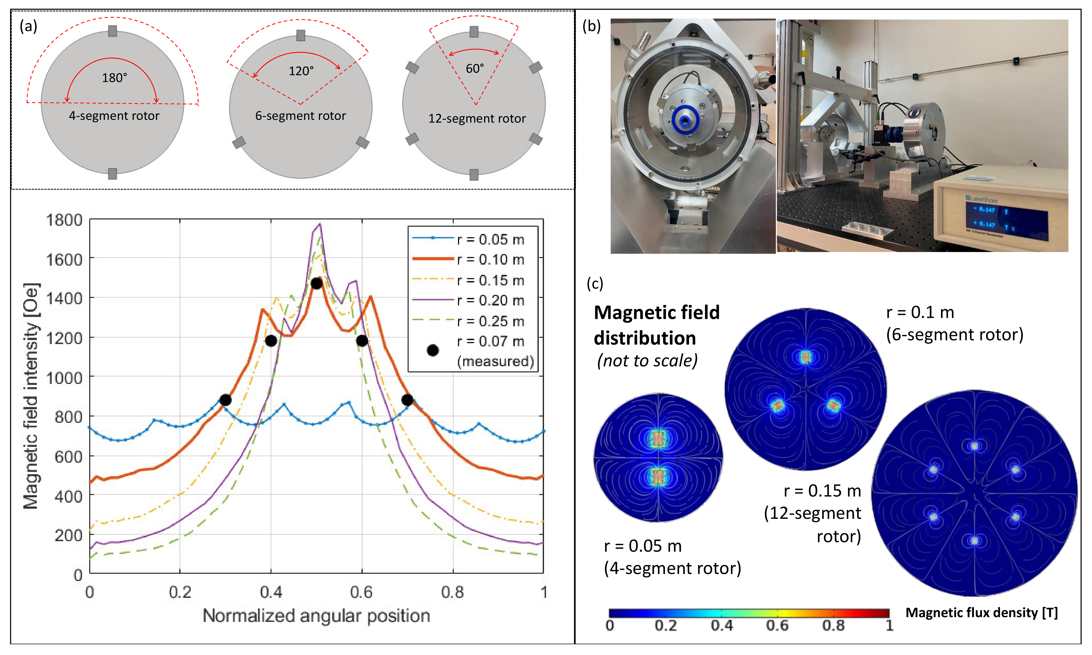
Figure 7a shows the magnetic field intensity produced by the permanent magnets at a different angular position at a radial distance of 10 mm away from the top surface of the magnet. The different colored plots correspond to the various configuration of the rotary magnetic assembly that is considered in this design analysis. Additionally, several measurement data points are plotted against data obtained from the mathematical model for comparison. The measurement is taken from an experimental set-up shown in
Figure 7b using the Lakeshore 460 Gauss meter. The permanent magnet assembly shown goes with a six-segment rotor that has an effective radius of 0.07 m. There is good agreement between the measurement and the model predictions at the point of interest. It is expected that the magnetic field intensity decreases with distance from the permanent magnet. The rotor is positioned at an offset distance of approximately 10 mm away from the top surface of the magnet. This would ensure that the magnetic field intensity experienced by the thermomagnets will be within the range of values that is measured and shown here in
Figure 7c.
The permeability of the thermomagnetic material is evaluated from the magnetization data shown here in
Figure 8a, which is obtained from the material characterization procedure presented earlier in
Section 2. The permeability data presented here is converted into a look-up-table with the temperature and magnetic field intensity as inputs. With the material properties fully defined, the torque that is produced by the device as well as the rotor speed can be estimated using (21). Finally, we can work out the position of the rotor in time through the time integration of the instantaneous rotor speed. This analysis is performed at each instance of time to obtain the time evolution of the rotor speed and torque generated. The interdependence between the various variables that links the different physical processes that happens in the device makes the design analysis non-trivial. The results obtained from this analysis will be presented in the following section.
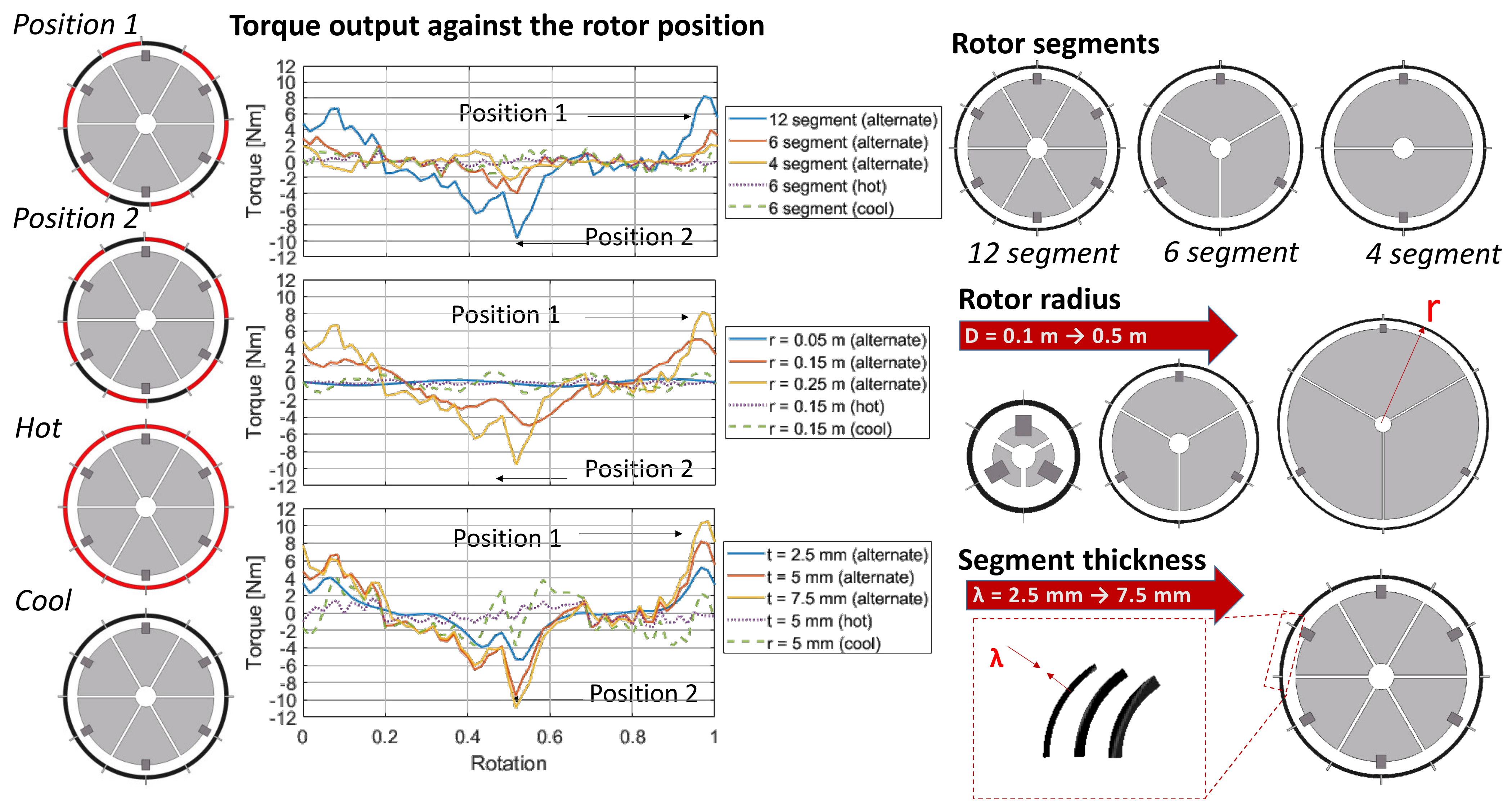
Figure 9 shows the plot of the torque that is generated as a function of the rotor position with rotor as well as the temperature state of the thermomagnet. It is clear from the data that there is a range of rotor positions that produces a positive torque (counter clockwise). The maximum positive torque occurs at a rotor position that corresponds to approximately 95% of one period of rotation. The output torque level diminishes after 25% of the rotation period is completed and turns negative reaching a minimum value when approximately 52% of the rotation period is attained. The output then turns positive and reaches the maximum value again when almost one period of rotation is completed. The simulation result shows that the torque output is increased when alternate segments are either hot or cool. The torque produced is maximized when the hot segment enters the magnetic zone (position 1). On the other hand, a large negative torque is produced when the hot segment leaves the magnetic zone (position 2).
The simulation data shows that an alternating hot and cool segment is required to produce the positive torque. This leads to an alternating heating and cooling zone arrangement relative to the permanent magnets that are shown earlier in
Figure 5. The simulation data also shows that the peak torque tends to increase with the number of rotor segments as shown by the increase peak value in
Figure 9. This is also true when the rotor radius is increased as shown by the plots in
Figure 9. Lastly, the peak torque is also amplified when the thickness of the segment is thickened. This data yields important insights into the key characteristics of the rotor design that leads to greater torque output. However, the eventual torque that is produced by the thermomagnetic motor still depends on the temperature that can be attained under dynamic conditions. It should be pointed out that the segments will be in motion once the torque is produced and this rotation does have an effect on the amount of heating or cooling experienced by each segment of thermomagnetic material. This coupled thermal-magnetic effect on the rotor dynamics will be presented in the Results section.
Design Optimization
An optimization problem is defined to determine the optimal design of the thermomagnetic motor that maximizes output parameters, such as its power output
, power density
, and efficiency
. The optimization problem is typically expressed mathematically as an objective function
in the following form:
whereby
is the set of design variables given by
and
is the solution of this minimization problem. Maximum value problems are converted to a minimization problem by substituting the objective function with its negative such that
. The list of design variables considered in this optimization problem are listed earlier in
Table 1. There will be some restrictions to the physical design and these are expressed mathematically as constraints. The constraint usually applies on the design variables, such as a limit on the minimum or maximum value that a design variable can carry. Moreover, some design variables only take discrete values and additional constraints can be defined to cater for such discrete variables.
Gradient based optimization methods require the evaluation of the objective function and its derivative at various points in the solution space. If the necessary conditions are not met, then the solution is advanced to the next feasible solution by a step change in given by . Linear or quadratic approximations of the function is typically used in place of the actual objective function during the optimization process. The method progresses in a step wise fashion to search for the optimal solution. Firstly, a direction of search is determined, then the step size is selected with the aim of minimizing the objective function at each iteration. There are various methods used to decide on the search direction and step size. The following description provides details of the key steps involved in a Quadratic Programming (QP) method.
For a constrained optimization problem, the objective function is first replaced by a Lagrange function, which is defined as such:
where
is the objective function and
is the
ith constraint out of a total of
constraints while
is the associated Lagrange multiplier. The following quadratic approximation of the Lagrange function is used to determine the search direction,
where
is the gradient of the objective function and
is the Hessian matrix. The search direction is determined by solving (25), which is derived from the necessary conditions for a minimum solution of (24)
where
is the gradient of the
ith constraint function such that
and
, while
is the Lagrange multiplier first defined in (23) expressed in vector form.
Iterative numerical methods are typically employed to solve such constrained optimization problems. Approximations of the objective and constraint functions (or Lagrange function) as well as its derivatives are evaluated at each iteration. The solution is then moved from one point of the solution space to the next based on the search direction that minimizes the objective function and its derivative. This continues until a termination criteria is met, which is often when the optimal conditions are met or when there is no further noticeable change in the objective function value. The calculations performed in each iteration of the algorithm are listed here:
- 1.
Obtain initial estimate of the design variable and set the Hessian matrix . Initialize the penalty parameter , permissible constraint violation and convergence parameter ;
- 2.
Evaluate the constraint functions and determine the maximum constraint violation, which is defined as ;
- 3.
Determine the search direction
and Lagrange multipliers by solving (25);
- 4.
Stop if the termination criteria is met and the maximum constraint violation is otherwise continue;
- 5.
Evaluate the sum of the Lagrange multiplier defined as
and set the penalty factor ;
- 6.
Update the design variable where is defined as the step size determined from a line search method;
- 7.
Update the penalty parameter ;
- 8.
Update the Hessian matrix using (26)–(32) and increase the counter , then return to step 2.
The gradient of the Lagrange function is used to estimate the Hessian matrix in a constrained optimization problem based on the quasi-Newton Hessian approximation method proposed by Broyden–Fletcher–Goldfarb–Shanno (BFGS) [
28]. Correction factors are introduced to the Lagrange function in the BFGS method to ensure that the Hessian matrix is definitively positive. Furthermore, additional variables are introduced in the intermediate steps before a final estimate of the Hessian matrix can be obtained. The approximation method first starts with the definition of the step change given here:
where the working variables
,
, and
are defined by (24), (25), and (26), respectively.
is determined from the following cases
where
and
are defined in (28)
Finally, the Hessian matrix is updated according to (32)
where
The sequential quadratic programming (SQP) method described here is the preferred numerical method in many commercial software packages, such as Matlab, because it is stable, accurate, and efficient to compute. In the subsequent design optimization, the ‘fmincon’ solver available in the Optimization Toolbox of Matlab using the SQP algorithm is deployed during the optimization process.
6. Results and Discussion
Figure 10 shows the output characteristics of the thermomagnetic motor with nominal parameters. The torque produced by the motor climbs to a final maximum value of 0.9 Nm after approximately 40 s, which it maintains for the remaining duration of the simulation. The motor finally settles at a rotation speed of approximately 17 RPM which gives an averaged power output of approximately 1.7 W. While the torque and speed settle at a more or less steady value, the temperature is seen to be oscillating below and above 75 °C. This fluctuation is required for a continuous positive torque to be produced, as discussed earlier in
Section 5. However, the temperature variation happens at an elevated temperature beyond the Curie temperature of the material. This shows that the device is not yet running optimally.
Figure 10c shows the heat flow in and out of the material evaluated using (17). There is a huge flow of heat into the material at the start in order to heat up the material from the ambient temperature. Thereafter, the rate of heat flow reduces to an average value of 23 kW when only the inflow of heat is considered.
Based on the data generated from the model, the power output and efficiency of the thermomagnetic motor with the nominal parameters is fairly low and quite insignificant. This is because the nominal parameters are selected to maximize the inputs to the device as well as the amount of thermomagnetic material used. However, this does not necessarily yield the most output from the device since the operating conditions should be selected to match the design of the thermomagnetic motor. For instance, using more thermomagnetic material would mean more heat is required to power the device which could lead to a lower overall efficiency. On the other hand, using too little material would mean less reluctance torque generated leading to lower outputs. These interactions will be analyzed further in the subsequent design analysis which shows how the output characteristics of the device can be further improved through careful selection of the design and operating parameters.
The output torque generated by the thermomagnetic motor and the power output are critical measures of performance. In addition, the power density and efficiency of the thermomagnetic motor provides a useful measure of the output against the amount of material used as well as the amount of heat energy required. These measures form the basis of comparison with other similar heat energy harvesting devices. The instantaneous torque and speed are derived from (21), while the instantaneous power is given by the following expression:
The time averaged values of the various output parameters (collectively referred as
) are evaluated from the RMS value of the parameters using the expression given in (34).
where
is the time duration of the analysis, which is chosen to be 300 s. The efficiency of the thermomagnetic motor is defined as the percentage ratio of the time averaged power output
to the averaged heat supplied
such that:
Finally, the power density
is given by the expression in (36) where
is the volume of the thermomagnetic material used.
The subsequent design analysis is performed in a step wise fashion in which only the parameters of interest are varied at each step of the analysis, while the other parameters are kept constant based on the nominal values given in
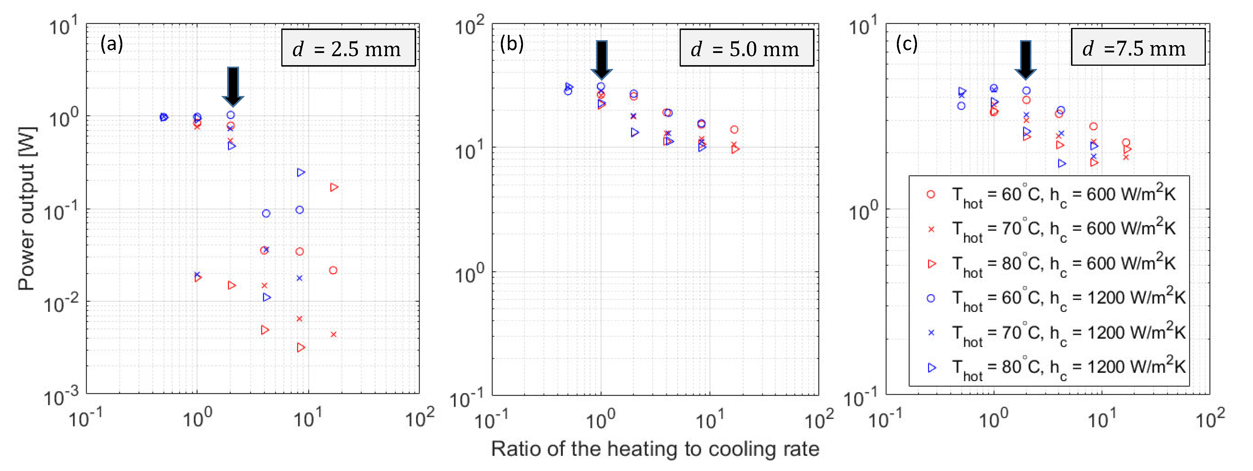
Table 1. The average power produced by the thermomagnetic motor with nominal design parameters is plotted against the ratio of the heating to cooling rate as shown in
Figure 11. The colored plots correspond to a higher or lower rate of cooling, while the different markers correspond to the various temperatures at which the hot water is supplied to the device. The sub-plots in
Figure 11 show the variation in the power generated by devices with varying thickness of thermomagnetic material used. Generally, the power output is enhanced at a higher rate of cooling, i.e., when
. In addition, the data shows that the power generated tends to peak when the rate of heating is equivalent to the rate of cooling (at points where x-axis is equal to 1). There are some instances where a lower heating rate is beneficial, such as when thicker thermomagnetic material is used. The temperature of the hot water supply does not appear to have a significant effect on the output of the device. On the other hand, the thickness of the material has a significant effect on the power output. There is almost an output increase of 10 times when the thickness of the material is increased from 2.5 mm to 5 mm. However, any further increase in the thermomagnetic material thickness does not yield any more gains in the output.
The thermal boundary conditions that are necessary for the thermomagnetic motor to generate a higher power output is shown (by the black arrow) in
Figure 11. These conditions are used in the subsequent design analysis. The sub-plots in
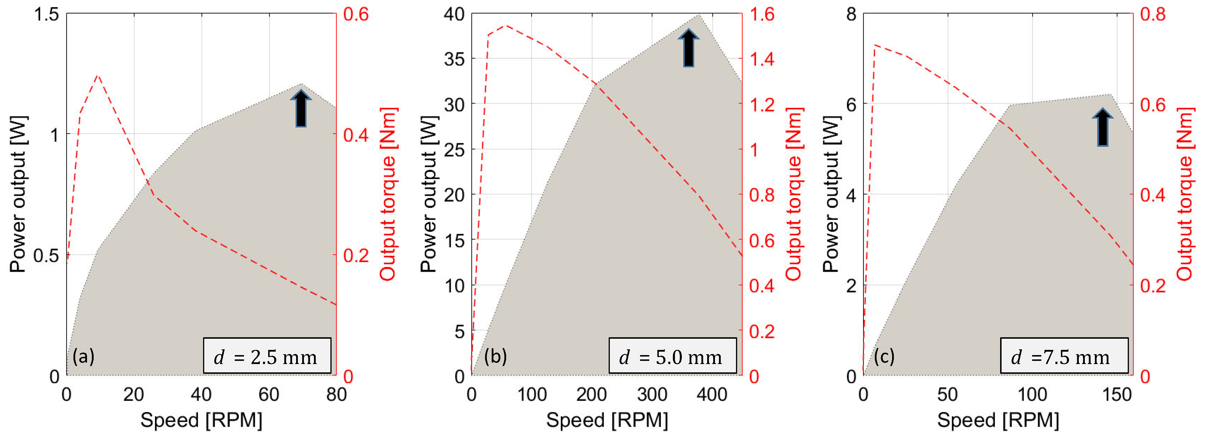
Figure 12 show the power (shaded) and torque (line) generated by the thermomagnetic motor with different thicknesses of the material used. This set of data is generated assuming that the rate of heating and cooling are closely matched according to the ‘ideal’ conditions described earlier. The data shows that there is an optimal speed at which power transfer and the corresponding output torque level are maximized. Therefore, it is important to carefully select the braking torque applied by the load onto the device to ensure that the thermomagnetic motor will operate at a speed that maximizes the power transfer. The point where power transfer is maximized is highlighted (by the black arrow) in
Figure 12 and the torque applied onto the load is kept constant in the subsequent analysis.
The power density is first defined in (36) and it is plotted here in
Figure 13 against the aspect ratio of the thermomagnetic motor. The aspect ratio refers to the ratio of the external length to the diameter of the rotor. The different colored plots refer to data generated from rotors with a varying number of segments, while markers are used to differentiate rotors of different diameters. The data generated from devices with varying thickness of thermomagnetic material is shown in the sub-plots in
Figure 13. The data shows that the power density tends to peak at aspect ratios between 1–2. This trend is observed with rotors of different diameters, but it is most pronounced for rotors with larger diameters. From this set of data, it is observed that the higher power density can be generated from a 12-segment rotor. However, when thicker thermomagnetic material is used, higher power density is achieved with a smaller number of rotor segments instead. Nevertheless, the highest power density recorded is still from a 12-segment rotor with a diameter of 0.4 m and a length of 0.5 m.
The design analysis shows that the power density tends to increase with the number of segments as shown by the data provided in
Figure 13. This is expected since having more segments increases the useful area of the rotor, where heat can be introduced. This also means that there is more effective use of the thermomagnetic material to produce the torque for a rotor of a particular radius. However, there is a practical limit of the number of segments of thermomagnetic material that can be fit into a rotor. In addition, increasing the number of segments would mean that there is less time for the material to be heated up and cooled down at a given rotational speed. With the limits of heat transfer to and from the fluid, the speed of rotation has to be reduced correspondingly when there are more segments of material used. Therefore, the net effect of increasing the number of segments on the power output is not always positive since the power output is a product of both the torque and the speed.
The design analysis presented earlier shows that the thermomagnetic motor output is sensitive to the following parameters: (i) ratio of the heating and cooling rate, (ii) aspect ratio of the rotor, (iii) number of rotor segments, and (iv) thickness of thermomagnetic material. The preceding discussion shows how the output changes against selected parameters, while the other parameters are kept constant. It can be expected that there are further interactions between these parameters, and it is possible that there is a set of parameters that yields the ‘optimal’ output. A design optimization is performed based on the optimization method presented earlier in
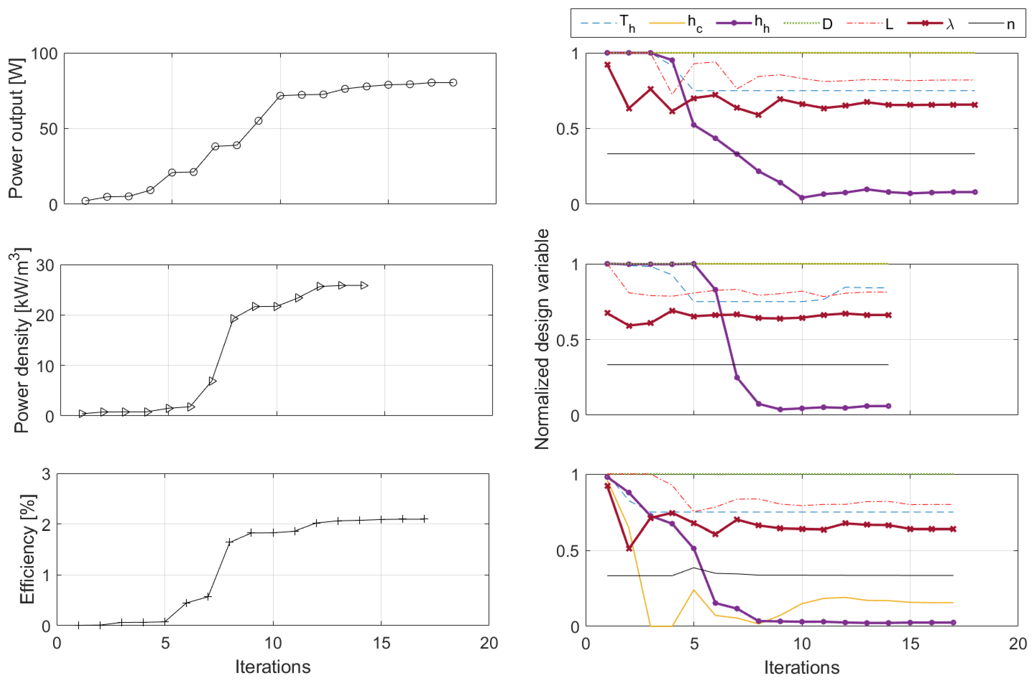
Section 5. The objective of this design optimization is to maximize each of the following output parameters: (a) power output, (b) power density, and (c) efficiency of the device. Three separate runs of the optimization routine were performed with the data generated in each run plotted in the sub-plots in
Figure 14.
The design variables are normalized before they are plotted on the same scale in
Figure 14. There is significant variation in the variables as the optimization progresses. The largest change is observed in the heating rate
as well as the thickness
of the thermomagnetic material. This is indicative of the high sensitivity of the output to these variables. The data also shows an increasing objective function value as the optimization progress, which implies that the quadratic programming method implemented here in this study is able to move the solution toward the optimal. However, further fine tuning of optimization parameters or algorithm is not considered. The results obtained from the design optimization are shown in
Table 2, with the corresponding set of parameters that maximizes each of the targeted output.
There is a slight variation in the operating parameters of the thermomagnetic motor depending on the desired output characteristics. For instance, the rate of cooling and heating is maintained lower in order to maximize the efficiency of the device. On the other hand, a higher rate of heating and cooling is required to maximize both the power and the power density. It is also not necessary to increase the heat source temperature beyond the 60 °C in all instances. The result from the design optimization also shows that there is an ‘optimal’ set of design parameters that give the most desirable output characteristics. A 12-segment rotor that is 0.5 m long with a diameter of 0.4 m using thermomagnetic material with a thickness of 5 mm is the design configuration that leads to the most favorable outcome for all 3 of the output measures considered.
The design analysis and optimization show that the thickness of the thermomagnetic material has a significant effect on the output characteristics of the thermomagnetic motor. Thicker material tends to increase the production of the reluctance torque but it also requires more heat and time to bring about a change in temperature which indirectly reduces the output over time. These counteracting factors therefore lead to an ‘optimal’ thickness of the material that yields larger outputs. It is also observed that a larger rotor diameter and longer rotor yields higher power outputs. This is expected since the reluctance torque produced is proportional to the length and diameter based on (12). However, the maximum power output is obtained not from the largest diameter but at an intermediate diameter instead. This indicates again there are conflicting factors that lead to an ‘optimal’ diameter. Additionally, increasing the length of the rotor with a particular diameter increases the power density but only up to a point where it starts to level off. This shows that the power output of the device will scale proportionately with the rotor dimensions but any further increase does not yield significant gains in output per unit of additional thermomagnetic material used.
7. Conclusions
A rotary thermomagnetic motor using a soft magnetic material (Mn2FeSn) with a low Curie temperature that is suited for heat energy harvesting is introduced in this paper. A design analysis and optimization of this thermomagnetic motor is presented. A mathematical model coupling the heat transfer, magnetic interactions, and rotor dynamics in the thermomagnetic motor is developed in this work. Measurement data obtained from the material characterization, scaled rotor, and permanent magnet assembly provide reference input values to the model. The multi-physics model is used to make predictions of the power output, power density, and efficiency of the motor against the various design and operating parameters. From the design analysis, it is determined that the thickness of the thermomagnetic material has the most significant effect on the output characteristics. Thicker material tends to increase the torque production but it also requires more heat and time to bring about a change in temperature, which indirectly reduces the output over time.
Increasing the number of segments, length, and diameter of the rotor increases the power output. At the same time, the power density is also increased but only up to a point beyond which it does not yield any significant gains in output per unit volume of additional thermomagnetic material used. The result from the design optimization also shows that there is an ‘optimal’ design configuration that results in the largest power output, power density, and efficiency. It is also observed that a higher rate of cooling leads to more output, especially when this is matched to a similar rate of heat supplied to the thermomagnetic motor. The data shows that there is an optimal speed at which power transfer is maximized and so it is necessary to load the thermomagnetic motor appropriately in order to drive it at the desired speed. After the optimization, it is estimated that the rotary thermomagnetic motor is able to produce up to 88 W of power with a power density of approximately 27 kW/m3 of thermomagnetic material used, while a maximum thermal-to-mechanical energy conversion efficiency of 2.1% is possible. With further optimization, it is possible to determine the suitable operating parameters that achieve the right balance between the power generated and the conversion efficiency of the device to meet the requirements of the heat energy harvesting application.


