Abstract
The annual electricity trade scheduling is the basis of long-term power generation scheduling. In recent decades, the ratio of new energy generation in China has increased annually, and the electricity market has operated under the “market electricity” and “planned electricity” double track mode in recent years. However, the existing annual electricity trade scheduling methods are extensive and cannot adapt to the new situation of “market electricity” and large-scale new energy generation. The annual scheduled energy of the power units is set as a decision variable, and a novel annual energy scheduling optimization model based on Gini coefficient of fairness is presented in this paper. In this model, “market electricity” capacity is conversed monthly, considering peaking reserve demand and monthly characteristics of new energy generation. The fairness constraint set based on Gini coefficient is introduced into the optimization model to solve various fairness problems. Simulation results show that the introduction of the Gini coefficient and the optimization model considering the monthly conversion of marketing electricity capacity can obtain more accurate and reasonable electricity distribution results, and the peaking demand can be considered more fairly and effectively. The proposed method provides a feasible solution to the annual electric energy scheduling for dual-track operation country such as China.
1. Introduction
The annual electricity trade scheduling is usually considered as the basement of the formulation and implementation of the electricity trade scheduling in China. It is the most important processes of the long-term power generation scheduling. The annual electricity generation demand should be reasonably allocated to each unit according to certain principles. The average allocation method according to the generating hours of each unit is the most primitive and traditional method for annual electricity allocation in China, which ensures the “fairness” in traditional sense and is the method of electricity energy scheduling continuously adopted in China in the past years.
At the beginning of this century, “energy-saving generation scheduling” was put forward in China with increasing attention to the energy environment. Under the background of energy-saving generation dispatching, provinces generally adopt the differential electric quantity model. All fossil energy generating units were classified or graded according to the unit type, energy consumption grade, capacity difference, environmental protection level, location and other factors. Then, according to the total electric quantity and the total number of “gears” or “stages”, the difference of power generation utilization hours or basic generation utilization hours between each gear is determined [1,2,3,4]. The differences of unit power generation utilization hours further expanded between large capacity high efficiency environmental protection units and small capacity units in the literature [5]. Two kinds of annual electric energy scheduling mathematical models based on dynamic level difference are established to maximize energy conservation and emission reduction, respectively. Electricity purchase cost minimization together with energy conservation and emission reduction are taken as the optimization objectives in order to promote the realization of energy saving and emission reduction targets in the formulation of annual electricity plan. The effect of energy conservation and emission reduction was further optimized with this method. However, there is still a large space for improvement because the optimizing model is still extensive, and the calculation granularity is large. It cannot really “reduce energy consumption and pollutant emission to the maximum extent”. Moreover, the determination of the difference of generating utilization hours between units of different grades lacked necessary theoretical basis to support, so it was difficult to achieve a fairness recognized by all power plant operators.
With the gradual opening of the electricity market in China, “market electricity” has become an indispensable part of medium and long term electricity trading, which mainly deals directly with large users. The compilation process of annual contract electric energy under the impartial and open dispatching modes, namely, traditional dispatching, complete market, and limited bidding was proposed in [6]. However, specific models and methods were not researched. A two-stage dynamic programming algorithm of long-term energy scheduling modeling for the power systems with multilevel hydro and thermal power units was proposed in [7]. A hybrid Dantz–Wolf decomposition and subgradient algorithm for long term power generation planning is proposed in [8]. In paper [9], an annual optimal scheduling model is proposed to reduce investment costs and improve energy saving and emission reduction effects. However, the formulation method and model of annual electricity scheduling were not involved in the above studies. In addition, there are obvious differences between foreign power market system and the electricity system with planned electricity in China.
Under the electric power system and mechanism in China, some important public electricity and some service electricity need to be guaranteed. Therefore, the Ministry’s distribution plan is formulated and issued by the State as planned electricity. The “dual track” operation of planned electricity and market electricity will coexist for a long time in China [10,11,12]. However, the existing research results have not been reported on the “dual track” operation mode for the annual electricity trading scheduling model. At the same time, with the proportion of new energy generation such as wind power and photovoltaic increasing year by year, it brings more pressure to the system adjustment because the output of new energy is also more seasonal. The specific implementation of each month has not been taken into account in existing methods of electricity energy scheduling. The implementation pressure and deviation of electricity energy scheduling have increased year by year. They can hardly adapt to the new situation of “market electricity” and large-scale new energy generation. To sum up, the existing annual electric energy scheduling approaches are extensive and cannot adapt to the new situation of “market electricity” and large-scale new energy generation, which means a novel annual electric energy scheduling method need to be studied to deal with the new situation and to improve the modeling accuracy.
In order to make up for the shortcomings of existing methods, the formulation of annual electricity energy scheduling should be improved from the following two aspects. First, the annual electricity energy of each unit is taken as the decision variable in the optimization modeling. The accurate optimal electric quantity allocation result is obtained by solving the continuous optimization model, so as to achieve the true sense of “minimizing energy, resource consumption and pollutant emission”. Secondly, the recognized fairness index should be applied to restrain the generating hours of each unit as a whole, so as to obtain the fairly allocation scheme which could be accepted by all the power producers.
The Gini coefficient is an indicator of judging fair income distribution, presented by the famous Italian economist Gini in 1912. It can be used to measure the fairness of income and consumption of equity, allocation fairness of resources, and any other things of the distribution of equal status. It is the internationally recognized measure of things distribution fairness in recent years. It has been widely applied in economics, humanities, environmental science, power system, and other fields [13,14,15,16,17,18].
If the annual electricity energy scheduling was modeled by introducing the Gini coefficient to measure the fairness of the energy scheduled for each unit, and the annual scheduled electricity energy for each unit is directly set as the decision variables, the balance between energy saving and emission reduction can be realized.
Considering the current “market electricity” and “planned electricity” double-track operation mode and the new situation of new energy generation ratio increasing year by year, a novel annual electricity energy scheduling optimization model was presented in this paper based on the Gini coefficient fairness index. In the model, the problem of traditional annual electricity planning method being too extensive and lack of theoretical basis for fairness was solved. Through introducing the monthly electricity characteristics considering load balance constraints, based on the user load reserve demand monthly capacity conversion “market electricity” and introducing the Gini coefficient of fairness constraint set, the balance among the fairness, the energy saving and emission reduction could be achieved within acceptable range of the generation producers under the double-track operation mode. The proposed method provides a feasible solution to the annual electric energy scheduling for dual-track operation country government, such as China.
2. Gini Coefficient Fairness Index
2.1. The Concept of Gini Coefficient
The Gini coefficient was proposed on the basis of a Lorentz curve. It is used to reflect the social statistics of income level allocation fairness. Gini coefficient is an economic statistic index reflecting fairness on the whole. The Lorentz curve is a curve that reflects the fairness of a given income allocation which is shown in Figure 1.
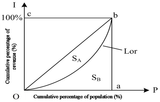
Figure 1.
Lorenz curve.
Based on the Lorentz curve, the Gini coefficient is:
The Gini coefficient is equal to twice the area value of . For convenience of calculation, it is usually converted to the area value of . According to Formula (1), when the area of is zero, the allocation is absolutely fair. The larger the partial area is, the more uneven the distribution is.
2.2. Gini Coefficient Calculation Method and the Meaning of Value Range
The calculation methods of the Gini coefficient mainly include direct calculation method, regression curve method, radix bisection method and group decomposition method [19]. According to regulations of relevant United Nations organizations, the meanings of different value ranges of the Gini coefficient are shown in Table 1. If the value of the Gini coefficient is less than 0.4, the fairness is basically achieved. If the Gini coefficient value is less than 0.3, the fairness is better.

Table 1.
The value range meaning of the Gini coefficient.
2.3. Applicability of the Gini Coefficient as Electric Energy Fairness Index
As mentioned above, the Gini coefficient is an internationally recognized indicator of economic income equity. It can be used to measure the fairness of income, consumption and resource allocation and the equal allocation of any other things [20]. Compared with the traditional standard difference index, the Gini coefficient can not only better measure the fairness of allocation of things and the system stability under different equal allocation conditions, but also the United Nations has given its index value to measure fairness. When the Gini coefficient value is between 0.3 and 0.4, the income gap is relatively fair and reasonable, which can maintain social stability [21]. In recent years, the Gini coefficient has been widely used in many fields such as economics, environmental science, plant ecology and power system. Under the current electricity market operation mode in China, the economic income of generator sets mainly comes from electricity income. Therefore, the fairness of electricity distribution actually represents the fairness of its economic income. As the Gini coefficient is a widely accepted indicator to measure the equity of economic income, it is suitable and easy to be accepted by all power producers as an indicator to measure the equity of unit electric energy distribution.
3. Modeling Ideas
As mentioned above, the double-track operation mode of “planned electricity” and “market electricity” will exist for a long time in my countries such as in China. The so-called “planned electricity” refers to the electricity generated, supplied and used by the relevant state organs in accordance with the corresponding policies and regulations. “Market electricity” refers to electricity generation and consumption whose price is determined through market competition. “Planned electricity” and “market electricity” dual track operation is the outcome of the current round of power system reform in China. It means that in all power generation and consumption scheduling, parts of them are determined by the government and fixed by the government, while the other scheduling is generated by market competition and settled at market prices. “Planned electricity” and “market electricity” dual track operation is one of the characteristics of electricity market operation in China, which does not exist in other countries.
Under the dual-track operation mode, generation units that participate in market transactions are called “market units”. Market units usually sign a percentage of “market power” contracts. Under current market operation mode in China, all types of units have a share of “planned power”. Therefore, the electric quantity of market unit includes “market electricity” and “planned electricity”. Units that do not participate in market transactions are called “non-market units”, and the generation capacity of such units only includes “planned electricity”. Energy composition for different type of generation units is shown in Figure 2.
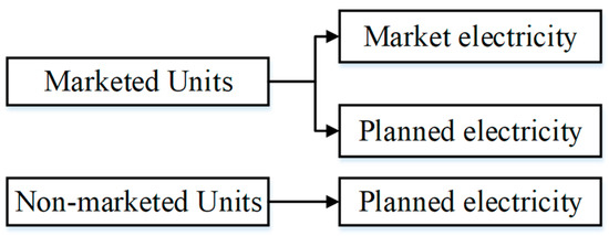
Figure 2.
Energy composition for different type of generation units in the power system in which planned and market electricity are parallel.
According to the “Opinions on the Implementation of the Plan for Orderly Release and Development of Electricity”, in principle, when arranging the planned electricity, the power generation capacity should be deducted according to the direct transaction situation. Direct transaction of large users has become an important factor to be considered in the formulation of annual electricity energy scheduling. On the one hand, the conversion of the corresponding capacity directly traded by large users involves the load characteristics of users and regions, and further involves the fairness of auxiliary services, such as peak and frequency modulation provided by each generator set, and even the feasibility of the electricity energy schedule. On the other hand, in recent years, with the increasing proportion of new energy generation integrated into the grid, such as wind power and photovoltaic, system regulation faces greater pressure [22,23,24]. Under the background of strong seasonality of new energy, the traditional electric energy scheduling method does not carefully consider the specific electric quantity implementation in each month, resulting in the increase of electric energy scheduling implementation pressure and deviation year by year. Therefore, the factors such as “market electricity” and new energy generation should be considered in the annual electricity energy scheduling model, so as to make power generation energy scheduling more refined and fair. Among them, fairness should also include the fairness of stable load rate and the fairness of encouraging “market electricity”, that is, fairness should be considered more refined. Therefore, an annual electricity energy scheduling optimization model based on the Gini coefficient fairness under the “dual track” operation mode of planned electricity and market electricity is presented in this paper. By introducing monthly electricity balance constraint, converting “market electricity” capacity by month and introducing the Gini coefficient fairness constraint set, various problems existing in current annual electricity planning can be better solved.
When the scale of direct transaction of large users increases, it is directly affected by the volume conversion of direct transaction. Since there are great differences in load characteristics, system load characteristics, and output characteristics of all kinds of new energy generation in different months, the capacity of generating units participating in large user direct transaction should be converted at least in the unit of month. However, if the capacity is converted on a weekly or daily basis, on the one hand, the calculation scale of 365 days in a year is too large; on the other hand, the consideration is too detailed, which is not good for the generation manufacturers to understand. Moreover, accurate information in daily basis is not available at the beginning of the year, so such fine granularity is practically meaningless. Therefore, in this paper, the participating trading capacity of each unit participating in direct trading is converted on a monthly basis, and the electric quantity balance model is established on a monthly basis.
For the electricity capacity conversion method, the fairness of the auxiliary services such as peaking undertaken by each unit is taken into account [25,26]. From the point of view of direct transaction, the peak load of electricity users needs the corresponding installed capacity of power generation enterprises to match. Users with high peak load occupy more installed capacity resources, so the calculation method of power users’ direct transaction capacity considering load characteristics is adopted, that is, the power generation enterprises should undertake the task of peak load regulation with direct transaction load.
In view of the fairness of scheduled electricity decomposition, the principle in this paper is to encourage power generation enterprises to participate in direct market transaction as much as possible, so the fairness constraint method of a double Gini coefficient is adopted for the generation utilization hours of planned electricity after deducting market capacity and the generation utilization hours of planned electricity without deducting market capacity. The Gini coefficient fairness constraint of planned electricity generation utilization hours after deducting market capacity can be relaxed by setting a larger Gini coefficient threshold.
4. Methodology and Mathematical Model of Annual Electricity Energy Scheduling
4.1. The Objective Function
The mathematical model in this paper aims to minimize the sum of energy consumption cost and pollutant emission cost of all units throughout the year:
where is the sum fuel consumption value of all thermal power units including the plants using gas, fuel oil and biomass and also other hydrocarbons, which is converted into standard coal.
where is the number of unit types, is the number of unit type , is the fuel consumption function of unit type , and is the annual scheduled energy of unit .
For a market-oriented generator unit, the annual total electric energy is the sum of the planned electricity energy finally distributed and the medium and long term electricity energy already signed:
where is the planned electricity energy distributed of unit, is the trading energy, and is the number of marketing unit.
For non-market generators, the annual total electric energy is the planned electric energy finally allocated:
where is the scheduled energy for unit in month .
where is the total sulfur dioxide emission, is the Coefficient of conversion of standard coal to raw coal according to average calorific value, is average sulfur content of raw coal, and is the desulfurization rate of unit .
4.2. The Constraint Conditions
In order to consider the generation characteristics of new energy and the capacity conversion of “market electricity” in a more refined way, the annual overall constraint and the monthly specific constraint are considered.
4.2.1. Annual Overall Constraints
Fairness is a very important index of annual electricity allocation under the principle of impartial and open dispatching. Compared with shorter time scale generation scheduling and economic dispatching, the annual electricity energy allocation fairness should be more strict. It should not only consider the difference of electricity energy schedule of all units within a certain fair range, but also consider the difference of electricity energy schedule of the same type of units and the same capacity units within the required fair range. The Gini coefficient is introduced in this paper as the power of all the units and various classification units set plan fairness index, the main constraint corresponding electricity power utilization hours of fairness, namely market schedule of the unit electric part of power utilization hours and non-market unit’s overall power generation using the hours of fairness, fairness constraint set power plan is established.
There are four methods to calculate the Gini coefficient value: direct method, regression curve method, radix bisection method and group decomposition method. In consideration of accuracy and operability, the direct calculation method without error factors is applied in this paper. According to the direct calculation method, the Gini coefficient is expressed as follows:
where is the mean income, is the sample size, and is the modulus of the difference between any two samples in the total sample.
Generally, the Gini coefficient is required to be less than or equal to the specified Gini coefficient threshold when it is used as a constraint condition.
where is a specified Gini coefficient threshold.
The Gini coefficient is used as the fairness evaluation index of generating hours. Therefore, the original revenue is replaced by the generation utilization hours of each unit:
Specifically, the fairness constraints considered include:
(1) Overall fairness constraint of the planned annual generation utilization hours of thermal power units:
Specifically, the fairness constraints considered include:
where is the Gini coefficient of planned generating hours of all thermal power units, is the Gini coefficient index threshold of planned generating hours of thermal power units set by the system, is the number of thermal power units, and and are the generation hours of annual planned electricity energy of unit and unit respectively, and is the average annual generating hours for all thermal power units.
where the power generation utilization hours of part of planned electricity of market-oriented units are equal to the sum of the planned power generation utilization hours of each month:
where is the generation hour of planned electricity for unit in month :
(2) Fairness constraints on annual generation utilization hours of the same type of units:
where , is the Gini coefficient of planned generating hour of type , is the Gini coefficient index value of planned generating hours of the same type unit set by the system, and is the generation hour of planned electricity for unit type k.
(3) Fairness constraints on annual generation utilization hours of units with the same capacity range:
where , is the number of unit capacity zones, is the total number of units in the capacity zone , is the Gini coefficient of annual planned electric energy of units in the capacity zone , is the Gini coefficient index of annual planned electricity of units in the same capacity partition, and is the average annual generation utilization hours of planned electricity of units in the capacity zone :
(4) Fairness constraint of planned electricity generation utilization hours after deducting market capacity:
where, is the Gini coefficient of power utilization hours of each generator set after deducting market capacity, is the generating utilization hours of each generating set after deducting the market capacity of generating set , is the Gini coefficient threshold. When setting the actual Gini coefficient threshold, can be set to a larger value to encourage generating units to participate in market transactions.
The market capacity deducted by the market unit shall be considered as the average of the market capacity converted into each month.
Among the above four constraints in the Gini Coefficient fairness constraint set, the overall fairness constraint for all units is mandatory. The fairness constraint for units of the same type and of the same capacity partition is optional. In general, the Gini coefficient of the same type or capacity partitioned units is set at a lower value than the overall Gini coefficient, i.e., its fairness requirement is higher than the overall fairness requirement. In practice, the fairness constraint can be increased or decreased for each classification of units as needed.
4.2.2. Monthly Constraints
(1) Electricity balance constraint
where, is the total electricity demand of the system in month , , , and are the forecast month for wind, hydro, nuclear and other types of power generation according to the operating arrangements.
(2) Market-based unit capacity commutation constraint
where, is the converted market electricity capacity of marketed unit in month , is the maximum load in month of directly traded user of market-based unit , is the number of users who carry out direct transactions with market-based unit , is the matching factor between the maximum load of the directly traded user of the marketed unit and the maximum load of the system, and is the adjustment factor to reflect the electricity consumption characteristics of the power system and the need for peaking reserve. Usually, the setting is the same for all direct transaction users. is the market participation incentive factor, which takes a value of 1 to indicate neither encouragement nor opposition, while a value greater than 1 indicates a higher degree of encouragement to participate in the market.
(3) Marketed unit market capacity in relation to planned capacity constraints
where, is the planned electrical generation capacity of unit in month .
(4) Constraints on the relationship between market-based unit plans and market power
where, is the planned electricity consumption of unit in month , is the amount of electricity traded directly by unit in month .
(5) Market-based unit market power balance constraints
where, is the annual direct trading of electricity between unit and customer .
(6) Constraints on the relationship between electricity generation and hours of use
where, is the number of hours of market electricity generation utilized by marketed unit in month .
When all market power is not liberalized, i.e., under the planned power system, it is unnecessary to distinguish between market and non-market units. Moreover, it is unnecessary to distinguish between market and planned power components. Fairness constraint concentration does not need to consider constraint (4), that is, the fairness constraint of planned electricity generation utilization hours after deducting market electricity capacity, and the rest is not different from the mathematical model under “planned electricity” and “market electricity” dual track operation.
4.3. Model Solving Methods
This chapter models a non-linear programming problem with only finite non-linear constraints due to the addition of the Gini coefficient non-linear constraint on the fairness of the electricity schedule. The nonlinear constraint is a nonlinear constraint with absolute values, and can be solved directly with branch-and-bound and Lagrangian dual methods. In recent years, commercial optimization software, such as IBM’s CPLEX optimization package, has been widely used to solve various linear and nonlinear programming problems in an efficient and simple manner.
5. Case Studies
5.1. System Description
A system with 20 thermal power units is used as an example for the simulation analysis. The parameters are derived from the actual operating data of a provincial network, with necessary modifications. The parameters of each unit are shown in Table A1 in the Appendix A.
According to the compilation principle, the sulfur content is assumed to be 2%, the total annual electricity demand of thermal power units is 14,950 GWh, the standard coal to raw coal factor is 1.4017, and the average sulfur content of raw coal is 0.02. Considering the fairness constraint of annual power generation utilization hours of units in the same capacity range, the capacity range of units is divided into three bands: 0–100 MW, 101–200 MW, and 201–500 MW. The capacity range is divided into three zones: 0–100 MW, 101–200 MW, and 201–500 MW.
5.2. Analysis of Calculation Results in Fully Scheduled Electricity Mode
Assuming that all units do not participate in market trading under the full planed electricity mode, two sets of fairness calculation scenarios are considered and simulated: (1) the overall Gini coefficient, the Gini coefficient of the same type of unit, and the Gini coefficient of the same capacity range unit are all taken as 0.45; and (2) the overall Gini coefficient is taken as 0.3, the Gini coefficient of the same type of unit is taken as 0.2, and the Gini coefficient of the same capacity range unit is taken as 0.1. The results of the annual electricity plan for each unit under the two scenarios are shown in Table A2 in the Appendix A. The simulations were programmed, run, and data processed on a PC with an Intel(R) Core(TM) i3–4160 CPU @ 3.60 GHz and 8.0 GB of running memory, with two sets of simulations taking 11.84 s and 12.35 s respectively.
As can be seen from the results in Table A2, the difference in generation hours utilized by each unit in Scenario 1 is greater than in Scenario 2 because the Gini coefficient for Scenario 1 is larger and the requirement for fairness in generation hours utilized by each unit is more relaxed. Therefore, units with low coal consumption and low emissions can be allocated more power generation hours and electricity, while units with high coal consumption and high emissions can be allocated less power generation hours and electricity, resulting in better overall power generation efficiency of thermal power units.
The annual generation scheduling of the calculation system is developed using the dynamic polarization method [23], which is based on the following principles.
Thermal power units are classified according to the following principles, with each class having the same annual utilization hours. The difference in annual utilization hours is set between the different classes of units. The difference in utilization hours is 50 h for each priority level. (1) Classification according to the coal consumption of the supply: 1st Class, above 360 g/kWh; and 2nd Class, below or equal to 360 g/kWh. Each class has a priority difference of 1. (2) Classification according to installed capacity: 1st Class, units with a single capacity of up to 100 MW; 2nd Class, units with a single capacity of 100 to 300 MW; and 3rd Class, units with a single capacity of 300 to 600 MW. Each class has a priority difference of 2. (3) Divided according to environmental differences: 1st class, FGDs installed; and 2nd class, no FGDs installed. The priority difference for each class is 1. The base utilization hours are set at 1200 h. The results of the annual power plan, total coal consumption and total emissions for each unit calculated by the dynamic polarization method are shown in Table A3 in the Appendix A.
As can be seen from the results in Table A3, the application of the dynamic polarization method basically divides all units into a number of classes, with the number of hours utilized by the units within the same class being identical and the difference in hours utilized between classes increasing in equal proportions, which is a relatively sloppy allocation. The results of two simulation scenarios with the method presented in this paper and the dynamic polarization method are shown in Table 2. Under the three scenarios, the total coal consumption of all thermal power units was 4.205 million tonnes, 4.2611 million tonnes, and 4.3279 million tonnes, respectively; the total SO2 emissions were 685.15 tonnes, 709.63 tonnes, and 784.63 tonnes, respectively; and the overall Gini coefficients for each unit were 0.45, 0.3, and 0.54, respectively. It can be seen that the total coal consumption and emissions of power generation using the dynamic polarization method are higher compared to the results of the two methods in this paper. In the case of high coal consumption, the overall Gini coefficient value generating hours obtained by the dynamic polarization method is higher than that by the method presented in this paper. This means that due to the total electric energy allocation is extensive, poorer energy saving and emission reduction effect has been achieved with the dynamic polarization method compared with the method presented in this paper. This would explain why there are always many doubts about the dispatching fairness from most of the energy producers.
Table 2.
Case study results according to the method presented in this paper and the dynamic difference method.
By using the method proposed in this paper, the overall Gini coefficient is varied to obtain the total number of hours utilized by each unit for various values of the overall Gini coefficient as shown in Figure 3. When the overall Gini coefficient is 0.1, the requirement for fairness in the number of hours generated by each thermal unit is very strict, and the difference in the number of hours generated by each thermal unit is small, and the number of hours generated by Units 3 and 20 is equal. As the Gini coefficient increases, the equity requirement is gradually relaxed and the fluctuation in the number of hours of generation use between units increases. When the Gini coefficient is greater than 0.45, the number of hours utilized by each unit remains more or less the same, which means that the Gini coefficient of each unit is around 0.45 when the fairness constraint of each unit is not considered.
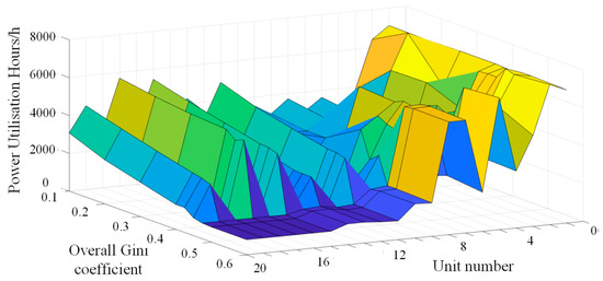
Figure 3.
Annual planned electric generation hour curve of each unit under various overall Gini coefficient values.
Figure 4 shows the total cost of coal consumption for various values of the overall Gini coefficient. As can be seen, the total coal cost decreases as the Gini coefficient increases. When the Gini coefficient value is small, the total cost of coal consumption decreases more quickly as the Gini coefficient increases, and when the Gini coefficient value is greater than 0.4, the total cost of coal consumption decreases slowly as the Gini coefficient increases. Therefore, in this example, 0.4 is the recommended value for the overall Gini coefficient (0.3–0.4 is a fair range as determined by the UN).
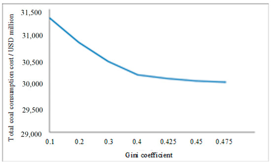
Figure 4.
The total coal consumption cost curve under various overall Gini coefficient values.
It can be seen from the simulation results that the use of this method can reasonably consider the fairness of the annual generation hours of each thermal power unit, while keeping the system parameters constant, which is acceptable to the major power producers. At the same time, the method can better control the coal consumption and pollutant emissions of power generation, which is important for the implementation of the impartial and open dispatching that takes into account coal consumption and environmental benefits.
5.3. Analysis of the Results of the “Planned Electricity” and “Market Electricity” Dual-Track System
Assuming that the odd-numbered units are marketed, the amount of electricity traded directly by each unit is shown in Table 3. In order to simplify the calculation and analysis, it is assumed that a customer with the same market-based unit is equivalent to one customer, i.e., one market-based unit for one directly traded customer. The maximum monthly load for each direct trading customer is shown in Figure 5, and the forecast for other types of units for each month is shown in Appendix A Table A4.
Table 3.
Market energy for power units participated in market transactions.
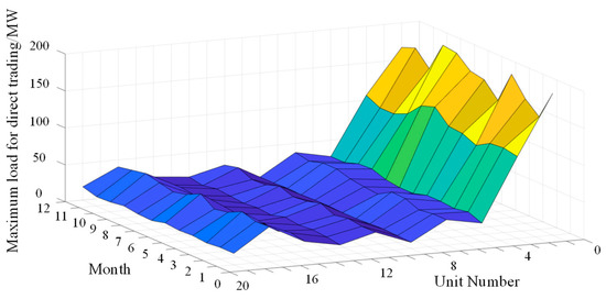
Figure 5.
Maximum load of the Direct trading consumer.
It is assumed that the regulation coefficient kadj is 0.9, the participation incentive coefficient kMarket is 1.1, and the overall Gini coefficient is 0.3; the Gini coefficient of units of the same type is 0.2, and the Gini coefficient of units of the same capacity range is 0.1. The Gini coefficient index of power generation utilization hours of planned electricity after deducting market capacity is 0.6. The converted capacity of each market-based unit for direct trading is shown in Table A5 in the Appendix A.
The total annual electricity consumption, planned electricity consumption, planned electricity generation hours, and total electricity generation hours utilized by each unit are shown in Table A6 in the Appendix A. The overall Gini coefficient value was changed to obtain the total generation hours utilized by each unit for various Gini coefficient values as shown in Figure 6. When the overall Gini coefficient for planned electricity is 0.1, there is a very strict requirement for fairness in the number of generation hours used by each thermal unit. The difference in generation hours between thermal units is relatively small, but there is still some difference between marketed and non-marketed units. As the Gini coefficient value increases, the equity requirement is gradually relaxed and the fluctuation in the number of hours of generation use between units increases. Similar to the results of the conventional scheduling model, the Gini coefficient value is greater than 0.45, and the number of hours utilized by each unit remains the same. This means that the Gini coefficient value of each unit is around 0.45 when the fairness constraint of each unit is not considered.
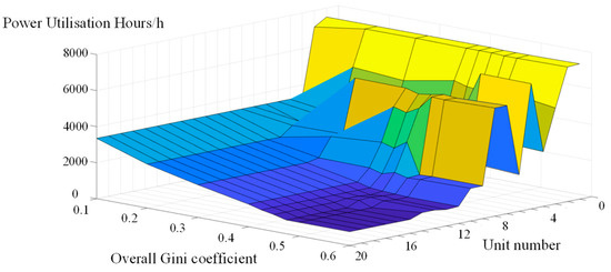
Figure 6.
Annual electric generation hour curve of each unit under different overall Gini coefficient values.
Changing the market participation incentive factor kMarket from 1 to 1.5, the planned electricity and total generation hours of each unit are shown in Table A7 and Table A8 in the Appendix A, respectively. The results in the table show that as kMarket increases, the amount of planned electricity and total generation hours allocated to market-based units increases, while the amount of planned electricity and total generation hours allocated to non-market-based units decreases, which achieves the purpose of adjusting the degree of incentive to participate in market trading by adjusting kMarket.
6. Conclusions
This paper establishes an optimal model for annual electricity scheduling based on the fairness constraint set of the Gini coefficient. The annual electricity of each unit is the decision variable. It can realize the dual-track operation mode of “planned electricity” and “market electricity” for the power grid of high proportion of new energy and fully planned electricity. The annual electricity plan can be formulated as a reasonable manner under the dual-track operation mode of “planned electricity” and “market electricity”, as well as the fully planned electricity mode. The theoretical and numerical analysis shows the following conclusions.
(1) Under traditional planned power dispatch model, the optimal power allocation result is obtained by solving a continuous optimization model. The Gini coefficient, a recognized fairness indicator, is used to constrain the overall power utilization hours of each unit. It can reduce energy, resource consumption, and pollutant emissions. A more fair annual power plan allocation scheme can be obtained. The Annual Electricity Plan (AEP) is designed to focus on different levels of equity by adjusting the Gini coefficient.
(2) Under the dual-track operation mode of “planned electricity” and “market electricity”, the proposed model can take into account the uncertainties of new energy generation such as wind and photovoltaic in a more detailed manner by adding a monthly power balance constraint. It converts the capacity of “market electricity” to take into account the peak and frequency regulation reserve demand on a monthly basis and introducing a fairness constraint set of the Gini coefficient. The optimal allocation of annual power plan is achieved under the dual-track operation mode. By adjusting the Gini coefficient, a balance can be struck between fairness and affordability. By adjusting the market participation incentive coefficient, the level of incentive for market transactions can be effectively controlled.
In this paper, fairness problems for the power generation company, including annual power generation and peaking responsibility are considered. However, fairness of undertaking frequency regulation responsibility for all the generation units should also be considered, which will influence the market capacity conversion results. The annual electricity scheduling considering the frequency regulation fairness is the focus of our following research work.
Author Contributions
Conceptualization and writing—original draft preparation, N.Z. and M.Z.; methodology, J.H.; writing—review and editing, L.S. and J.L.; visualization, W.L. All authors have read and agreed to the published version of the manuscript.
Funding
This research was funded by Science and technology project of State Grid Liaoning Electric Power Co., Ltd., grant number 2021YF-44.
Institutional Review Board Statement
Not applicable.
Informed Consent Statement
Not applicable.
Data Availability Statement
Not applicable.
Acknowledgments
This research was also supported by Liaoning Provincial Public Welfare Research Fund for Science Undertakings in 2021 (Soft Science Research Program).
Conflicts of Interest
The authors declare no conflict of interest.
Appendix A
Table A1.
Unit s’ operation parameter.
Table A1.
Unit s’ operation parameter.
| Unit | Cost of Coal Consumption ($/kWh) | Coal Consumption for Electricity Supply (g/(kWh) | Desulfurization Rate | ||||
|---|---|---|---|---|---|---|---|
| 1 | 500 | 19.073 | 267.022 | 8000 | 3000 | 1300 | 0.99 |
| 2 | 475 | 19.273 | 269.822 | 8000 | 3000 | 1300 | 0.985 |
| 3 | 450 | 20.089 | 281.246 | 8000 | 3000 | 1300 | 0.98 |
| 4 | 425 | 20.189 | 282.646 | 8000 | 3000 | 1300 | 0.975 |
| 5 | 180 | 22.368 | 313.152 | 7000 | 2000 | 1000 | 0.985 |
| 6 | 160 | 22.568 | 315.952 | 7000 | 2000 | 1000 | 0.975 |
| 7 | 135 | 19.213 | 268.982 | 6000 | 1800 | 1000 | 0.985 |
| 8 | 130 | 19.413 | 271.782 | 6000 | 1800 | 1000 | 0.98 |
| 9 | 125 | 19.098 | 267.372 | 6000 | 1800 | 1200 | 0.975 |
| 10 | 120 | 19.298 | 270.172 | 6000 | 1800 | 1200 | 0.97 |
| 11 | 85 | 29.24 | 409.36 | 6500 | 1000 | 600 | 0.975 |
| 12 | 85 | 29.44 | 412.16 | 6500 | 1000 | 600 | 0.97 |
| 13 | 80 | 26.032 | 364.448 | 6200 | 1100 | 700 | 0.965 |
| 14 | 80 | 26.132 | 365.848 | 6200 | 1100 | 700 | 0.97 |
| 15 | 55 | 29.255 | 409.57 | 6000 | 800 | 500 | 0.965 |
| 16 | 52.5 | 29.455 | 412.37 | 6000 | 800 | 500 | 0.975 |
| 17 | 50 | 30.068 | 420.952 | 6000 | 800 | 500 | 0.97 |
| 18 | 47.5 | 30.168 | 422.352 | 6000 | 800 | 500 | 0.965 |
| 19 | 45 | 30.21 | 422.94 | 6000 | 800 | 500 | 0.96 |
| 20 | 42.5 | 30.41 | 425.74 | 6000 | 800 | 500 | 0.955 |
Table A2.
Annual power plan results of each unit in two scenarios.
Table A2.
Annual power plan results of each unit in two scenarios.
| Unit | Scenario 1 | Scenario 2 | ||||||
|---|---|---|---|---|---|---|---|---|
| Hours of Power Generation Utilization | Annual Planned Electricity (MWh) | Total Coal Consumption (Million Tons) | Sulfur Dioxide Emissions (Tons) | Hours of Power Generation Utilization | Annual Planned Electricity (MWh) | Total Coal Consumption (Million Tons) | Sulfur Dioxide Emissions (Tons) | |
| 1 | 7460 | 3,730,000 | 99.60 | 100.38 | 7460 | 3,730,000 | 99.60 | 100.38 |
| 2 | 7460 | 3,543,500 | 95.61 | 143.05 | 7460 | 3,543,500 | 95.61 | 143.05 |
| 3 | 5342 | 2,403,900 | 67.61 | 129.39 | 5776 | 2,599,200 | 73.10 | 139.90 |
| 4 | 3000 | 1,275,000 | 36.04 | 85.78 | 3000 | 1,275,000 | 36.04 | 85.78 |
| 5 | 5342 | 961,560 | 30.11 | 38.82 | 3000 | 540,000 | 16.91 | 21.80 |
| 6 | 2000 | 320,000 | 10.11 | 21.53 | 2000 | 320,000 | 10.11 | 21.53 |
| 7 | 6000 | 810,000 | 21.79 | 32.70 | 5776 | 779,760 | 20.97 | 31.48 |
| 8 | 5342 | 694,460 | 18.87 | 37.38 | 3000 | 390,000 | 10.60 | 20.99 |
| 9 | 3000 | 375,000 | 10.03 | 25.23 | 3000 | 375,000 | 10.03 | 25.23 |
| 10 | 1800 | 216,000 | 5.84 | 17.44 | 2000 | 240,000 | 6.48 | 19.38 |
| 11 | 1000 | 85,000 | 3.48 | 5.72 | 1861 | 1,581,805 | 6.48 | 10.64 |
| 12 | 1000 | 85,000 | 3.50 | 6.86 | 1861 | 1,581,805 | 6.52 | 12.77 |
| 13 | 1100 | 88,000 | 3.21 | 8.29 | 1861 | 148,880 | 5.43 | 14.02 |
| 14 | 1100 | 88,000 | 3.22 | 7.10 | 1861 | 148,880 | 5.45 | 12.02 |
| 15 | 912 | 50,160 | 2.05 | 4.72 | 1861 | 1,023,505 | 4.19 | 9.64 |
| 16 | 1000 | 52,500 | 2.16 | 3.53 | 1861 | 97,703 | 4.03 | 6.57 |
| 17 | 1000 | 50,000 | 2.10 | 4.04 | 1861 | 93,050 | 3.92 | 7.51 |
| 18 | 912 | 43,320 | 1.83 | 4.08 | 1861 | 88,397 | 3.73 | 8.33 |
| 19 | 912 | 41,040 | 1.74 | 4.42 | 1861 | 83,745 | 3.54 | 9.02 |
| 20 | 912 | 38,760 | 1.65 | 4.69 | 1861 | 79,093 | 3.37 | 9.58 |
Table A3.
Annual energy scheduling results of each unit according to the dynamic difference method.
Table A3.
Annual energy scheduling results of each unit according to the dynamic difference method.
| Unit | Hours of Power Generation Utilization | Annual Planned Electricity (MWh) | Total Coal Consumption (Million Tons) | Sulfur Dioxide Emissions (Tons) |
|---|---|---|---|---|
| 1 | 5280 | 2,640,000 | 70.49 | 71.05 |
| 2 | 5280 | 2,508,000 | 67.67 | 101.25 |
| 3 | 5280 | 2,376,000 | 66.82 | 127.89 |
| 4 | 5280 | 2,244,000 | 63.43 | 150.98 |
| 5 | 4367 | 786,060 | 24.62 | 31.73 |
| 6 | 4367 | 698,720 | 22.08 | 47.01 |
| 7 | 4367 | 589,545 | 15.86 | 23.80 |
| 8 | 4367 | 567,710 | 15.43 | 30.56 |
| 9 | 4567 | 570,875 | 15.26 | 38.41 |
| 10 | 4567 | 548,040 | 14.81 | 44.25 |
| 11 | 3049 | 259,165 | 10.61 | 17.44 |
| 12 | 3049 | 259,165 | 10.68 | 20.92 |
| 13 | 3149 | 251,920 | 9.18 | 23.73 |
| 14 | 3149 | 251,920 | 9.22 | 20.34 |
| 15 | 2337 | 128,535 | 5.26 | 12.11 |
| 16 | 2337 | 122,693 | 5.06 | 8.25 |
| 17 | 806 | 40,300 | 1.70 | 3.25 |
| 18 | 806 | 38,285 | 1.62 | 3.61 |
| 19 | 806 | 36,270 | 1.53 | 3.90 |
| 20 | 806 | 34,255 | 1.46 | 4.15 |
Table A4.
Predicted electricity energy for the other type of units.
Table A4.
Predicted electricity energy for the other type of units.
| Month | Wind Power Forecast (MWh) | Nuclear Power Forecast (MWh) | Hydropower Forecast (MWh) | Total Annual Electricity Demand (MWh) |
|---|---|---|---|---|
| January | 1,086,880 | 543,440 | 407,580 | 15,623,970 |
| February | 892,440 | 446,220 | 334,660 | 12,828,810 |
| March | 1,032,040 | 516,020 | 387,020 | 14,835,650 |
| April | 942,300 | 471,150 | 353,360 | 13,545,610 |
| May | 952,280 | 476,140 | 357,100 | 13,689,010 |
| June | 927,340 | 463,670 | 347,750 | 13,330,520 |
| July | 1,032,040 | 516,020 | 387,020 | 14,835,650 |
| August | 1,002,130 | 501,070 | 375,800 | 14,405,630 |
| September | 932,330 | 466,160 | 349,620 | 13,402,220 |
| October | 972,220 | 486,110 | 364,580 | 13,975,620 |
| November | 1,047,000 | 523,500 | 392,620 | 15,050,570 |
| December | 1,141,720 | 570,860 | 428,150 | 16,412,300 |
Table A5.
Market electricity conversion capacity for each unit.
Table A5.
Market electricity conversion capacity for each unit.
| Unit | Direct Trading Converted Capacity (MW) | |||||||||||
|---|---|---|---|---|---|---|---|---|---|---|---|---|
| January | February | March | April | May | June | July | August | September | October | November | December | |
| 1 | 141 | 112 | 124 | 143 | 111 | 126 | 129 | 141 | 143 | 113 | 128 | 123 |
| 3 | 82 | 85 | 82 | 75 | 82 | 83 | 96 | 91 | 77 | 71 | 72 | 78 |
| 5 | 19 | 24 | 21 | 23 | 23 | 18 | 19 | 21 | 26 | 25 | 20 | 20 |
| 7 | 26 | 25 | 24 | 29 | 29 | 21 | 23 | 25 | 29 | 28 | 25 | 28 |
| 9 | 6 | 6 | 7 | 6 | 6 | 6 | 8 | 7 | 6 | 7 | 7 | 5 |
| 11 | 20 | 19 | 22 | 19 | 24 | 21 | 19 | 23 | 18 | 19 | 25 | 21 |
| 13 | 10 | 11 | 14 | 12 | 13 | 10 | 11 | 11 | 11 | 12 | 10 | 13 |
| 15 | 17 | 19 | 15 | 17 | 13 | 15 | 16 | 17 | 16 | 17 | 13 | 16 |
| 17 | 35 | 34 | 38 | 31 | 29 | 37 | 31 | 28 | 31 | 34 | 32 | 29 |
| 19 | 12 | 12 | 11 | 11 | 11 | 12 | 9 | 10 | 11 | 9 | 9 | 12 |
Table A6.
Aunal electricity energy scheduling results under the basic case study scenario.
Table A6.
Aunal electricity energy scheduling results under the basic case study scenario.
| Unit | Total Power Plan (MWh) | Annual Planned Electricity (MWh) | Total Hours Utilized | Planned Electricity Utilization Hours |
|---|---|---|---|---|
| 1 | 35,459,173 | 25,459,174 | 7092 | 6841 |
| 2 | 32,496,427 | 32,496,425 | 6841 | 6841 |
| 3 | 25,534,142 | 19,534,145 | 5674 | 5297 |
| 4 | 11,692,667 | 11,692,662 | 2751 | 2751 |
| 5 | 6,159,929 | 4,359,921 | 3422 | 2751 |
| 6 | 2,934,635 | 2,934,632 | 1834 | 1834 |
| 7 | 7,573,912 | 5,773,916 | 5610 | 5297 |
| 8 | 3,576,585 | 3,576,583 | 2751 | 2751 |
| 9 | 4,094,091 | 3,260,767 | 3275 | 2751 |
| 10 | 2,200,971 | 2,200,976 | 1834 | 1834 |
| 11 | 3,361,590 | 1,094,929 | 3955 | 1707 |
| 12 | 1,450,676 | 1,450,670 | 1707 | 1707 |
| 13 | 2,501,015 | 1,167,677 | 3126 | 1707 |
| 14 | 1,365,345 | 1,365,343 | 1707 | 1707 |
| 15 | 2,499,408 | 666,078 | 4544 | 1707 |
| 16 | 8,960,00 | 896,000 | 1707 | 1707 |
| 17 | 2,631,904 | 298,574 | 5264 | 1707 |
| 18 | 8,106,73 | 810,670 | 1707 | 1707 |
| 19 | 1,544,934 | 584,935 | 3433 | 1707 |
| 20 | 725,335 | 725,335 | 1707 | 1707 |
Table A7.
Annual planned energy of each unit under different encouraged coefficient.
Table A7.
Annual planned energy of each unit under different encouraged coefficient.
| Unit | Planned Power Allocation for Each Unit (MWh) | |||||
|---|---|---|---|---|---|---|
| 1 | 1.1 | 1.2 | 1.3 | 1.4 | 1.5 | |
| 1 | 2,480,828 | 2,530,998 | 2,571,680 | 2,605,343 | 2,633,650 | 2,657,780 |
| 2 | 2,539,143 | 2,501,496 | 2,470,951 | 2,445,689 | 2,424,433 | 2,406,323 |
| 3 | 1,927,912 | 1,942,092 | 1,953,593 | 1,963,104 | 1,971,101 | 1,977,930 |
| 4 | 1,179,911 | 1,162,418 | 1,148,226 | 1,136,486 | 1,126,616 | 1,118,193 |
| 5 | 433,985 | 433,448 | 432,999 | 432,630 | 432,314 | 432,059 |
| 6 | 296,138 | 291,746 | 288,185 | 285,237 | 282,760 | 280,647 |
| 7 | 568,792 | 574,049 | 578,306 | 581,831 | 584,800 | 587,322 |
| 8 | 360,913 | 355,562 | 351,221 | 347,637 | 344,619 | 342,038 |
| 9 | 327,251 | 324,169 | 321,672 | 319,609 | 317,868 | 316,383 |
| 10 | 222,106 | 218,815 | 216,141 | 213,938 | 212,072 | 210,485 |
| 11 | 106,920 | 108,868 | 110,441 | 111,753 | 112,850 | 113,792 |
| 12 | 146,405 | 144,238 | 142,475 | 141,020 | 139,793 | 138,745 |
| 13 | 115,858 | 116,097 | 116,298 | 116,469 | 116,603 | 116,725 |
| 14 | 137,794 | 135,759 | 134,100 | 132,726 | 131,561 | 130,581 |
| 15 | 64,479 | 66,224 | 67,646 | 68,827 | 69,813 | 70,669 |
| 16 | 90,424 | 89,089 | 88,007 | 87,107 | 86,344 | 85,696 |
| 17 | 24,533 | 29,681 | 33,863 | 37,321 | 40,233 | 42,705 |
| 18 | 81,817 | 80,604 | 79,627 | 78,801 | 78,129 | 77,539 |
| 19 | 57,184 | 58,166 | 58,949 | 59,609 | 60,142 | 60,611 |
| 20 | 73,208 | 72,112 | 71,237 | 70,515 | 69,898 | 69,378 |
Table A8.
Annual electric generation hour of each unit under different encouraged coefficient.
Table A8.
Annual electric generation hour of each unit under different encouraged coefficient.
| Unit | Total Power Utilization Hours | |||||
|---|---|---|---|---|---|---|
| 1 | 1.1 | 1.2 | 1.3 | 1.4 | 1.5 | |
| 1 | 6962 | 7062 | 7143 | 7211 | 7267 | 7316 |
| 2 | 5346 | 5266 | 5202 | 5149 | 5104 | 5066 |
| 3 | 5618 | 5649 | 5675 | 5696 | 5714 | 5729 |
| 4 | 2776 | 2735 | 2702 | 2674 | 2651 | 2631 |
| 5 | 3411 | 3408 | 3406 | 3403 | 3402 | 3400 |
| 6 | 1851 | 1823 | 1801 | 1783 | 1767 | 1754 |
| 7 | 5547 | 5586 | 5617 | 5643 | 5665 | 5684 |
| 8 | 2776 | 2735 | 2702 | 2674 | 2651 | 2631 |
| 9 | 3285 | 3260 | 3240 | 3223 | 3210 | 3198 |
| 10 | 1851 | 1823 | 1801 | 1783 | 1767 | 1754 |
| 11 | 3924 | 3947 | 3966 | 3981 | 3994 | 4005 |
| 12 | 1722 | 1697 | 1676 | 1659 | 1645 | 1632 |
| 13 | 3115 | 3118 | 3120 | 3122 | 3124 | 3126 |
| 14 | 1722 | 1697 | 1676 | 1659 | 1645 | 1632 |
| 15 | 4505 | 4537 | 4563 | 4585 | 4603 | 4618 |
| 16 | 1722 | 1697 | 1676 | 1659 | 1645 | 1632 |
| 17 | 5157 | 5260 | 5344 | 5413 | 5471 | 5521 |
| 18 | 1722 | 1697 | 1676 | 1659 | 1645 | 1632 |
| 19 | 3404 | 3426 | 3443 | 3458 | 3470 | 3480 |
| 20 | 1722 | 1697 | 1676 | 1659 | 1645 | 1632 |
References
- Shi, J.; Tan, S. Algorithm of Energy Saving Generation Dispatch Scheduling. Autom. Electr. Power Syst. 2008, 32, 48–51. [Google Scholar]
- Kong, L.; Liu, Q.; Lv, S.; Wang, J.; Yang, Q.; Yang, X. Analysis on Economic Compensation for Energy Saving Dispatch in Jiangsu Province. Electr. Power Surv. Des. 2013, 12, 1–4. [Google Scholar]
- Su, Q.; Ma, Q.; Liu, Y. Research on Implementation and Application of Policy for Energy Conservation and Emission Reduction in Shaanxi Electric Power Company. Shaanxi Electr. Power 2008, 36, 9–11. [Google Scholar]
- Wang, W.; Peng, Y.; Zhang, J.; Shi, S.; Lin, G.; Gao, C. Design of Mechanism to Coordinate Both Energy Conservation and Pollutant Emission Reduction with Power Generation Market in Chongqing Power Grid. Power Syst. Technol. 2009, 33, 93–98. [Google Scholar]
- Shi, S.-H.; Wang, J.-M.; Wang, W.; Kong, Q.-Y.; Zhang, W.-Z.; Tian, J. Annual Energy Schedule Model Based on Dynamic Difference. Power Syst. Technol. 2009, 33, 60–65. [Google Scholar]
- Zhang, L.; Liu, J.Y.; Liu, J.C.; Liu, J.J.; Wu, Z.Y.; Wen, L.L. Study on scheduling and resolution algorithm of annual contract volume for thermal power units. Relay 2007, 35, 64–69. [Google Scholar]
- Ferrero, R.W.; Rivera, J.F. A dynamic programming two-stage algorithm for long-term hydrothermal scheduling of multireservoir systems. IEEE Trans. Power Syst. 1998, 13, 1534–1540. [Google Scholar] [CrossRef]
- Fu, Y.; Shahidehpour, M.; Li, Z. Long-term security-constrained unit commitment: Hybrid Dantzig-Wolfe decomposition and subgradient approach. IEEE Trans. Power Syst. 2005, 20, 2093–2106. [Google Scholar] [CrossRef]
- Ding, J.; Somani, A. A Long-Term Investment Planning Model for Mixed Energy Infrastructure Integrated with Renewable Energy. In Proceedings of the 2010 IEEE Green Technologies Conference, Grapevine, TX, USA, 15–16 April 2010; pp. 1–10. [Google Scholar]
- Zeng, M.; Shi, L.-J.; Dong, J. Study on Issues Reated to Energy-Saving Dispatching of Generation that Conforms to the Market Mechanism. Electr. Power Technol. Econ. 2007, 1, 1–5. [Google Scholar]
- Shang, J. Research on Energy-Saving Generation Dispatching Mode and Operational Mechanism Considering Market Mechanism and Government Macro-Control. Power Syst. Technol. 2007, 31, 55–62. [Google Scholar]
- Shang, J. Comparative Research on Main Energy-Saving Generation Dispatching Model Considering Market Mechanism. Power Syst. Technol. 2008, 32, 78–85. [Google Scholar]
- Hua, Q.; Liu, H.; Hu, Z. User interest distribution pattern measurement method based on Gini coefficient. Comput. Eng. 2012, 38, 39–42. [Google Scholar]
- Xu, W.; Jiang, Z.; Ruan, L. Analysis of Gini coefficient of property income between urban and rural residents in China. Sci. Mosaic 2015, 12, 160–165. [Google Scholar]
- Wang, J.-N.; Lu, Y.-T.; Zhou, J.-S.; Li, Y. Analysis of China resource-environment Gini coefficient based on GDP. China Environ. Sci. 2006, 26, 111–115. [Google Scholar]
- He, Z.; Qin, P.; Ruan, C.; Xie, M.; Susan, M. Lorenz curve and its application in plant ecology. J. Nanjing For. Univ. Nat. Sci. Ed. 2004, 28, 37–41. [Google Scholar]
- Wang, H.; Zhu, J. Robustness analysis of wind power grid based on the Gini coefficient of load ratio. Renew. Energy Resour. 2016, 34, 208–213. [Google Scholar]
- Dai, J.L.; Wang, P.; Wang, X.; Qi, J. Discussion on impartiality index of power dispatching based on Gini coefficient. Autom. Electr. Power Syst. 2008, 32, 26–29. [Google Scholar]
- Xiong, J. A comparative study of Gini coefficient estimation methods. Stud. Financ. Econ. 2003, 1, 79–82. [Google Scholar]
- Hu, Z. Research on the best value of Gini coefficient theory and its simple calculation formula. Econ. Res. 2004, 9, 60–69. [Google Scholar]
- Zhu, B. Research on China’s Gini Coefficient. Ph.D. Thesis, Southwestern University of Finance and Economics, Chengdu, China, 2014. [Google Scholar]
- Hayashi, D. Harnessing innovation policy for industrial decarbonization: Capabilities and manufacturing in the wind and solar power sectors of China and India. Energy Res. Soc. Sci. 2020, 7, 101644. [Google Scholar] [CrossRef]
- Eryilmaz, S.; Kan, C. Reliability based modeling and analysis for a wind power system integrated by two wind farms considering wind speed dependence. Reliab. Eng. Syst. Saf. 2020, 203, 107077. [Google Scholar] [CrossRef]
- Kim, K.J.; Lee, H.; Koo, Y. Research on local acceptance cost of renewable energy in South Korea: A case study of photovoltaic and wind power projects. Energy Policy 2020, 144, 116684. [Google Scholar] [CrossRef]
- Zhang, C.; Wang, X. Impartiality Indexes of Power Dispatching Based on Modified Weighed Coefficient of Variation. Electr. Power Technol. Econ. 2009, 21, 5–9. [Google Scholar]
- Zeng, F.; Wang, P. Fairness Coefficient Analysis of Power Dispatching in North China Area. Mod. Electr. Power 2010, 27, 78–81. [Google Scholar]
Publisher’s Note: MDPI stays neutral with regard to jurisdictional claims in published maps and institutional affiliations. |
© 2022 by the authors. Licensee MDPI, Basel, Switzerland. This article is an open access article distributed under the terms and conditions of the Creative Commons Attribution (CC BY) license (https://creativecommons.org/licenses/by/4.0/).