On Hourly Forecasting Heating Energy Consumption of HVAC with Recurrent Neural Networks

Abstract

Optimizing the heating, ventilation, and air conditioning (HVAC) system to minimize district heating usage in large groups of managed buildings is of the utmost important, and it requires a machine learning (ML) model to predict the energy consumption. An industrial use case to reach large building groups is restricted to using normal operational data in the modeling, and this is one reason for the low utilization of ML in HVAC optimization. We present a methodology to select the best-fitting ML model on the basis of both Bayesian optimization of black-box models for defining hyperparameters and a fivefold cross-validation for the assessment of each model’s predictive performance. The methodology was tested in one case study using normal operational data, and the model was applied to analyze the energy savings in two different practical scenarios. The software for the modeling is published on GitHub. The results were promising in terms of predicting the energy consumption, and one of the scenarios also showed energy saving potential. According to our research, the GitHub software for the modeling is a good candidate for predicting the energy consumption in large building groups, but further research is needed to explore its scalability for several buildings.

1. Introduction

Ever stricter CO₂ emissions targets pose a challenge for buildings which contribute a major part of the global carbon dioxide emissions in cities [1], with heating being the largest contributor in the northern countries [2]. According to the Confederation of Finnish Construction Industries, 25% of energy consumption and 30% of greenhouse gas emissions in Finland originate from buildings [2]. Accordingly, building owners are required to implement proactive actions to meet national targets by improving energy efficiency. In Finland, the Ministry of the Environment has stated a goal of 55% reduction for the energy consumption of buildings compared to levels in 2005 [3]. The actions instituted in the strategy are estimated to reduce greenhouse gas emissions of heating in buildings by 92%. These procedures play an essential role in climate change mitigation. District heating systems are seen as a vehicle for achieving energy efficiency targets, and in Europe, especially, district heating systems play an important role in the energy systems [4]. The reason behind this is that district heating is flexible regarding its energy sources; therefore, renewables can be used as a fuel in district heating plants.

However, the energy usage in buildings is complex due to the fact that the buildings are of various types and ages, with owners who have diverse values, lifestyles, and ways of using buildings [5,6]. This results in a fragmented field with multiple actors embedded in the building value chain, including designers and architects, developers and capital providers, contractors, engineers, building owners, and tenants [7]. In addition to this, the used technologies have a very long life cycle [5] and, therefore, the renovation cycle is relatively long. Investments in new technology to improve energy efficiency will be important to achieve the stated goals of energy reduction, and one typical investment to reduce CO₂ emissions would be to move toward heating technologies like district heating with more environmentally friendly fuels. These types of investments are typically very large and expensive. However, there are also low-cost investments compared to these large ones such as using digitalization to optimize the use of current technologies [8,9]. Digitalization can be used to optimize the existing district heating systems, but the energy consumption reduction is milder. Therefore, it will be important to scale up the usage of digitalization to include multiple buildings to achieve more significant impacts.

One major trend in the transition toward using digitalization is to utilize machine learning (ML) to optimize operations. In the European Union, the Energy Performance of Buildings Directive (EPBD) and the Energy Efficiency Directive have been revised to increase the intelligence in the buildings, because this can have major impact on improving the energy efficiency [8]. On the other hand, ML algorithms, as a means to increase the intelligence, are highly suitable for improving energy efficiency in the case of district heating because they can learn the unique dynamic behavior of specific buildings, and this information can be used to tune existing district heating systems to be as optimum as possible in terms of energy efficiency. The behavior of individual buildings varies substantially due to the different technologies used and due to the different usage of the buildings. The increase in renewables on the supply side has created the desire to have more flexible demand [10], which can be achieved by modeling the dynamic behavior of the buildings. Thus, adjusting the operations of heating, ventilation, and cooling (HVAC) equipment is expected to have a major impact on energy reduction [10].

There are some solutions on the market which claim to allow smart control (SC). However, the authors’ understanding based on several discussions with experts is that the role of ML is minimal, if there is any role at all in such solutions. Nevertheless, these solutions are in commercial use, and they definitively provide a certain added value to their customers.

The usage of SC was analyzed using the real-life data of 109 district heating customers [3,4,11]. The data included 31 customers who implemented SC in their operations and 78 customers who did not implement it, used as a reference group. The data analyzed were for four years (2014–2017), and the SC actions started in 2016. According to results, for the year 2016, the normative heat consumption was 7.1% smaller compared to the level in 2014 for SC buildings, whereas the heat consumption increased by 1.7% for the reference buildings. Furthermore, the energy bills were smaller for customers who implemented SC by an average of 5% in 2017 compared to the level in 2014; however, for the reference buildings, the energy bill increased by 1% for the same period.

According to the literature, ML has been used in several research projects to optimize HVAC, and ML is typically used as a supervisory control to define setpoints for the upper-level control [12]. The setpoints are typically temperature values for the internal radiator network and ventilation network. ML is used to model the unique behavior of a specific building, and this model is then used for optimization for different goals. For example, these goals could include minimizing the overall energy consumption or operational cost while ensuring that the indoor air quality parameters such as the temperature and CO₂ levels are within defined tolerances [13]. According to several studies, ML-based supervisory control has succeeded in reducing the overall energy consumption or operational costs from 7% to more than 50% [14,15,16,17,18].

ML based supervisory controls are successful for complex systems implemented by academia, but fail to satisfy industrial users [12,19]. Industry has been very reluctant to adapt complicated ML-based control of HVAC systems; therefore, HVAC systems still use very simple control strategies. The abovementioned SC solutions are still very rare, and ML is not really used properly in these applications. Our research aimed to find answers to questions which would make it easier for industrial players to start using more advanced ML-based supervisory control of HVAC systems.

ML model development starts from data gathering. Data gathering in an industrial environment has several practical restrictions compared to the research environment. First, the data need to be gathered from real buildings, restricted to collecting comprehensive data around a normal operating point. ML algorithms require rich input data covering the whole optimization space in which the model can be used to optimize energy consumption which may be outside the normal operation range. Therefore, our research questions were as follows:

• What would be the optimum ML model structure for energy consumption?
• How good are the district heating energy consumption predictions made by ML algorithms for the HVAC system of the pilot location using normal operational data?
• Can we use an ML model to estimate the energy saving in some scenarios?

This study was mostly performed as part of Iivo Metsä-Eerola’s MSc work [20].

2. Materials and Methods

2.1. Data

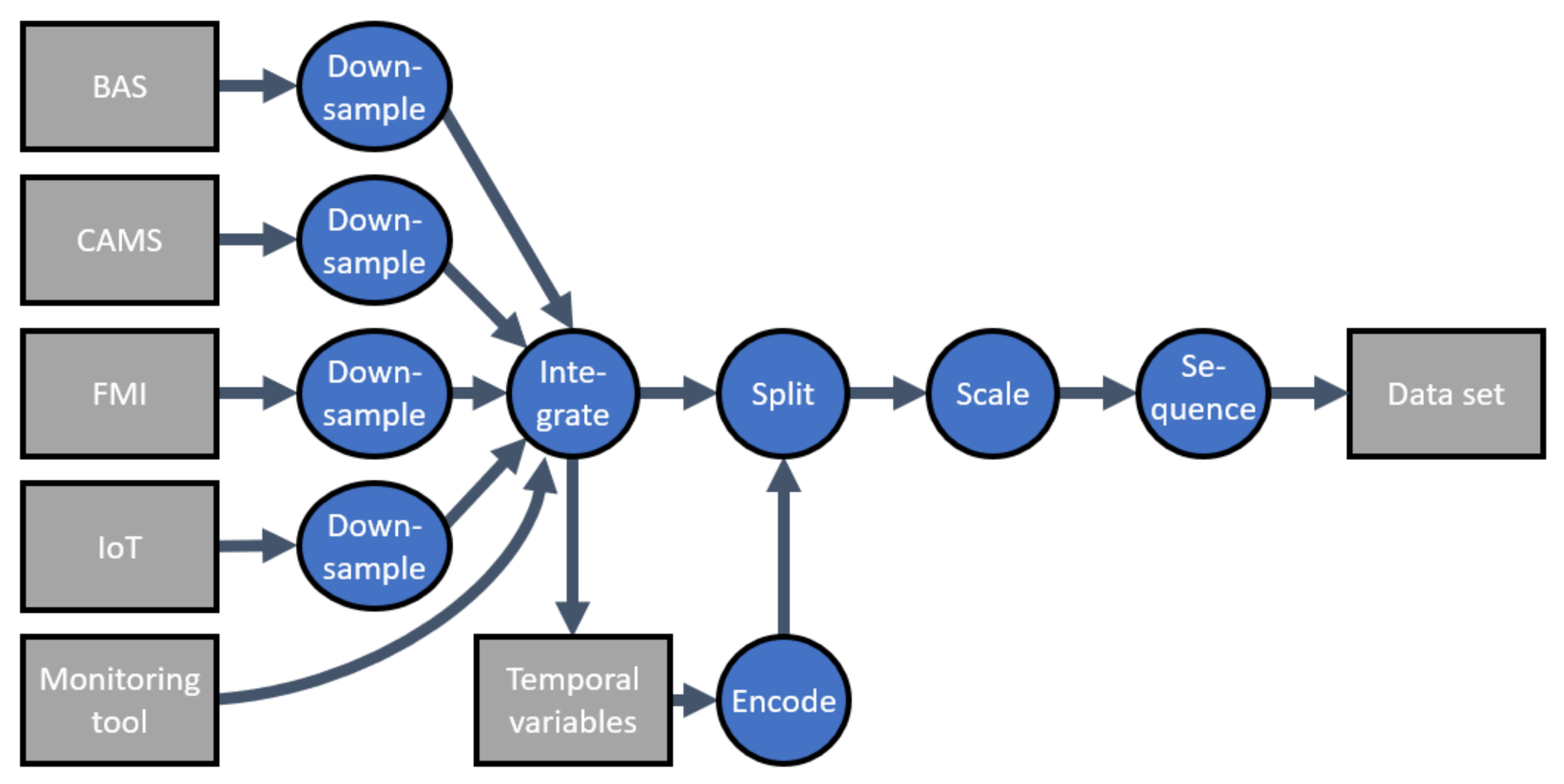
The pilot location analyzed in this study was a large school building spanning 7187 ${\mathrm{m}}^2$ on two stories. The building was opened in 1964 and renovated in 1990. The data were collected in one contiguous interval from 11 February 2021 to 2 May 2021. The data originated from five separate sources: the building automation system (BAS) of the pilot location, the European Union’s Copernicus Atmosphere Monitoring Service (CAMS), Internet of things (IoT) sensors mounted on site, and a district heating energy consumption monitoring tool.

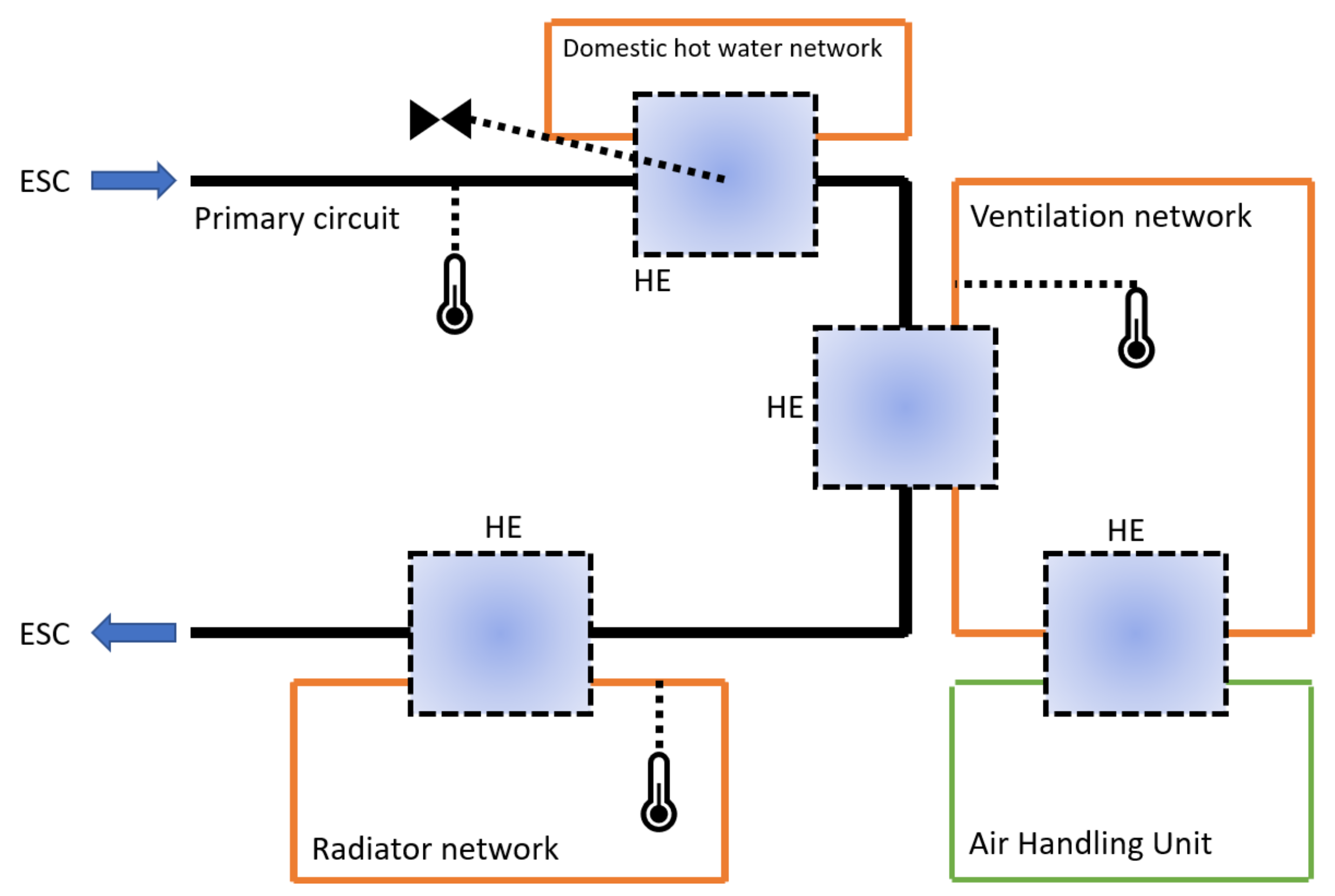
The HVAC system of the pilot location consisted of two heat exchange centers both serving three subsystems, i.e., radiator, ventilation, and domestic hot water networks. From the radiator and ventilation networks, the network temperatures were utilized in the modeling, i.e., “water temperature of radiator network 1 and 2” and “water temperature of ventilation network 1 and 2”. As for the domestic hot water networks, data from the flow valve position controlling the amount of district heat flowing to the heat exchangers were included in the modeling, i.e., “valve of domestic hot water 1 and 2”. Additional parameters from the HVAC system included in the modeling were the temperature of the incoming district heat and the 24 h rolling average of outside temperature. For the carbon dioxide concentration, which is a great proxy variable for building occupancy, observations were collected via IoT sensors mounted on site, and average CO₂ concentrations were utilized in the modeling. Figure 1 shows the locations of the measurements in a simplistic HVAC diagram.

In addition to the average outside temperature parameter obtained from the BAS, two weather parameters were utilized in the modeling: the solar irradiance and outside air relative humidity. From the EU CAMS data, the solar irradiance defined as the power per unit area in electromagnetic radiation was included. These satellite-based observations were calculated considering cloud cover, aerosol optical properties, and ground elevation (Copernicus Atmosphere Monitoring Service, n.d.). The outside air relative humidity observations were downloaded from the API of the Finnish Meteorological Institute (FMI). The FMI weather station which provided the humidity data for this project was located approximately 5 km in a straight line from the pilot destination (Finnish Meteorological Institute, 2021).

Having introduced the input data sources, the only data source not addressed is that producing the target values for the district heating energy consumption. These values were received from the energy consumption monitoring tool of the building owner, used as a basis for invoicing from the district heat supplier, thus including total energy consumption. As these values were obtained in hourly temporal intervals, all the input parameters needed to be down-sampled to the same interval. Down-sampling was the first step of data preprocessing, as presented in Figure 2.

After down-sampling all the input data sources to hourly temporal granularity, the input and target variables were integrated on the basis of timestamps into a single table. The timestamps were then used for the extraction of two temporal variables: the hour of the day and day of the week. A summary of all the input features is presented in

Table 1. Input and target features by uses, sources, and units.

Features	Use	Source	Unit
District heating energy consumption	Target	Monitoring tool	kWh
Valve of domestic hot water network 1	Input	BAS	%
Valve of domestic hot water network 1	Input	BAS	%
Water temperature of incoming district heat	Input	BAS	°C
24 h rolling average of outside temperature	Input	BAS	°C
Water temperature of ventilation network 1	Input	BAS	°C
Water temperature of ventilation network 2	Input	BAS	°C
Water temperature of radiator network 1	Input	BAS	°C
Water temperature of radiator network 2	Input	BAS	°C
$\mathrm{Average} \mathrm{facility} {\mathrm{CO}}_2$ concentration	Input	IoT	ppm
Outside air relative humidity	Input	FMI	%
Solar irradiance	Input	CAMS	$\frac{\mathrm{W}}{{\mathrm{m}}^2}$
Hour of the day	Input	Timestamp	h
Day of the week	Input	Timestamp	d

. These cyclical variables were encoded using sine and cosine functions to make them more easily interpretable for ML algorithms [21].

After encoding the temporal variables, the data preprocessing continued in three sequential phases: splitting, scaling, and sequencing. Splitting the data into training and testing sets was performed with a nonrandom 80:20 sequential split [22]. The first 20% of the data collection period was chosen for testing, as the latter 80% included a period of manual scenario testing with HVAC controls. It was a priority to include this period of diverse data in the training set.

Scaling of input features to the same scale enables distance-based learning methods to learn equally from each parameter and speeds up convergence of artificial neural networks as used in this study [22]. As a result, min–max scaling of the features was applied. Every instance of a feature was scaled as follows:

$$x_{i.j,scaled} = \frac{x_{i,j} - x_{min}}{x_{max} - x_{min}}\left(b - a\right) + a,$$

where $x_{min}$ and $x_{max}$ represent the minimum and maximum values of the feature, and $x_{i,j}$ represents the non-scaled i-th instance of feature j. The intended scale which the feature is transformed to is depicted with $\left[a,b\right]$. In this study, the applied scale ranged from 0 to 1. The practical implementation of min–max scaling was performed using the Python package scikit-learn [23].

As seen from Figure 2, the last phase of preprocessing was sequencing. Sequencing is required as most of the ML algorithms examined in this study were sequence-based recurrent neural networks (RNNs). The sequencing method applied in this study is called windowing, as the sampling function features a window of a desired length sliding on the temporal axis. After saving one sequence, the window slides one step forward on the temporal axis. This results in a dataset where subsequent observations have all but the most recent data point in common. For input datasets of static ML algorithms, sequencing is not necessary as these use data from a single time instance to formulate a forecast. The lengths of preprocessed datasets are presented in

Table 2. Training and testing input dataset dimensions for difference sequence lengths. The testing samples are of equal length to enable valid comparisons.

Sequence Length	Training Sample	Testing Sample
1	[1555, 15]	[376, 15]
4	[1552, 4, 15]	[376, 4, 15]
8	[1548, 8, 15]	[376, 8, 15]
12	[1544, 12, 15]	[376, 12, 15]

. The predicted variable was to be forecasted 1 h into the future and was, therefore, sampled at the next timepoint following an input sequence.

2.2. Modeling

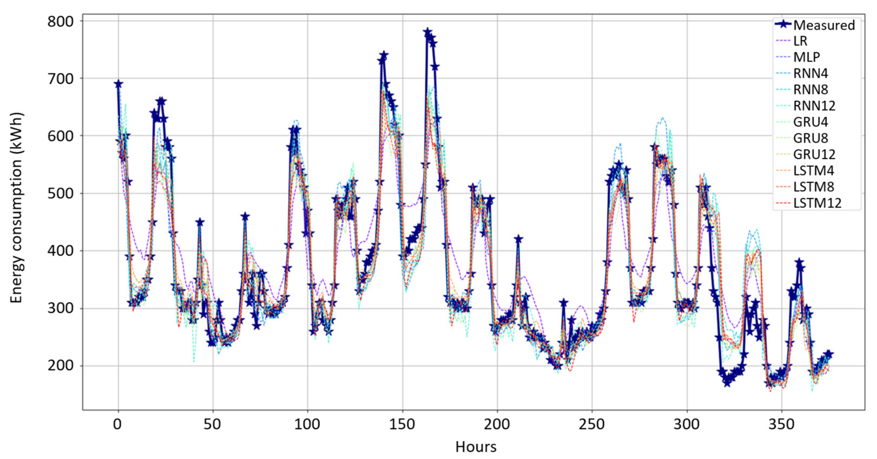
In this study, five model types were examined for the short-term forecasting of district heating energy consumption. Out of these five, three were RNNs with varying cell types, one was the vanilla neural network multilayer perceptron, and one was ordinary least squares estimated linear regression. RNN models with each cell type were tested with three different sequence lengths, as seen in Table 2. Thus, the total number of models tested in this study was 11.

2.2.1. Linear Regression

Linear regression is one of the most common algorithms used in statistical analyses, which is based on the idea that there exists a linear relationship between explanatory and response variables [24]. The general form of a single output linear multivariate regression model is

$$y = \beta X + ϵ,$$

where y is the response variable vector of size m, β is the coefficient vector of size n, X is the data vector of size, and ε is the noise vector of size m. One of the most widespread methods to find the greatest fit producing vector β is the least squares method, which minimizes the squared residuals of points around the curve (Maulud and Abdulazeez, 2020). In contrast to iterative or heuristic methods used commonly in ML, the least squares method is a statistical approach to model training.

2.2.2. Artificial Neural Networks

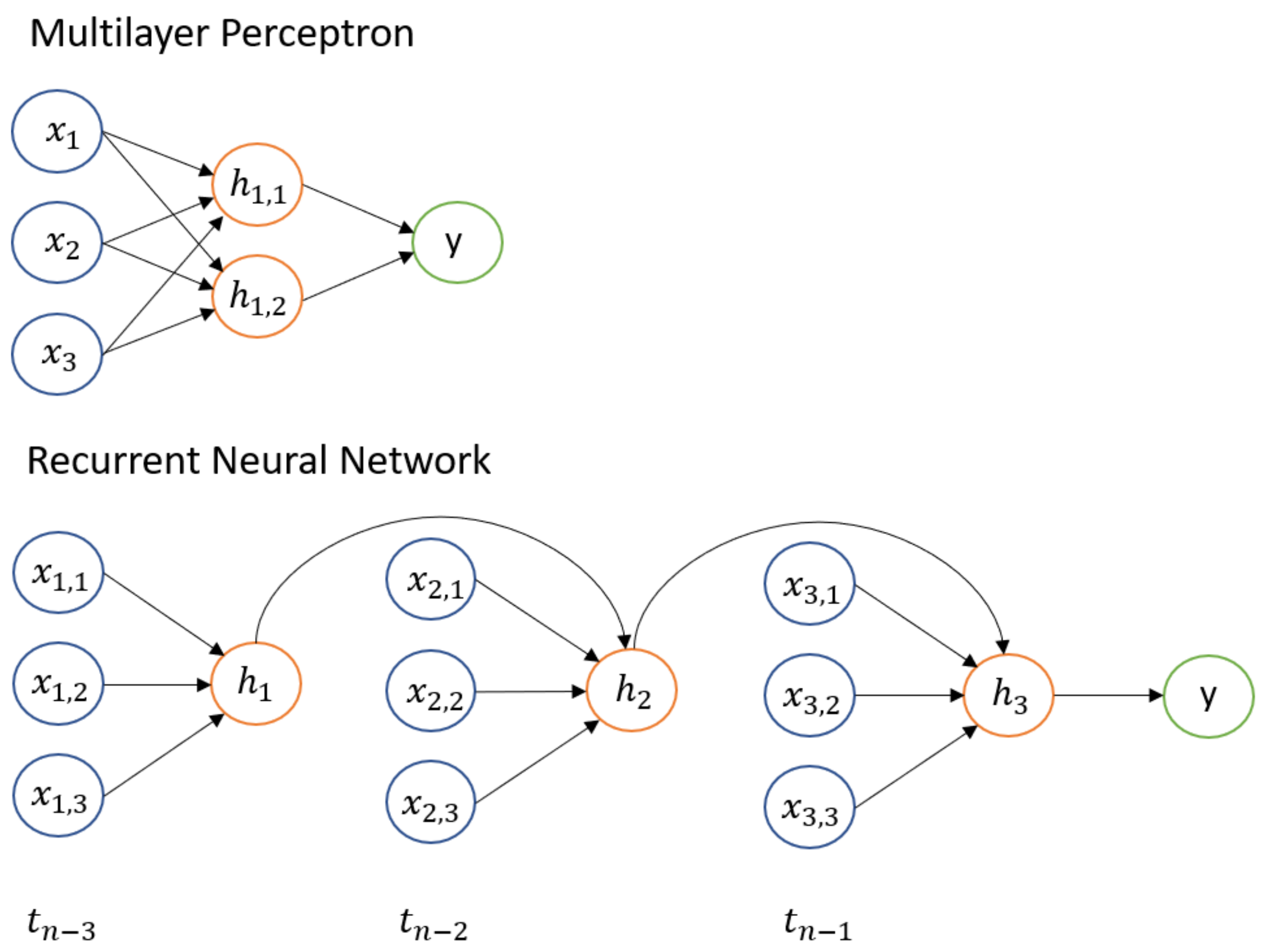
Artificial neural networks (ANNs) are a family of ML models with a structure of a grid connecting nodes of multiple layers capable of conveying transformed information to each other. These networks have been proven to be capable of learning to forecast the behavior of systems by altering the flow of information between the network layers [25]. In this study, two types of ANNs, which differ in the way that information flows in the network, were studied: multilayer perceptron (MLP) and recurrent neural networks (RNNs). In the former, also called a feedforward neural network, information moves solely forward through the network [26]. In the latter, information is fed not only through the network but also through a time sequence as a hidden state. In other words, every forecast made with an RNN requires a sequence of data, whether that sequence is defined in time, space, or some other dimension. The key differences in the basic structure between MLPs and RNNs are shown in Figure 3.

2.2.3. Multilayer Perceptron

As seen in simplistic form in Figure 3, an MLP network consists of input, hidden, and output layers. The mathematical operations of these hidden layers are expressed as

$$h_j = g\left(W_j{h}_{j - 1} + b_j\right),$$

(1)

where $h_j$ describes the output of hidden layer j, $W_j$ describes the weight matrix of hidden layer j, and $b_j$ represents the bias vector of layer j. The contents of matrices W and b are model parameters to be modified during training. The sizes of matrices W and b depend on the sizes of the previous and following layers as the MLP structure necessitates full connectivity between nodes of subsequent layers. Notation g portrays the activation function applied to linearly transformed layer inputs $h_{j - 1}$ used to increase the network’s ability to learn complex patterns [27]. In this study, two different activation functions for MLPs were tested, rectified linear units [28] and the hyperbolic tangent (tanh).

2.2.4. Recurrent Neural Networks

Unlike feedforward MLPs, RNNs capture relationships not only from input data but also from the internal state of previous cells in the sequence. The basic structure of operations in a single RNN cell is visible in the equation of a hidden state as depicted below [25].

$$h_t = g\left(W{x}_t + U{h}_{t - 1} + b\right),$$

where $x_t$ of size $m$ represents the input data vector at time t in the sequence, $h_{t - 1}$ is the output of previous cell (hidden state) of size n, and $U$ is the weight matrix applied to the hidden state of the previous cell. The weights of matrices W, U, and b, sized $n\times m$, $n\times n$, and $n\times 1$, are shared through the whole sequence length [26]. In other words, parameters applied in transformations in n units are repeated in t cells.

Algorithms used for training neural networks are typically based on the backpropagation of gradients. However, modeling long-term dependencies on the backpropagation of gradients is difficult, as the algorithms suffer from exploding and vanishing gradients [29]. These phenomena distort the relationships in the data which the algorithm is trying to capture. One way to battle the issue is to design a more sophisticated activation function for the RNN units to replace common hyperbolic tangent or rectified linear units [30]. Next, two of these are presented: the long short-term memory (LSTM) unit and the gated recurrent unit (GRU).

2.2.5. Long Short-Term Memory

First introduced in [31], LSTMs implement two key innovations to combat gradient-related issues in learning: gates and memory. These structures enable the LSTM cell to regulate the reservation and transmission of information in units. In an LSTM cell, input and forget gates regulate the updating of the internal memory c of size n in LSTM units [30]. Input gates control the addition of new information, while forget gates do the same for forgetting, as expressed below.

$$c_t = f_t{c}_{t - 1} + i_t{\tilde{c}}_t,$$

where f and i are forget and input gates, respectively, and $\tilde{c}$ is the candidate value vector of size n for new cell state. The values of the gates are calculated as

$$f_t = \sigma \left(W_f{x}_t + U_f{h}_{t - 1} + V_f{c}_{t - 1}\right),$$

$$i_t = \sigma \left(W_i{x}_t + U_i{h}_{t - 1} + V_i{c}_{t - 1}\right),$$

where $V_{f,i}$ are diagonal matrices of size $n\times n$, and the activation function $\sigma :ℝ\to \left[0,1\right]$ is the sigmoid function [32]. The candidate solution is calculated on the basis of the inputs and the hidden state

$${\tilde{c}}_t = g\left(W_c{x}_t + U_c{h}_{t - 1}\right),$$

which includes the activation function g defined as either a hyperbolic tangent or rectified linear unit (ReLU) in recent studies [30,33].

The memorized content in cell state c is then applied to the hidden state h through the output gate o as follows:

$$o_t = \sigma \left(W_o{x}_t + U_o{h}_{t - 1} + V_o{c}_t\right).$$

The final hidden state is the activation of $\sigma$ with the input of cell state c regulated by the output function o.

$$h_t = o_{t}g\left(c_t\right).$$

This implementation presented in [34] is slightly different from the original one proposed by Hochreiter and Schmidhuber. Another simpler variant of LSTM is the gated recurrent unit which is presented next.

2.2.6. Gated Recurrent Unit

A gated recurrent unit (GRU) is an LSTM cell variant applied to machine translation [35]. It resembles LSTM in the way that gates control the flow of information. GRU does not include a cell state c; however, it does use past information in hidden state h to update $\tilde{h}$ as follows:

$$\widetilde{h_t} = g\left(W{x}_t + U\left(r_t\odot h_{t - 1}\right)\right),$$

where $\odot$ is the notation for the element-wise product. The reset gate $r_t$ controls how much information is retained from the previous hidden state $h_{t - 1}$ to the new hidden state $h_t$. The value of the reset gate is calculated from the input and previous hidden state.

$$r_t = \mathsf{\sigma }\left(W_r{x}_t + U_r{h}_{t - 1}\right).$$

The new hidden state $h_t$ is then combined from the candidate state $\widetilde{h_t}$ and $h_{t - 1}$.

$$h_t = \left(1 - z_t\right)h_{t - 1} + z_t\widetilde{h_t},$$

where $z_t$ is the update gate balancing the previous hidden state and the current candidate solution. The value of the update gate $z_t$ is calculated similarly as the reset gate $r_t.$

$$z_t = \mathsf{\sigma }\left(W_z{x}_t + U_z{h}_{t - 1}\right).$$

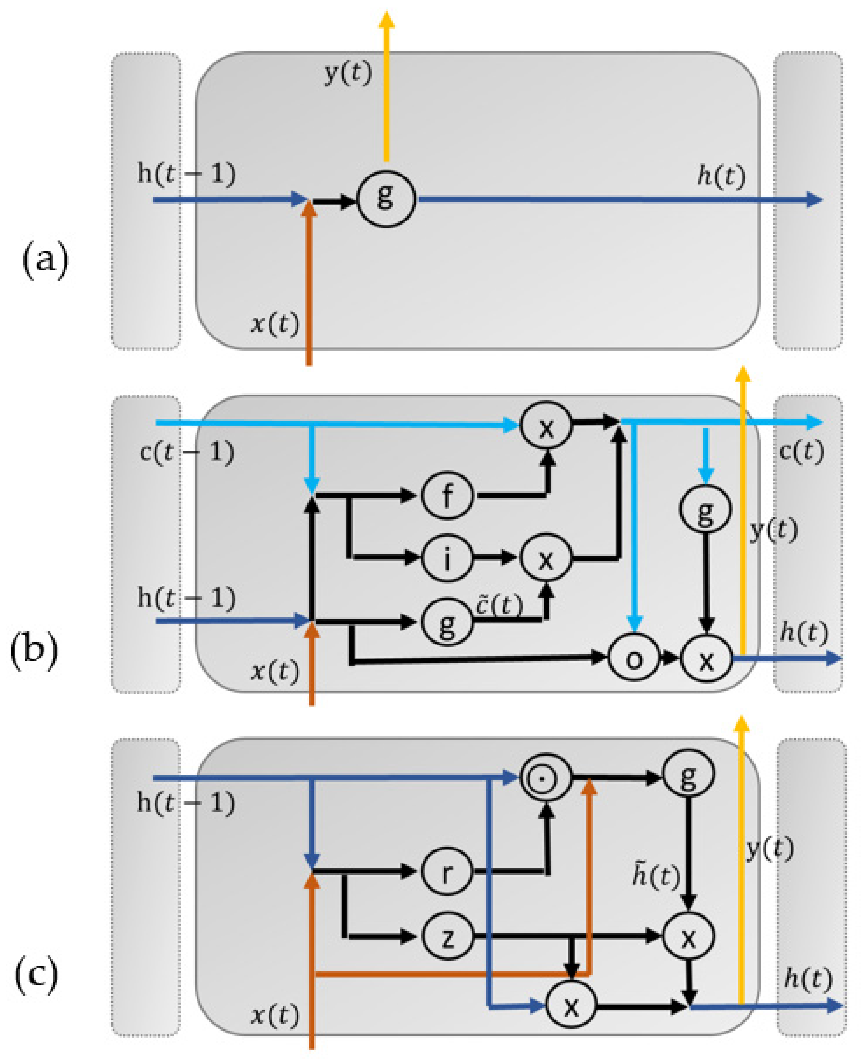
Figure 4 illustrates the differences between the RNN units presented in this study.

2.2.7. Loss Function, Backpropagation of Gradients, and Gradient Descent

Training a neural network to make accurate predictions necessitates penalizing parameter combinations which produce unsatisfactory results. One method to penalize prediction errors $e = \widehat{y} - y$ is a loss function $L\left(\widehat{y},y\right)$. On the basis of the value of the loss function, gradients for network parameters are then calculated with the backpropagation algorithm introduced in [36]. After obtaining the gradients for network parameters, an optimization algorithm is applied to steer the learning process toward the loss function minimizing network parameters. One widely applied optimization algorithm is the stochastic gradient descent (SGD)

$${\mathsf{\theta }}_{t + 1} = {\mathsf{\theta }}_t - \mathsf{\lambda }{\nabla }_{\mathsf{\theta }}L\left(x_t,\mathsf{\theta }\right),$$

where $\mathsf{\lambda }$ is the size of the step in the algorithm, ${\mathsf{\theta }}_i$ are the parameters of the network, and ${\nabla }_{\mathsf{\theta }}L\left(x_t,\mathsf{\theta }\right)$ are the gradients of parameters [31]. The algorithm is based on the idea that constant updates executed on the parameters for each data point will eventually guide the network to the minimum of the loss function [36]. Repeated updates of the SGD algorithm typically lead to a streaky convergence with major variance in the values of the loss function [37].

To combat the streaky convergence of SGD, a mini-batch gradient descent is implemented in this study. In a mini-batch gradient descent, the parameters of the network are updated every n data point in training, which are called mini-batches. In this study, for hyperparameter tuning, the mini-batch size implemented was 32, adhering to the default value provided by the ML Python library TensorFlow [38] and the same as the length of the training data for accelerated retraining.

For noisy objective functions, such as the loss function in SGD, more sophisticated methods in addition to mini-batches are required to ensure convergence. In this study, the efficient first-order optimization algorithm Adam introduced in [39] was implemented for the optimization of neural networks. Adam combines key innovations from other SGD variants such as momentum [40], AdaGrad [41], and RMSProp [42] to form an adaptive solution for a gradient descent. In this study, the Adam algorithm was implemented with default parameter values of ${\beta }_1 = 0.9$, ${\beta }_2 = 0.999$, and $ϵ = 1\cdot {10}^{ - 7}$. The value of the learning rate $\mathsf{\lambda }$ was optimized in a hyperparameter optimization.

2.2.8. Batch Normalization

One problematic phenomenon in ML is the internal covariate shift, which occurs when the input distribution of the network changes from previous instances [43]. This is harmful for the learning process as the model is required to adapt to changes in the input distribution. While an internal covariate shift in the network inputs can be neutralized by domain adaptation methods, inputs to hidden layers deeper in the network experience the same issues [44].

One solution to the internal covariate shift in the inputs of the networks’ inner layers is batch normalization, as introduced in [44]. In batch normalization, the input vector a of each mini-batch is normalized separately based on mini-batch statistics.

$${\mathsf{\mu }}_B = \frac{1}{m}{\sum }_{i = 1}^m{a}_i, {\mathsf{\sigma }}_B^2 = \frac{1}{m}{\sum }_{i = 1}^m{\left(a_i - {\mathsf{\mu }}_B\right)}^2, \widehat{a_i} = \frac{a_i - {\mathsf{\mu }}_B}{\sqrt{{\mathsf{\sigma }}_B^2 + ϵ}}, \mathrm{and} y_i = \mathsf{\gamma }\widehat{a_i} + \mathsf{\delta },$$

where $a_i$ is the initial output of the previous hidden layer, $ϵ$ is a small constant to avoid divisions by zero (0.001 in this study), γ and δ are trainable variables, and $y_i$ is the input of the following hidden layer. When using the model in forecasting, trainable parameters γ and δ are not used as the output of the model must be deterministic. Furthermore, mini-batch-specific statistics for the mean and variance are replaced by population-specific ones. Thus, the input of the following hidden layer is calculated as

$$\widehat{a} = \frac{a - \mathrm{E}\left[a\right]}{\sqrt{\mathrm{Var}\left[a\right] - ϵ}},$$

where $\mathrm{Var}\left[a\right] = \frac{m}{m - 1}{E}_B\left[{\mathsf{\sigma }}_B^2\right]$ is the unbiased estimate for the population variance based on the variances of mini-batches of size m [44].

In addition to removing the adverse effects of the internal covariate shift from the training of a deep neural network, batch normalization works as a regularization method through the random selection of mini-batches [44]. Thus, batch normalization effectively replaces the need for common dropout [45] regularization. Regularization is further addressed in the next section.

2.2.9. Regularization

Regularization methods are required for ML algorithms to be of such efficiency and complexity that they can effectively memorize the whole training dataset. Training an ML algorithm to that length is called overfitting the model to the training data. If this phenomenon occurs, it will make the model poor for use in predicting outcomes on the basis of unseen input data [26]. After all, the goal of the optimization algorithm is to minimize both training and testing errors for the ML model [26] (p. 110).

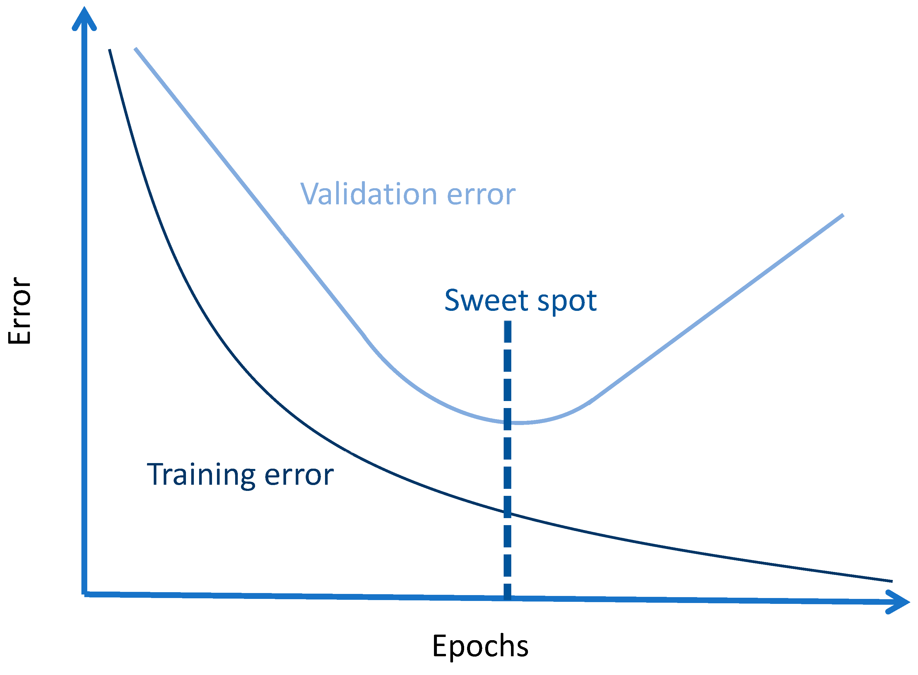
Luckily, overfitting the model does not happen in an instant but rather gradually as more and more epochs or the number of iterations over the training dataset are fed into the modeling algorithm. This phenomenon is shown in Figure 5, where the training and validation errors of a ML model are presented as functions of epochs [46]. The dashed line represents the sweet spot where the training should be stopped before the algorithm starts to overfit, which is visible as the increasing validation error.

This method of halting the training process before overfitting is called early stopping. It is one of the most common regularization techniques due to both its simplicity and its effectiveness [26] (p. 247). The technical implementation of early stopping usually includes a patience parameter which regulates how many epochs of increased validation errors the algorithm tolerates before interrupting the process. After the training has been stopped, the parameters which produce the lowest validation error are then restored. In this study, the patience parameter was set to 20 epochs while the initial training epoch number was 1000.

2.3. Model Tuning

In this study, the term model tuning signifies the process in which the search for the optimal configuration of the ML model hyperparameters is combined with the assessment of each model’s predictive performance. The former objective was achieved via a Bayesian optimization of black-box models, while the latter was achieved by applying a fivefold cross-validation. These methods are introduced next in this study.

2.3.1. Cross-Validation

Cross-validation is a heuristic testing model based on repeated training and validation of nonoverlapping data splits [26] (p. 122). The average validation performance across the splits is then compared to that achieved with other model configurations. Cross-validation is a popular technique as it has minimal assumptions and wide applications for a wide range of different model algorithms [47]. Figure 6 illustrates three sampling processes: traditional holdout, leave-one-out cross-validation, and fivefold cross-validation.

A fivefold cross-validation was applied in this study as it has better computational performance while also performing better in circumstances with a high signal-to-noise ratio when compared to the more intensive cross-validation methods such as leave-one-out or 10-fold CV [47]. The regression metric which the model comparisons were based on was the mean squared error,

$$\mathrm{MSE} = \frac{1}{n}{\displaystyle \sum }_{i = 1}^n{\left(\widehat{y_i} - y_i\right)}^2,$$

Which was chosen for its sensitivity to outliers (Goodfellow et al. 2016, p. 108).

2.3.2. Bayesian Optimization

Due to the computationally intensive nature of cross-validation, it is efficient to select the model configurations from search space $\mathsf{\chi }$ which have the most potential. Evidently, it is difficult to determine these models beforehand as the model algorithm is a black-box function $f:\mathsf{\chi }\to ℝ$. Unfortunately, optimization of a black-box function is not achievable in an analytical form (Snoek et al. 2012).

The black-box optimization algorithm applied in this study was Bayesian optimization, which samples the unknown function f from a Gaussian process (Mockus, 1974). In Bayesian vocabulary: the prior of this function f is a Gaussian process, i.e., $\mathrm{f}\left(\mathsf{\upsilon }\right)\sim \mathcal{N}\left(\mathsf{\mu },\mathsf{\sigma }\right),\forall \hspace{0.17em}\left\{\mathsf{\upsilon }\in \mathsf{\chi }\right\}$. As is customary in Bayesian frameworks, the posterior distribution of f is updated when new information in the form ${\{{\mathsf{\nu }}_n,{\mathsf{\psi }}_n\}}_{n = 1}^N$ is obtained. In this context, ${\mathsf{\psi }}_n\sim \mathcal{N}\left(f\left(\nu \right),{\rm Y}\right)$ introduces noise to the posterior distribution. In this study, ${\rm Y} = 0.0001$.

In Bayesian optimization, the value of the acquisition function decides which parameters υ are tested next (Snoek et al., 2012). In this study, a GP lower confidence bound acquisition function was applied using the formulation presented by Srinivas et al., (2012).

$$q\left(\mathsf{\nu };\{{\mathsf{\nu }}_n,{\mathsf{\psi }}_n\},\mathsf{\Theta }\right) = \mathsf{\mu }\left(\mathsf{\nu };\left\{{\mathsf{\nu }}_n,{\mathsf{\psi }}_m\right\},\mathsf{\Theta }\right) - \mathsf{\kappa }\mathsf{\sigma }\left(\mathsf{\nu };\{{\mathsf{\nu }}_n,{\mathsf{\psi }}_n\},\mathsf{\Theta }\right),$$

where q is the acquisition function, Θ are the parameters of the Gaussian process, μ and σ are the predictive mean and standard deviance functions, and κ is a parameter regulating the exploratory nature of the iterations. In this study, $\mathsf{\kappa } = 2.6$.

Model tuning was run for 15 iterations of Bayesian optimization evaluating every model configuration using fivefold cross-validation. The search space explored for each model type and sequence length is shown in

Table 3. The explored hyperparameter search spaces for each ML algorithm. For the units, only the end points of the intervals are presented to save space.

Algorithm	Units	Layers	Activation Function	Learning Rate
MLP	[10, 120]	[1, 2, 3]	[tanh, ReLU]	[0.1, 0.01, 0.001]
RNN	[10, 120]	[1, 2]	[tanh, ReLU]	[0.1, 0.01, 0.001]
LSTM	[10, 120]	[1, 2]	[tanh]	[0.1, 0.01, 0.001]
GRU	[10, 120]	[1, 2]	[tanh]	[0.1, 0.01, 0.001]

. The exclusion of ReLU activation functions from the search spaces of LSTMs and GRUs was due to the requirements of GPU accelerated training (Google Brain, n.d.).

2.4. Scenario Testing

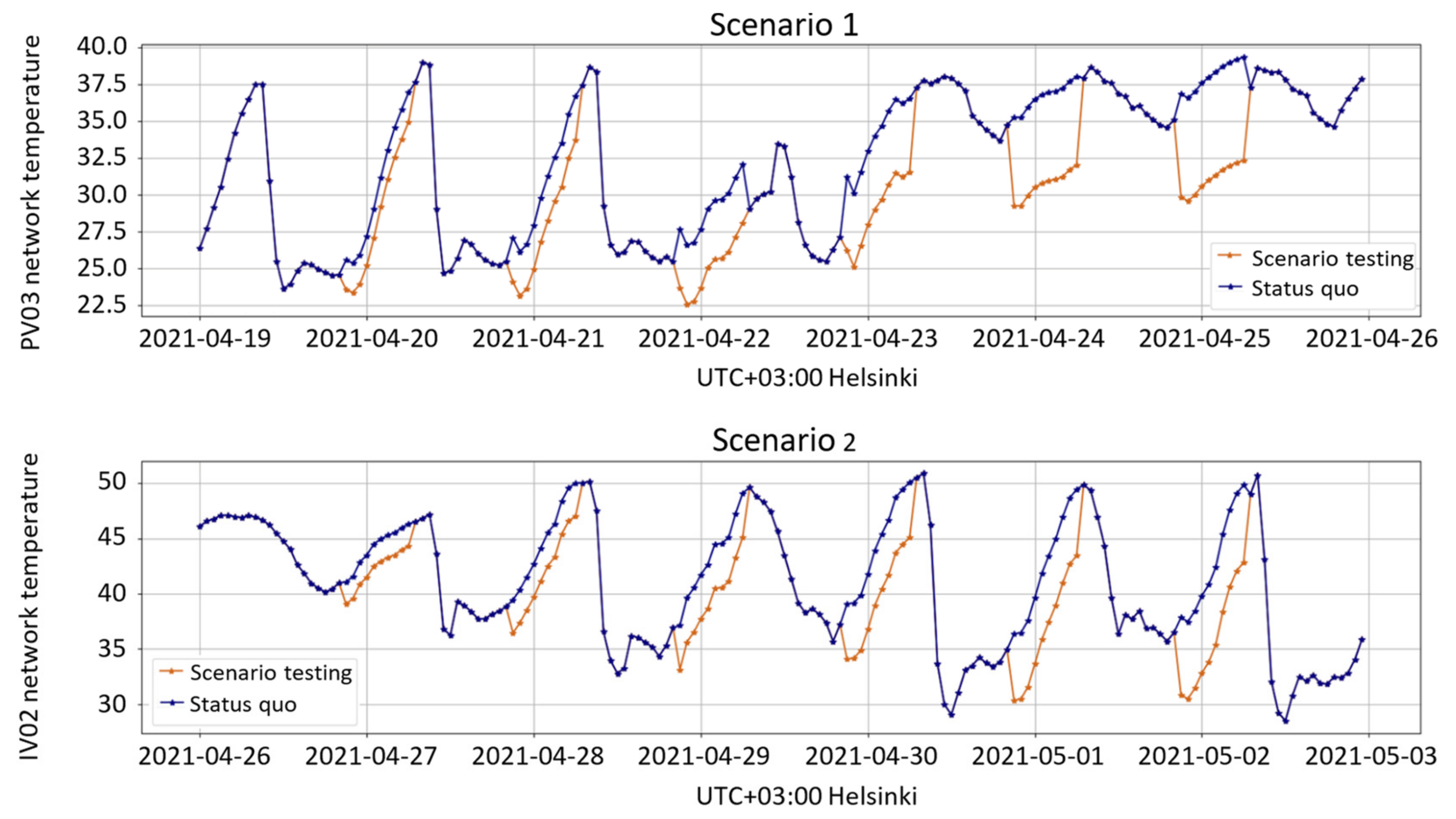
During a 2 week period, more specifically from 19 April to 2 May, scenario testing was conducted in the pilot location in the spring of 2021. These tests included constant decreases to the heating network temperature setpoints in the nights when the location was not in use. The testing was conducted to increase knowledge of the sensitivity of the location’s indoor air quality and the possibilities for energy savings. Additionally, exposing the HVAC system to control schemas outside of the regular operational environment increased the quality of the data.

Table 4. Scenario testing schedule for radiator network.

Week 16	Mon. 9:00 p.m.	Tue. 6:00 a.m.	Tue. 9:00 p.m.	Wed. 6:00 a.m.	Wed. 9:00 p.m.	Thu. 6:00 a.m.	Thu. 9:00 p.m.	Fri. 6:00 a.m.	Fri. 9:00 p.m.	Sat. 6:00 a.m.	Sat. 9:00 p.m.	Sun. 6:00 a.m.
Radiator network	−2	0	−3	0	−4	0	−5	0	−6	0	−6	0
Ventilation network	0	0	0	0	0	0	0	0	0	0	0	0

and

Table 5. Scenario testing schedule for ventilation network.

Week 16	Mon. 9:00 p.m.	Tue. 6:00 a.m.	Tue. 9:00 p.m.	Wed. 6:00 a.m.	Wed. 9:00 p.m.	Thu. 6:00 a.m.	Thu. 9:00 p.m.	Fri. 6:00 a.m.	Fri. 9:00 p.m.	Sat. 6:00 a.m.	Sat. 9:00 p.m.	Sun. 6:00 a.m.
Radiator network	0	0	0	0	0	0	0	0	0	0	0	0
Ventilation network	−2	0	−3	0	−4	0	−5	0	−7	0	−7	0

illustrate the amount of shift in the network control curves as a function of the dates and times of day. During the first week of testing (Week 16 of 2021), the setpoint values of control were decreased for the radiator network from 9:00 p.m. to 6:00 a.m. During the second week of testing (Week 17 of 2021), the ventilation network values were adjusted. Only one heating network out of two in parallel was adjusted during the testing due to the unequal distribution of instrumentation in the building and a careful approach to introducing disturbances to the HVAC system.

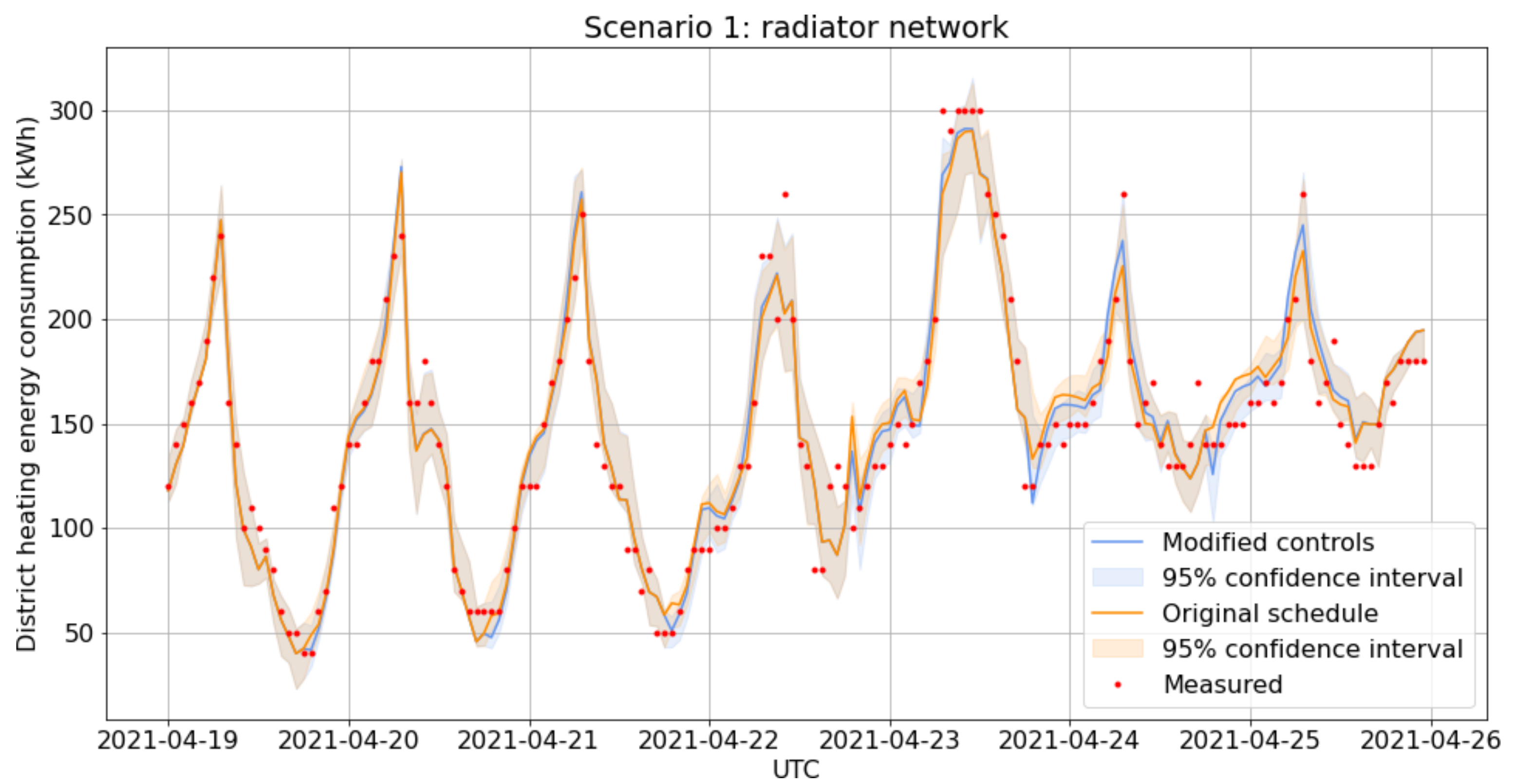
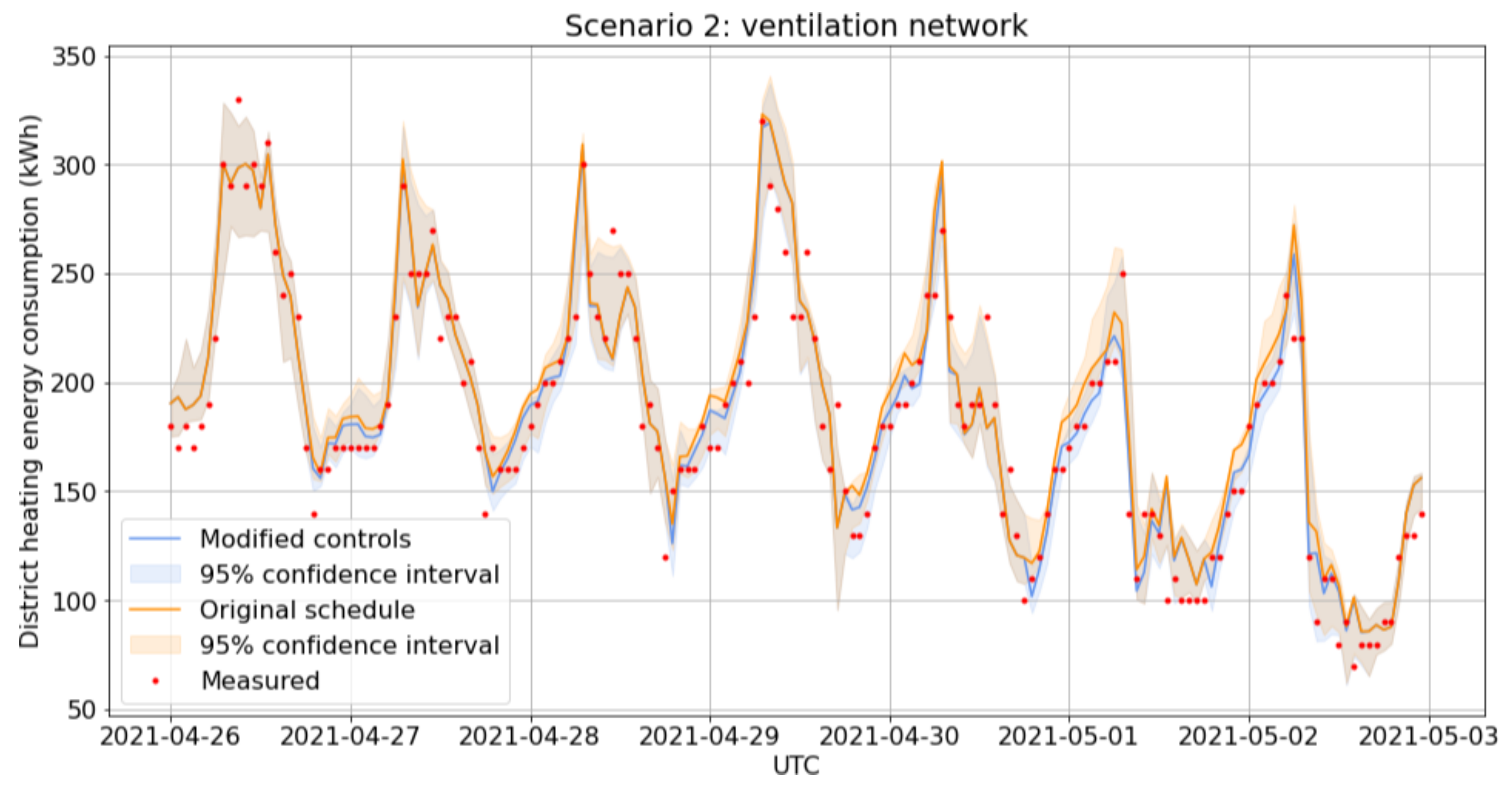
The 10 h adjustments made to network control setpoints resulted in changes to the measurements, as illustrated in Figure 7, where the original controls are shown by the blue line, and the changed measured values are shown in orange.

For scenario testing predictions, the GRU12 model was retrained using the full training data. To reduce the risk of convergence problems, retraining consisted of five independent training runs on the same data, and the model with the smallest testing loss was returned. Energy consumption using the original setpoints was predicted by subtracting the implemented offsets from the measured network temperatures which were assumed to have a causal relationship to energy consumption. The 95% confidence intervals (CI) were estimated as the minimum and maximum values predicted by 20 model instances, each retrained on a bootstrap resample of the training sequences.

3. Results

In this chapter, results of the study are presented from three viewpoints: model tuning, model testing, and scenario testing.

3.1. Model Tuning

The model tuning algorithm specified in Section 2.3 was run for 15 iterations for each model type in the search space defined in

Table 6. Hyperparameter combinations obtained in model tuning.

Algorithm	Units	Layers	Activation Function	Learning Rate	Number of Trainable Parameters
MLP	100	2	ReLU	0.01	11,801
RNN4	120	1	ReLU	0.01	16,441
RNN8	30	1	ReLU	0.01	1411
RNN12	30	1	tanh	0.01	1411
LSTM4	50	1	tanh	0.1	13,251
LSTM8	50	1	tanh	0.01	13,251
LSTM12	40	1	tanh	0.01	9001
GRU4	80	1	tanh	0.01	23,361
GRU8	100	1	tanh	0.01	35,201
GRU12	110	1	tanh	0.01	42,021

. The hyperparameter combinations extracted from the greatest performing models are presented in Table 6, where the number of parameters is included for the sake of illustration. Model tuning was performed only for the ML models, as the OLS estimated linear regression model did not contain suitable hyperparameters.

In Table 6, it can be seen that the model tuning algorithm favored a single-layer structure with a learning rate λ of 0.01 for RNN models. Even though the selections made by the model tuning algorithm indicated notable homogeneity, it is notable that the number of units varied from nearly the bottom of the possible range to the absolute top. This is visible in the amount of variation in the model complexity between optimal models of each model type, i.e., the number of trainable parameters. Additionally, the algorithm favoring ReLUs in RNN models suggests that it might be worth sacrificing the computational efficiency provided by GPU training to include ReLUs as possible activation functions for LSTM and GRU models.

3.2. Model Testing

Model testing was performed with leftover testing datasets presented in

Table 7. Numerically presented training and testing errors of hyperparameter-tuned models.

Algorithm	Training MSE ((kWh)2)	Testing MSE ((kWh)2)
LR	1330	4253
MLP	508.5	1981
RNN4	339.8	2175
RNN8	371.1	1983
RNN12	494.2	2262
LSTM4	629.9	2197
LSTM8	310.5	2230
LSTM12	508.3	2285
GRU4	352.6	1829
GRU8	427.8	2328
GRU12	332.6	1669

. Linear regression parameters were estimated with ordinary least squares, and the best-performing ML models for each model type introduced in Section 3.1 were tested without additional training. As shown in Figure 8, the target values for the hourly energy consumption were compared to forecasts made by the models.

As expected, linear regression was, without question, the worst-performing model of the bunch. This seems to indicate that district heating energy consumption of the HVAC system is not a linear phenomenon with respect to these input features.

When it comes to visual assessment of the performance of the ML models, they seemed to capture the seasonality of energy consumption quite well. They did, however, tend to make similar errors in forecasts as seen in Figure 9. The largest values in energy consumption were chronically underestimated, while other spikes were overestimated. However, the magnitude of the mistakes varied between models, constituting the difference in predictive performance between models.

As visually comparing the performance of the models through the time series plot was not sufficient, the regression errors as mean squared errors were visualized, as shown in Figure 9. The juxtaposition of training and testing errors allowed rough estimates for overfitting in addition to the evident assessment of the models’ predictive performance.

According to Figure 9, the GRU12 model (GRU model with input sequence length of 12) performed the best in terms of the testing errors. GRU4 was the second best, while, rather surprisingly, the static MLP came third in the testing. Displaying a smaller difference between the training and testing errors and relatively good testing performance, the MLP model raises questions regarding the need for sequential models in this framework. A more detailed numerical examination of the regression errors is provided in Table 7.

3.3. Scenario Testing

Scenario testing in the location was performed as outlined in Section 2.4. The purpose of the testing was to increase knowledge of the sensitivity of the location’s indoor air quality and the possibilities for energy savings. The GRU12 model was retrained on the full training data, resulting in the key performance indicators listed in

Table 8. Key performance indicators of the GRU12 model retrained on the full training data.

Algorithm	Dataset	MSE ((kWh)2)	RMSE (kWh)	Bias (kWh)	MAE (kWh)	MAPE
GRU12	Training	334	18.3	0.00455	13.6	6.95%
	Testing	1602	40.0	0.624	28.2	7.78%

. The mean absolute percentage error (MAPE) was 7% for the training and 8% for the testing dataset. As expected from the MSE loss, bias was negligible at less than 1 kWh. Modeling results are presented in Figure 10 and Figure 11. We can see that the measured energy consumption was very close to the simulations with modified controls. This means that we can predict the energy consumption accurately outside the normal operation range even if the input data for the modeling consists of over 90% normal operation data (testing for both the radiator and the ventilation network was for 1 week out of a total of 11 weeks of data collection). The most important indoor air quality parameter is the temperature, and we can conclude that we did not recognize any changes in the temperature during the test period. This means that the temperature was not at all sensitive regarding the temperature setpoint changes of −6 °C for the radiator network and −7 °C for the ventilation network. Energy saving was estimated using the created energy consumption predication model and comparing the energy consumption between original and modified controls. The results are presented in Figure 12. A daily energy saving of 0% (95% CI [0%, 4%]), not statistically significant, was predicted for the 24 h starting at the last 6 °C reduction in the radiation network temperature, and a 5% (95% CI [2%, 8%]) reduction was likewise predicted for the last 7 °C reduction in the ventilation network temperature. Here, it is important to point out that the temperature reduction was applied only for one radiator network and ventilation network, even though the building has two networks.

4. Discussion

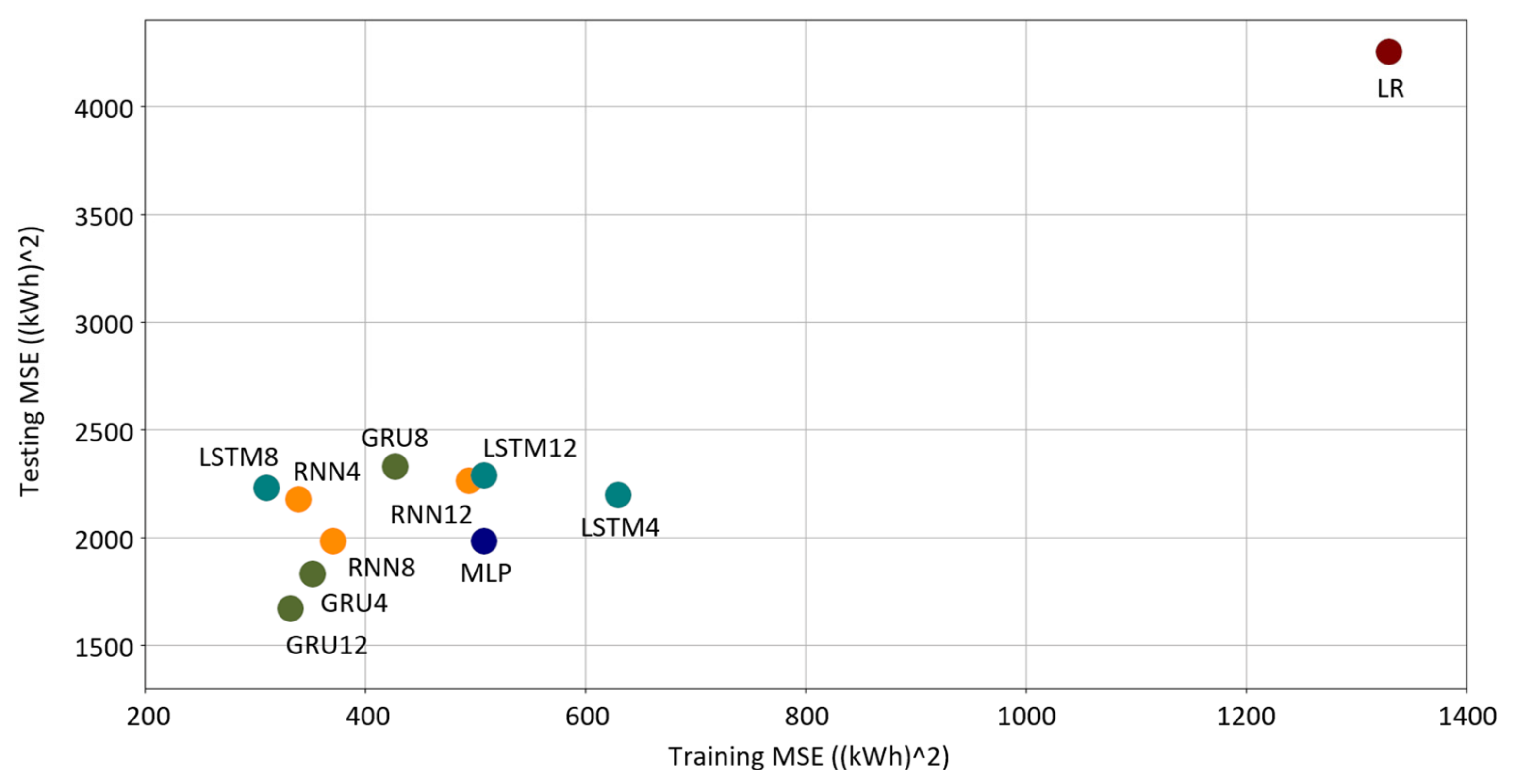
Several ML models were evaluated, and the best-fitting model was selected by applying Bayesian optimization of black-box models to define the ML model’s hyperparameters and by applying a fivefold cross-validation for the assessment of each model’s predictive performance. This presented approach to define the optimum model is in answer to our first research question: What would the optimum ML model structure be for predicting the energy consumption? In this specific case, the optimum ML model was GRU12 (a GRU model with an input sequence length of 12), which performed best in the testing.

Our second research question was as follows: How good are the district heating energy consumption predictions made by ML algorithms for the HVAC system of the pilot location by using normal operational data? Model testing was performed with leftover testing datasets, and the best-fitting model was the abovementioned GRU12. On the other hand, we can conclude that the worst-performing model was LR, which means that the system has nonlinear features; thus, the linear model was not good enough to predict the energy consumption. A GRU12 model was used for two 1 week test periods to predict the energy consumption when the input features were modified from the normal operation range and the prediction results were good. Accordingly, we can state that the developed energy model also has a generalization capability outside the normal operation range where the model was tuned.

In addition to the energy consumption prediction, we can point out that, in our research, we also developed a temperature model to predict the indoor air quality parameter while the available input data were not good enough to predict the temperature, especially outside normal operation range. In fact, our measured indoor air temperature was inside a very narrow band, which obviously poses challenges for modeling the correlation between the features available and the indoor air temperature.

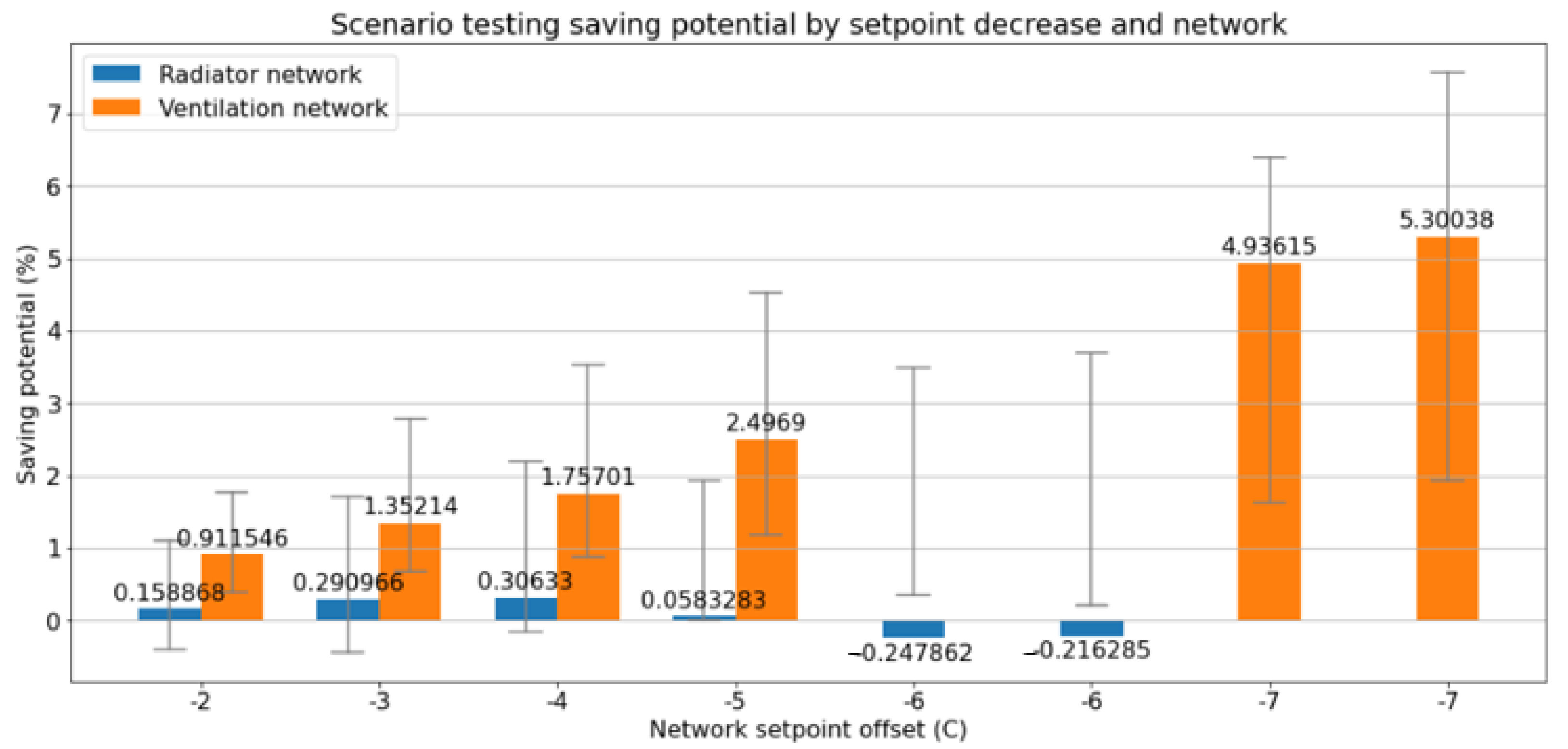
Our third research question was as follows: Can we use the ML model to estimate the energy saving in some scenarios? The 1 week test periods to reduce the water temperature of the radiation networks and the water temperature of the ventilation networks were considered to explore the energy saving potential. This approach to reducing the temperature when buildings are not used (e.g., school buildings are used in the daytime; hence, the temperature could be reduced during the nighttime) is not widely used in practice. Our testing and modeling found a reduction of 5% (95% CI [2%, 8%]) in daily energy consumption by a 7 °C reduction in the ventilation network temperature from 9:00 p.m. to 6:00 a.m., which is quite significant because the temperature reduction was implemented only in after-hours and only in a single ventilation network, even though the building has two radiator and ventilation networks and the energy consumption was for the whole building. This means that there is definitively some possibility to reduce the energy consumption by reducing the ventilation network temperature temporarily, because energy saving can be achieved immediately, while the indoor air temperature is not sensitive regarding the change. We did not find a statistically significant energy saving from radiator network temperature reduction at the 95% confidence level.

The software for hyperparameter tuning and scenario test modeling is available at https://github.com/hamk-uas/HAMK_Smart_City (accessed on 16 June 2022) under a permissive Apache-2.0 license.

5. Conclusions

A six-phase methodology was presented for data preprocessing, which consisted of down-sampling, integration, encoding of cyclical variables, splitting the data for training and testing, scaling, and sequencing. The ML model development was based on data gathering for a period of 11 weeks, and the data originated from five separate sources. The data gathering was performed in an industrial environment during the normal operation of the building. A 1 week test period for the input features such as water temperature of the radiator networks and ventilation networks was used in order to explore the impact on energy saving. The methodology to select the best-fitting model was presented, and it utilized both Bayesian optimization of black-box models to define the ML model’s hyperparameters and fivefold cross-validation for the assessment of each model’s predictive performance.

There are several companies on the market providing so-called SC aimed at achieving energy savings with their algorithms. Our developed model would be beneficial to them to evaluate the achieved energy saving when comparing the energy consumption with static temperatures regarding external conditions and the SC optimized temperature. The developed software on GitHub can be easily adopted for this purpose. Nevertheless, we want to point out that further studies would be recommended to explore our model’s capability to predict the energy consumption in other buildings beyond our pilot case.

One development area would be real-time optimization, which would mean minimizing the energy consumption while keeping the indoor air temperature within agreed tolerances. For the optimization, it would be necessary to calculate the water temperature of radiator networks and ventilation networks so that this requirement would be continuously fulfilled. This would require a temperature model in addition to the developed energy model; therefore, one important further research area would be to develop a reliable temperature model using input data inside the normal operation range.