NMR-Based Study of the Pore Types’ Contribution to the Elastic Response of the Reservoir Rock

Abstract

Seismic data and nuclear magnetic resonance (NMR) data are two of the highly trustable kinds of information in hydrocarbon reservoir engineering. Reservoir fluids influence the elastic wave velocity and also determine the NMR response of the reservoir. The current study investigates different pore types, i.e., micro, meso, and macropores’ contribution to the elastic wave velocity using the laboratory NMR and elastic experiments on coal core samples under different fluid saturations. Once a meaningful relationship was observed in the lab, the idea was applied in the field scale and the NMR transverse relaxation time (T₂) curves were synthesized artificially. This task was done by dividing the area under the T₂ curve into eight porosity bins and estimating each bin’s value from the seismic attributes using neural networks (NN). Moreover, the functionality of two statistical ensembles, i.e., Bag and LSBoost, was investigated as an alternative tool to conventional estimation techniques of the petrophysical characteristics; and the results were compared with those from a deep learning network. Herein, NMR permeability was used as the estimation target and porosity was used as a benchmark to assess the reliability of the models. The final results indicated that by using the incremental porosity under the T₂ curve, this curve could be synthesized using the seismic attributes. The results also proved the functionality of the selected statistical ensembles as reliable tools in the petrophysical characterization of the hydrocarbon reservoirs.

1. Introduction

Nuclear magnetic resonance as a characterization technique of rock media is one of the best techniques to evaluate the presence, quality, and specifications of the fluids in different geological settings. While the conventional logging methods [1,2,3] strongly suffer from the interferences of the inevitable lithological variations, NMR logging simply acts based on the fluids within the pores. This property brings many superiorities to NMR when compared to other logging techniques which are deeply discussed in the published [4,5,6,7,8,9,10,11]. Moreover, despite the complexity of multiple-porosity systems, NMR has shown the capability of producing high-resolution information in these media. On the other hand, nowadays petroleum exploration industry relies on the reflection seismic surveying data as the only tool that could provide the required information of the very deep subsurface formations with a reliable degree of accuracy [12,13,14,15]. From such a point of view, NMR data and seismic data, are considered two of the most precise techniques of exploring hydrocarbon-bearing formations [16,17]. Nevertheless, both these techniques come up with high technical requirements and the subsequent costs are their primary bottleneck. Hence, once these two kinds of data are recorded, researchers and engineers implement various approached to obtain the most possible amount of information hidden within them. Herein, a notable research direction has been employing artificial intelligence techniques to obtain various information on reservoir properties from either kind of the above-mentioned data. These studies have investigated obtaining permeability and porosity from NMR and conventional logs [8,10,18,19,20,21] or estimating petrophysical characteristics from the combination of seismic attributes and well-log data [22,23,24,25]. Meanwhile, novel types of neural networks and deep learning have been introduced for feature engineering of geological data [26,27,28,29].

Considering that the seismic data are recorded in almost all hydrocarbon explorations projects, this research investigates the feasibility of employing seismic data for estimating the NMR bin porosities and then synthesizing NMR T₂ relaxation curves. A bin refers to a subsection of the area under the T₂ curve whilst the entire area represents the overall porosity of the sample. This porosity could also be estimated from the elastic response of the sample in the lab or the equivalent seismic response in the field-scale. Considering that NMR enables us to distinguish between various pore types, i.e., micro, meso, and macropores, in the present study, we carried out elastic and NMR measurements on the same samples in the lab and investigated the contribution of each pore type to the velocity of the compressional wave. We also observed how the fluid saturation affects the elastic and NMR response of an individual core sample and determined the relationship between the changes of the T₂ curve and compressional P-wave velocity under decreasing water saturation. Based on these observations, we then used the intelligent networks to estimate the incremental NMR porosity values from seismic attributes and synthesized the NMR curves in the field scale. To the authors’ best knowledge, neither the relationship between the elastic and NMR response under the effect of fluid saturation nor the introduced method of synthesizing the NMR T₂ curves have not been reported in the existing literature. In the next step, we explored the functionality of statistical ensembles for determining the petrophysical properties of the reservoir and compared their performance with that of the deep learning neural networks. We focused on Bag and LSBoost ensembles. We believe they are also a suitable tool for petrophysical estimations and are equally efficient and in handy as neural networks. The performance of these two ensembles was assessed by estimating NMR permeability values. Throughout the modeling procedure, porosity was adopted as a benchmark to confirm reliability. The studied statistical ensembles proved to be of similar strength as the deep learning network.

Reservoir fluids are the shared link between the elastic and NMR responses of the reservoir rock. Fluid properties such as type, saturation, and density considerably affect both these properties. The existing studies have already proved that the pore fluids have a significant effect on the acoustic impedance and the Poisson’s ratio which is directly correlated with seismic amplitudes [30]. These studies have also verified that the permeability of the reservoir is directly related to its seismic response. A comprehensive discussion on how permeability affects the seismic response and also using seismic attribute analysis for mapping lateral permeability variations of the reservoir can be found in [31,32]. Meanwhile, many studies have determined the relationship between the elastic properties, confining pressure, saturation, and microstructure of the coal and non-coal rocks [33,34,35,36,37,38,39,40]. Even though all these studies highlight that the fluids impact the acoustic and NMR measurements, no study has deeply investigated the relationship between these two different impacts in the laboratory. Meanwhile, even though many researchers have tried to predict various NMR logs from the well-logging data, no study has used the seismic data to estimate the incremental porosity under the T₂ curve and synthesize artificial T₂ distribution curves.

2. Laboratory Experiments of Elastic and NMR Response

2.1. Core Samples

The studied reservoir was the Qinnan coal reservoir located at the southern Qinshui Basin in northern China. The methane-bearing formations of this reservoir are of Carboniferous and Permian ages. The structure of the coal seam in the study area is simple and the coal seam thickness is rather stable with a high gas content. Figure 1 represents the locations of the wells in the studied field.

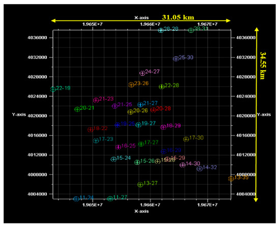
Figure 1. The drilled wells in the coalbed methane (CBM) gas field from where the seismic data and core samples were retrieved.

2.2. Relationship between the Elastic and NMR Responses

Two core samples extracted from the study area were prepared in the laboratory and the elastic wave velocity and NMR T₂ relaxation curves were measured at different degrees of water saturation. First of all, the samples were dried in the oven for 72 h at 80 °C, and then saturated in a vacuum saturation tank. After the full saturation of the samples was achieved, the compressional wave velocity (Vp), as well as the NMR transverse relaxation (T₂) curves, were measured. Next, it was time to desaturate the samples and conducts these two tests again. The desaturation was conducted using centrifuging technique. The measurements were conducted on the samples at three different states, i.e., fully saturated, partially saturated, and irreducible saturation states. For getting the partially saturated state, the two samples were centrifuged at 2000 rpm (revolution per minute) for 45 min, and then the measurements were conducted. Considering that the NMR machine applies a rather high temperature on the samples, we first conducted the elastic experiments and then carried out the NMR tests. After the first set of measurements, the samples were not put back into the centrifuge machine as it was not certain how was the fluid situation inside the pore space after all the procedures applied to the samples. Therefore, the samples were moved back to the saturation tank and were pressurized for two days. Then, the second round of centrifugation was carried out which lasted for 90 min under 3000 rpm. To prevent the breaking of coal samples’ weak skeleton under the centrifuge force, a low revolution speed was applied and the experiment time was increased in order to get to the irreducible fluid saturation. After 1.5 h at this stage, no significant change was observed in the samples’ weight and NMR relaxation curves. This implied that the water in the meso and macropores had been removed from the pore space. Finally, the third set of measurements was conducted. It is worth noting that the elastic wave velocity and T₂ relaxation curves were obtained respectively under the room temperature (24–25 °C) and 32 °C. The relaxation phenomenon was monitored using the CPMG (Carr Purcell Meiboom Gill) pulse sequence where the waiting time was 10 s, inter-echo spacing time was 0.3 ms, the number of scans was 64, and the number of peaks was set to 10,000 on the NMR machine. The results of these experiments are shown in Figure 2. It is worth noting that in this figure, the number of points on the relaxation curve is 100. The inversion algorithm for transforming the free induction decay (FID) to the T₂ relaxation curve was the simultaneous iterative reconstruction technique (SIRT).

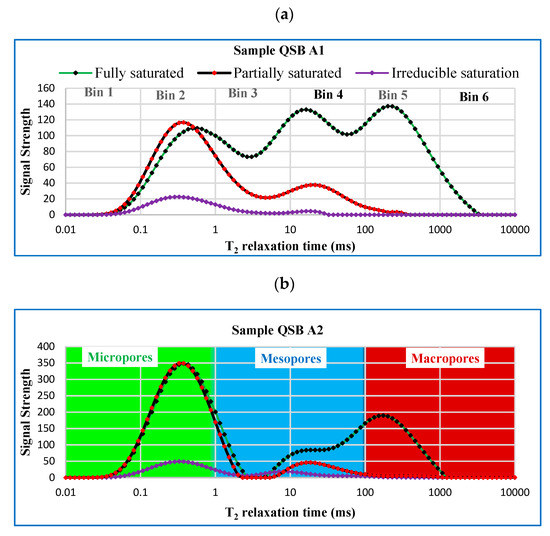
Figure 2. Nuclear magnetic resonance (NMR) T₂ relaxation curves obtained in the laboratory for Sample QSB A1 (a), and Sample QSB A2 (b) under the three states of water saturation, i.e., fully saturated, partially saturated, and irreducible saturation.

While inverting the FID data, the matrix-vector form of the ill-posed inverse Laplace transform problem could be written as:

M = Ea

where M is the measured decay amplitude of size m × 1, E indicates the kernel matrix with the size of m × n, and a is the T₂ spectrum with the size of n × 1. m and n are the numbers of echo trains and predefined T₂ value, respectively. SIRT algorithm is an optimization technique and functions on the premise of algebraic reconstruction. It begins with a simple back-projection, after which the reconstruction is improved iteratively starting from the layergram [41]. The matrix-vector form of the update equation is derived by:

$$a^{t+1}=a^t+CE{E}_q^{T}R\left(m-E_q{a}^t\right)$$

where t represents the steps, $E_q$ is the compressed kernel matrix, and C and R are diagonal matrices that contain the inverse of the sum of the columns and rows of the system matrix represented by:

$$C\left(j,j\right)=\frac{1}{{{\displaystyle \sum }}_{i=1}^m{E}_q\left(i,j\right)} \left(j=1,2,\dots ,n\right)$$

$$R\left(i,i\right)=\frac{1}{{{\displaystyle \sum }}_{j=1}^n{E}_q\left(i,j\right)} \left(i=1,2,\dots ,m\right)$$

More details on this subject could be found in (Ge. et al., 2017) [42].

The area under the NMR curve was divided into six subsections called ‘bins’. The idea is obtained from the Schlumberger CMR tool which divided the T₂ curve into eight bins called CBP (CMR Bin Porosity) and reports the porosity of each bin separately. Bin porosity is equal to the area under one piece of the relaxation curve. The bin porosity of the two samples and the elastic velocities were measured as provided in Table 1. Considering that relaxation occurs faster in smaller pores, they appear at short T₂ times. Hence, the peaks from smaller to larger times respectively represent smaller to larger pores. A peak represents a group of pores with similar sizes. On our test results, we observed three peaks indicating the presence of micropores (x < 2 nm), mesopores (2 < x < 50 nm), and macropores (x > 50 nm) where x indicates the pore size. It is worth mentioning that the microfractures were classified as macropores as well.

Table 1. The results of the laboratory measurements of the elastic and magnetic resonance responses of the coal samples at three states of fully saturated, partially saturated, and irreducible saturation.

	Sample QSB A1			Sample QSB A2
	Fully Saturated	Partially Saturated	Irreducible Saturation	Fully Saturated	Partially Saturated	Irreducible Saturation
Bin 1	54.83	59.04	17.76	216.22	220.74	34.31
Bin 2	1407.12	1550.77	305.33	4518.45	4534.76	637.77
Bin 3	1520.36	610.10	81.81	934.53	555.25	221.21
Bin 4	1877.52	462.29	29.38	1569.87	516.82	135.66
Bin 5	1919.41	49.09	0.00	2290.21	88.20	19.95
Bin 6	214.95	0.00	0.00	14.12	1.68	0.00
VP (m/s)	2813.14	1209.59	1174.65	2735	1430.45	1398.60
Bins summed	6994.19	2731.29	434.28	9543.4	5917.45	1048.9
Decrease in the overall bin area	-	−4262.9	−2297.01	-	−3625.95	−4868.55
Saturation	100%	39%	6%	100%	62%	11%
Decrease in VP (m/s)	-	−1603.55	−34.94	-	−1304.55	−31.85

We observed that the peak of micropores was located in bin 2. Likewise, the peaks of mesopores and macropores respectively appeared in bins 3–4 and bin 5. Therefore, we classified the pore space into three sections of the micropores, mesopores and macropores as shown in Figure 2. Then we analyzed the contribution of each bin and each pore type to the elastic wave velocity as shown in Figure 3 (top).

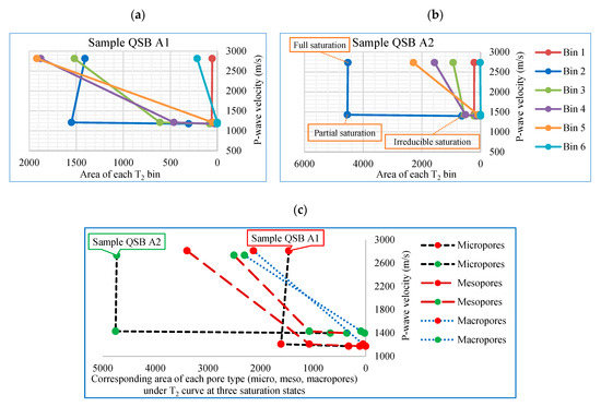
Figure 3. (a,b) Analyzing the contribution of each pore type (micro, meso, and macropores) to the decrease of elastic P-wave velocity for Sample QSB A1 and Sample QSB A2. The three data points on each graph represent the three saturation states, from left to right: full saturation, partial saturation, and irreducible saturation, respectively; (c) The green and red colors indicate the corresponding data points of the two samples. For each sample, there are three curves, which show the changes of microporosity (black dashed line), mesoporosity (dark red long-dashed line), and macroporosity (blue dotted line) of that sample at three saturation states, from left to right: full saturation, partial saturation, and irreducible saturation, respectively. The porosity value for each pore type at each saturation state was calculated by summing the values of bins 1–2 (for microporosity), bins 3–4 (for mesoporosity), and bins 5–6 (for macroporosity).

When centrifuging the samples, the fluid in the larger pores escapes the sample first. This is highlighted by the disappearance of the corresponding peak on the T₂ curve as we observed in the tests as well. When the fluid runs out and larger pores get filled with air, the acoustic velocity drastically decreases. Such a decrease can be seen in Figure 3 (bottom). This phenomenon followed the same trend in each pore type (micro, meso, and macropores) on both samples. Moreover, the rate of decrease (slope of the curve) was the fastest for micropores, then for mesopores, and the slowest for micropores. This is again because of the influence of the pore size on the fluid’s capability to move These observations are in agreement with our fundamental understanding of the NMR and waves’ traveling phenomena within the porous media and verify the reliability of the results. Figure 4 illustrates the two adopted samples and also indicates the various pore types observed in the scanning electron microscopy (SEM) images of the samples. As can be seen, pores of different sizes existed inside the samples and the range of the pore size distribution was rather wide. Meanwhile, the existing pores appeared as pore-clusters with different sizes or as independent pores being dispersed at different locations.

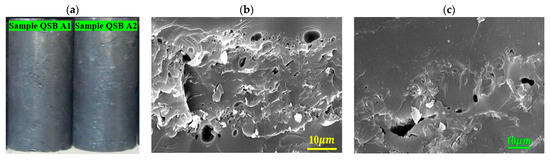
Figure 4. (a) The two studied samples; (b,c) Various pore types, i.e., micro, meso, and macropores inside the Sample QSB A1 and Sample QSB A2, respectively, under the scanning electron microscope. These SEM images only represent the qualitative situation of the internal pore space of the samples and the real bulk porosity was quantitatively measured by the NMR machine.

Figure 5 shows the relationship between the changes in the elastic and NMR responses of the two coal core samples for the cumulative amount of area under the T₂ curve. As follows from this figure, the decreasing saturation causes a decrease in both responses of the core samples. This decrease is fast in higher saturation values (from full to partial saturation) and slows down in the lower saturation values (from partial saturation to irreducible saturation state). This is because, in higher saturations, the fluids considerably stimulate the compressional wave [43,44,45]. Moreover, since the combined amount of meso and macropores were larger for Sample QSB A1 than the Sample QSB A2 (79.02% vs. 50.4%), the decrease was faster in this sample.

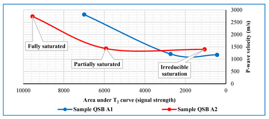
Figure 5. The relationship between the changes in the elastic and NMR responses of the two coal core samples in the laboratory. Three data points from left to right respectively indicate the fully saturated, partially saturated, and irreducible saturation states.

Figure 6 represents the relationship between water saturation with the area under the T₂ curve and P-wave velocity. As expected, and described above, the area under the T₂ curve and P-wave velocity should decrease with the decreasing fluid saturation. We also compared our results with observations of other researchers in the literature [33,43] and found an acceptable agreement.

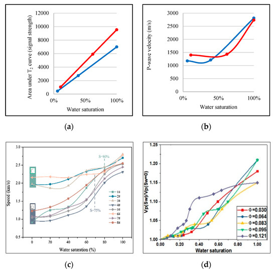
Figure 6. The relationship between water saturation and area under T₂ curve (a), and P-wave velocity (b). Our results were compared with the existing literature: (c) after [33] and (d) after [43].

In our tests, the cut-off values for micro, meso, and macropores were respectively 1, 10, and 100 ms. Finally, we could calculate the contribution of each pore type to the elastic wave velocity using the following relationships. These relationships are for full saturation status. In well logging practices, Wyllie’s time equation is generally used to define the relationship between the porosity and sonic transit time as [46,47,48,49]:

$$\Delta t=\Delta t_{ma}\left(1-{\varphi }_s\right)+\Delta t_f{\varphi }_s$$

(1)

$${\varphi }_s=\frac{\Delta t-\Delta t_{ma}}{\Delta t_f-\Delta t_{ma}}$$

(2)

where $\Delta t$, $\Delta t_{ma}$, and $\Delta t_f$, all in $\left(\mathsf{\mu }\mathrm{s}/\mathrm{ft}\right)$ respectively indicate is the transit time of elastic wave in the rock sample, the transit time of the matrix, and the transit time of the fluid. Moreover, ${\varphi }_s$ is the porosity derived from sonic measurements.

Since the porosity of each pore type could be calculated as:

$${\varphi }_{mic}={\varphi }_s\frac{{{\displaystyle \int }}_{T_2=0.01}^{T_2=1}{T}_{2}dt}{{{\displaystyle \int }}_{T_2=0.01}^{T_2=10000}{T}_{2}dt}$$

(3)

$${\varphi }_{mes}={\varphi }_s\frac{{{\displaystyle \int }}_{T_2=1}^{T_2=100}{T}_{2}dt}{{{\displaystyle \int }}_{T_2=0.01}^{T_2=10000}{T}_{2}dt}$$

(4)

$${\varphi }_{mac}={\varphi }_s\frac{{{\displaystyle \int }}_{T_2=100}^{T_2=10000}{T}_{2}dt}{{{\displaystyle \int }}_{T_2=0.01}^{T_2=10000}{T}_{2}dt}$$

(5)

By using the above-described incremental area under the T₂ curve., we could finally determine the contribution of each pore type to the elastic wave’s transit time as:

$$\Delta t_{mic}={\varphi }_{mic}\left(\Delta t_f-\Delta t_{ma}\right)+\Delta t_{ma}$$

(6)

$$\Delta t_{mes}={\varphi }_{mes}\left(\Delta t_f-\Delta t_{ma}\right)+\Delta t_{ma}$$

(7)

$$\Delta t_{mac}={\varphi }_{mac}\left(\Delta t_f-\Delta t_{ma}\right)+\Delta t_{ma}$$

(8)

According to the NMR results, micro, meso, and macropores respectively contributed to 21%, 48.5%, and 30.5% of the total porosity of the Sample QSB A1 and to the 49.6%, 26.2%, 24.1% of the total porosity of the Sample QSB A2, respectively. The overall porosities of these two samples were respectively 4.3% and 5.6%. This implies that the micro, meso, and macro porosities of the samples were respectively 0.9%, 2.09%, 1.31% for Sample QSB A1 and 2.78%, 1.47%, and 1.35% for Sample QSB A2. Considering that different pore types occupied dissimilar portions of the pore space in the two samples, their impact on the elastic wave velocity was also different. The length of the samples was 5 cm, so the overall transit times in the two samples were respectively 17.8 μs and 18.3 μs, for which respectively 0.76 μs and 1.03 μs referred to the pore space. Herein, contributions of the mico, meso, and macropores to the transit time of the elastic wave in Sample QSB A1 were respectively 0.16, 0.37, 0.23 μs, and in Sample QSB A2 were respectively 0.51, 0.27, 0.25 μs. It is worth noting that these values represent the average value as the wave propagation inside the pore space happens simultaneously in all pore types.

3. Field-Scale Estimation of Relaxation Curves

3.1. Seismic and NMR Data from the Field

After the impact of the fluid saturation, as well as the contribution of micro, meso, and macropores to the overall transit time of the elastic wave, were determined, the idea was used to estimate NMR bin porosities from the seismic attributes and synthesize artificial T₂ relaxation curves. This stage of the study started by selecting the NMR well-logging data and the seismic data cube. The data was preprocessed and the seismic attributes at the well locations were extracted. These attributes were calculated as described in Table 2.

Table 2. A brief explanation of the most important seismic attributes employed in the current study [50].

Instantaneous Frequency	Instantaneous frequency is the time derivative of the phase. This attribute should not be confused with the frequency of the wavelet. It is often used to estimate seismic attenuation. Oil and gas reservoirs usually cause drop-off of high-frequency components. It helps to measure cyclicity of geological intervals and can be useful for cross-correlation across faults. It could also identify contacts between gas and water or gas and oil. Instantaneous frequency tends to be unstable in the presence of noise and is sometimes difficult to interpret. This attribute is calculated as: $\mathsf{\omega }=\frac{\mathsf{\delta }\mathsf{\theta }}{\mathsf{\delta }\mathrm{t}}$
Instantaneous Phase	The attribute is calculated on a sample by sample basis without regard of the waveform. The attribute provides an amplitude independent display. It is commonly used to find continuity of weak events and to distinguish small faults and dipping events. Instantaneous phase is calculated as: $\mathsf{\theta }=ta{n}^{-1}\left(\frac{g}{f}\right)$
Frequency Filter	The frequency-filter attribute is useful for enhancing particular seismic events or to reduce unwanted noise in the data. This can improve the accuracy of interpretation.
Apparent Polarity	The polarity of the instantaneous phase, calculated at the local amplitude extreme. The apparent polarity reveals the sign of the reflection coefficient and therefore indicates features that would change it, e.g., unconformities. It is useful for checking the lateral variation of polarity along a reflection layer. On a noisy seismic section, event continuity can be clearer on the apparent polarity than the original seismic section. This attribute reveals reflection details without the waveform effects and can help detect thick beds when the data is of good quality (less noise).
Amplitude Envelope	The total instantaneous energy of the analytic signal (the complex trace), independent of phase, calculated as: $\sqrt{f^2+g^2}$ where f and g are the “real” and “imaginary” components of the seismic trace. So, if f is the real part, which are just the original seismic trace samples, g will be the samples from the Hilbert transform (also called quadrature amplitude) of the seismic trace.
Relative Acoustic Impedance	Relative acoustic impedance is a running sum of regularly sampled amplitude values. This attribute is calculated by integrating the seismic trace and passing the result through a high-pass Butterworth filter with a hard-coded cut-off at (10*sample rate) Hz.
Reflection Intensity	Reflection Intensity is the average amplitude over a specified window (9 samples in the present study) multiplied with the sample interval. Reflection Intensity is useful for the delineation of amplitude features while retaining the frequency appearance of the original seismic data.
RMS Amplitude	RMS amplitude is the square root of the sum of the squared amplitudes divided by the number of live samples as shown in the following formula: $\sqrt{\frac{\left({{\displaystyle \sum }}_i^{n}am{p}^2\right)}{K}}$
Second Derivative	The second time derivative of the input seismic volume. The combination of the original amplitude, first derivative, and second derivative allows you to express seismic interpretation in relationship to maximum, minimums, greatest descents, and descent polarity. The second derivative can be used to help guide the pick by providing continuity in areas of where reflections are poorly resolved on the raw amplitude. Lateral amplitude variations are visibly diminished, which will make auto-tracking regional events more difficult.

The intelligent models learned to predict CMR bin porosities from the seismic attributes. In the study area, the NMR data was presented by eight bin values, namely CBP1-CBP8. The three most significant components of a seismic trace include its amplitude, frequency, and phase. Therefore, in order to have robust models, the input attributes of the neural network models should include a representative of every property (Figure 7). Eventually, five attributes from among more than 13 seismic attributes including seismic inversion results, integrate of the amplitude values, two-way-time (TWT), derivative instantaneous amplitude, squared inversion, amplitude weighted cosine phase, frequency filter, cosine instantaneous phase, instantaneous frequency, amplitude weighted phase, integrated absolute amplitude, and inverted inversion (inversion⁻¹) etc. were selected as the input elements of the modeling task. These attributes were chosen based on the researchers’ knowledge of the study area and also the analysis of cross-correlation values. Alongside the seismic section, Figure 8 illustrates four examples of these attributes at the location of one studied well. Table 3 shows the linear relationship of the inputs and targets of our modeling process that were CBPs and each of the input attributes. It is worth mentioning that for successful modeling using the intelligent estimators, there should be a meaningful relationship between the input and target values, implying that irregular distributions of data on a crossplot would not lead to reliable results. The stronger this relationship is, the better the modeling results would be. While the liner relationship is the simplest form, the neural networks use high-order polynomial relationships, for which the cross-correlation values are much larger than the linear manner.

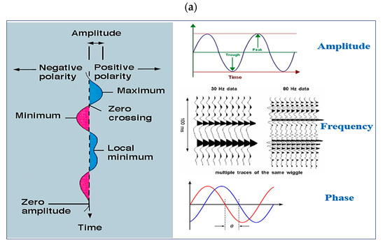
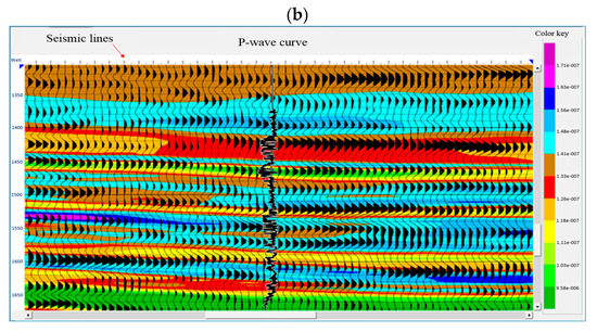
Figure 7. (a) The most significant components of a seismic trace; (b) Raw seismic data (Wiggle traces) and acoustic impedance inversion (color attribute) in the location of one of the studied wells overlain by the P-wave velocity from logging curve.

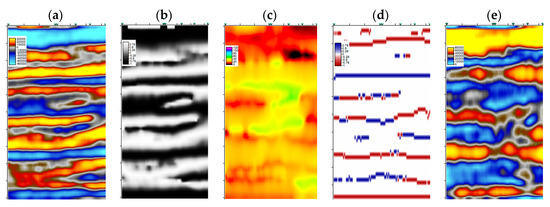
Figure 8. Two-dimensional (2D) seismic section passing through the employed well (a); and its four corresponding seismic attributes, including cosine of phase (b), instantaneous frequency (c), apparent polarity (d), and amplitude envelope (e).

Table 3. Linear relationships of the seismic attributes (inputs) and CBPs (outputs)

CBP1	Attribute	R2	CBP2	Attribute	R2
	Derivative Instantaneous Amplitude	0.1315		Inversion	0.1236
	Squared Inverted Inversion	0.1320		Derivative Instantaneous Amplitude	0.1070
	TWT	0.1586		Frequency Filter	0.1650
	Frequency Filter	0.2018		Instantaneous Phase	0.1112
	Amplitude Weighted Cosine Phase	0.1341		TWT	0.1446
CBP3	Squared Inversion	0.2728	CBP4	Amplitude Weighted Cosine Phase	0.2302
	Cosine Instantaneous Phase	0.3860		Instantaneous Frequency	0.2745
	Seismic Amplitudes	0.4238		Frequency Filter	0.4918
	Amplitude Weighted Cosine Phase	0.3140		Cosine Instantaneous Phase	0.5503
	Amplitude Integrate	0.3130		Seismic Amplitudes	0.6225
CBP5	Amplitude Weighted Cosine Phase	0.3602	CBP6	Instantaneous Frequency	0.4461
	TWT	0.3655		Frequency Filter	0.5483
	Squared Inversion	0.4747		Amplitude Weighted Phase	0.4575
	Cosine Instantaneous Phase	0.5098		Cosine Instantaneous Phase	0.4182
	Seismic Amplitudes	0.5747		Seismic Amplitudes	0.4654
CBP7	Derivative Instantaneous Amplitude	0.4885	CBP8	Amplitude Weighted Cosine Phase	0.3428
	Inverted Inversion	0.7804		Derivative Instantaneous Amplitude	0.3969
	Amplitude Integrate	0.6728		Inverted Inversion	0.7129
	Amplitude Weighted Cosine Phase	0.4530		TWT	0.5693
	TWT	0.7173		Integrated Absolute Amplitude	0.1402

3.2. Estimating NMR CBPs from Seismic Attributes

After providing the input seismic attributes and CMR data, the next step was defining the intelligent models. Herein, we used neural networks and fuzzy logic models. In order to have a more reliable estimation, several different neural network algorithms were adopted and the best-performing one was selected as the final estimator. This model produced the smallest error and the best correlation. The input arguments of the constructed models were seismic attributes and the outputs were CBP values of the T₂ curves. Herein, the backpropagation neural networks (BP-NN) were adopted. BP-NN is a type of supervised-training network. We made use of feedforward BP-NN with 20 or 40 neurons in their hidden layers. The tangent sigmoid (TANSIG) function was used to introduce nonlinearity to the system. These backpropagation neural networks were trained respectively by Levenberg–Marquardt (LM), resilient back-propagation (RP), one step secant (OSS), scaled conjugate gradient (SCG), Conjugate Gradient with Powell/Beale Restarts (CGB), and back-propagation with adaptive learning rate (GDA). Finally, the network with the best performance was selected as the final intelligent model for estimating each CBP value. The performance was determined using the mean square error (MSE) and the determination coefficient (R²).

Table 4 represents the number of data points used either for constructing or for testing the accuracy of the final estimators. This means that we selected about 80% of our data for making the models and used the other 20%, which was unforeseen by the models during their construction, to test the models’ accuracy and prove their reliability. It is worth mentioning that for each of the employed algorithms, an adequately large number of models were developed. Since fuzzy logic and ANFIS (hybrid neuro-fuzzy) models did not perform as well as neural networks, the results are not represented.

Table 4. Properties of the training data and performance of the intelligent models.

Target Curve	CBP1	CBP2	CBP3	CBP4	CBP5	CBP6	CBP7	CBP8
No. of input attributes	5	5	5	5	5	5	5	5
Total No. of available data pairs	520	277	476	536	545	431	503	568
No. of training and validation data	442	235	405	456	463	366	428	483
No. of test data	78	42	71	80	82	65	75	85
No. of neurons in hidden layers	30	30	30	30	30	30	30	30
Iteration the best ANN model was achieved	321	203	311	260	288	346	198	169
Performance of the ANN model (MSE)	1.12 × 10−5	2.27 × 10−5	1.05 × 10−5	1.80 × 10−4	8.41 × 10−5	7.06 × 10−6	6.92 × 10−6	2.29 × 10−5
Correlation with measured data (R2)	0.93	0.81	0.88	0.99	0.98	0.94	0.98	0.94

As mentioned earlier, the ANN models varied in the number of their internal neurons and their training algorithms. Each ANN model was retrained for 400 times and the optimal model was selected. The iteration at which the optimal was achieved is outlined in Table 4. Additionally, to guarantee the comprehensiveness of the developed estimators, the training and test data sets were chosen in a way that would track the trend of geological variations reflected in the NMR T₂ relaxation curves. Concerning the neural network modeling tasks, the training algorithm is the most crucial factor that would influence the quality of the prediction task. On account of this fact, in this research, we used six independent training algorithms and observed their estimation capability. This comparison is represented in Table 5, Table 6, Table 7 and Table 8. These tables show the agreement of estimated CBP values with the measured ones.

Table 5. Comparison between the performance of various ANN training algorithms for bins 1 and 2.

	Modeled Parameter	CBP1		CBP2
Training Algorithm		R2	MSE	R2	MSE
conjugate gradient with Powell/Beale restarts (CGB)		0.73	7.19 × 10−5	0.67	6.95 × 10−5
back-propagation with adaptive learning rate (GDA)		0.67	9.49 × 10−5	0.66	5.32 × 10−5
Levenberg–Marquardt (LM)		0.93	1.12 × 10−5	0.81	2.27 × 10−5
one step secant (OSS)		0.63	1.35 × 10−4	0.71	1.70 × 10−5
resilient back-propagation (RP)		0.62	9.21 × 10−5	0.66	3.43 × 10−5
scaled conjugate gradient (SCG)		0.76	4.65 × 10−5	0.69	3.12 × 10−5

Table 6. Comparison between the performance of various ANN training algorithms for bins 3 and 4.

	Modeled Parameter	CBP3		CBP4
Training Algorithm		R2	MSE	R2	MSE
conjugate gradient with Powell/Beale restarts (CGB)		0.78	2.60 × 10−5	0.94	1.60 × 10−3
back-propagation with adaptive learning rate (GDA)		0.71	1.52 × 10−5	0.87	3.20 × 10−3
Levenberg–Marquardt (LM)		0.88	1.05 × 10−5	0.99	2.00 × 10−4
one step secant (OSS)		0.79	2.64 × 10−5	0.92	1.20 × 10−3
resilient back-propagation (RP)		0.76	3.02 × 10−5	0.88	3.00 × 10−3
scaled conjugate gradient (SCG)		0.83	3.66 × 10−5	0.94	1.50 × 10−3

Table 7. Comparison between the performance of various ANN training algorithms for bins 5 and 6.

	Modeled Parameter	CBP5		CBP6
Training Algorithm		R2	MSE	R2	MSE
conjugate gradient with Powell/Beale restarts (CGB)		0.94	2.93 × 10−4	0.91	1.12 × 10−5
back-propagation with adaptive learning rate (GDA)		0.93	2.85 × 10−4	0.83	3.17 × 10−5
Levenberg–Marquardt (LM)		0.98	8.41 × 10−5	0.94	7.06 × 10−5
one step secant (OSS)		0.93	3.14 × 10−4	0.84	2.09 × 10−5
resilient back-propagation (RP)		0.91	3.99 × 10−4	0.88	1.49 × 10−5
scaled conjugate gradient (SCG)		0.92	2.62 × 10−4	0.90	1.39 × 10−5

Table 8. Comparison between the performance of various ANN training algorithms for bins 7 and 8.

	Modeled Parameter	CBP7		CBP8
Training Algorithm		R2	MSE	R2	MSE
conjugate gradient with Powell/Beale restarts (CGB)		0.95	1.54 × 10−5	0.90	4.04 × 10−5
back-propagation with adaptive learning rate (GDA)		0.95	1.49 × 10−5	0.90	4.11 × 10−5
Levenberg–Marquardt (LM)		0.98	6.92 × 10−6	0.94	2.29 × 10−5
one step secant (OSS)		0.94	1.90 × 10−5	0.91	4.14 × 10−5
resilient back-propagation (RP)		0.93	1.95 × 10−5	0.90	4.23 × 10−5
scaled conjugate gradient (SCG)		0.95	1.62 × 10−5	0.92	4.20 × 10−5

According to the obtained results, among the adopted techniques, the Levenberg-Marquardt training algorithm was selected as the best performing model for estimating all CBP values. While for NN models, the training algorithm is the most influencing factor on the quality of the output results, for the fuzzy and neuro-fuzzy models, clustering radius is the most important factor. However, neither fuzzy nor neuro-fuzzy models did not lead to acceptable results. It is worth mentioning that in our study most neural networks came to relatively acceptable results. However, Table 4 only presents the performance of the best models rather than all developed models. After all, CBP2 and CBP3 were predicted weaker than the others. These two bins fall in the category of micropores and the reason for their lower prediction would be the complexity of the magnetization relaxation in smaller pores. Nevertheless, all other bin values were estimated with an accuracy of more than 93%. We believe the most important reason for such a good performance is that the input data comprehensively encompassed different petrophysical features of the geological formations. The cross-correlations of the predicted and measured CBP values are illustrated in Figure 9.

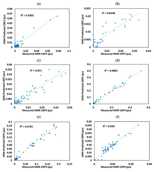
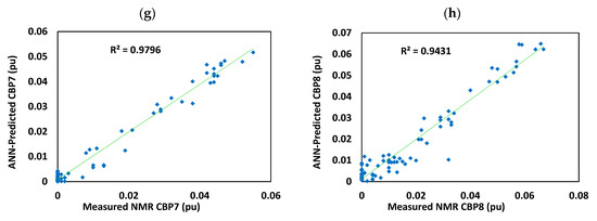
Figure 9. Correlations of the measured values of bin porosities with the predicted values (pu indicates the porosity unit): (a) CBP1; (b) CBP2; (c) CBP3; (d) CBP4; (e) CBP5; (f) CBP6; (g) CBP7; (h) CBP8.

Finally, the T₂ relaxation curves could be synthesized. Figure 10 depicts the comparison between the measured and predicted T₂ curves at ten different depths of the test well. These ten points serve as an example and, based on the established models, the simulation process would be done in any desired section of the well or the area surrounding the well as far as no considerable changes happen in the geological conditions of the objective area compared to the well locations where the models were developed. As can be seen from this figure, models performed satisfyingly in estimating T₂ relaxation curves and successfully draw out the general trend of relaxation variations that can be very useful in case of the quick, inexpensive, and in handy evaluation of the geological formations.

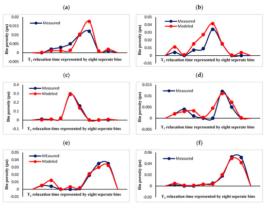
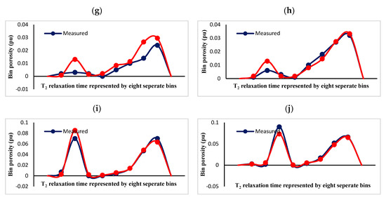
Figure 10. (a–j) Measured and predicted T₂ relaxation curves at ten example points of one studied well. Such relaxation curves could be synthesized for every desired part of the reservoir using the established models and the introduced method.

After we predicted NMR T₂ curves in the location of the studied wells, and since the models proved to be trustworthy, we tried to upscale our prediction model and estimate the T₂ curves for areas around one of the wells in the studied coal formation. Figure 11 illustrates the 3D structure of this formation in the entire coalbed methane field. Figure 12 shows the predicted curves at the corresponding depths of the coal formation, and also illustrates the location of the simulation area and the position of the well around which the models were upscaled. Figure 13 represents the results of the upscaling procedure and shows the simulated NMR T₂ transverse relaxation curves at various depths.

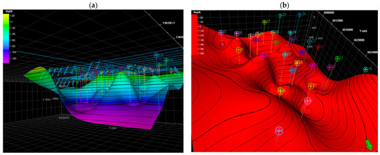
Figure 11. (a,b) The coal formation in the subject CBM gas field from two different views. The thickness of the coal layer is in the range of 2–8.3 m.

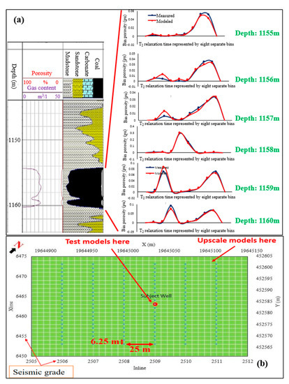
Figure 12. (a) Predicted T₂ curves in the corresponding depths on the well-logging section; (b) Map of the areas and position of the selected simulation nods compared to the subject well. The spacing of the seismic survey inlines and xlines are respectively 25 m and 6.25 m on the map. Therefore, the simulation covered an area of 125 × 125 m² at the depth of 1157 m.

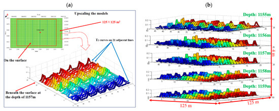
Figure 13. (a) The finally simulated T₂ curves in the depth of 1157 m and their corresponding position on the surface; (b) Simulated T₂ curves at various depths of the reservoir which could be estimated for any desired area around the well as far as no considerable geological changes happen.

4. Statistical Models and Deep Learning

4.1. Bag and LSBoost Ensembles

The present study examined the performance of the statistical Bag and Least Square Boosting (LSBoost) ensembles in predicting the petrophysical properties of the reservoir and compared their performance with those of deep learning regression networks. Statistical ensembles are user-friendly and in handy which could be of great applications in the assessment of the reservoir layers. They also require less memory than intelligent techniques when analyzing large-sized field data.

Statistical supervised learning splits into two broad categories namely classification, and regression [51]. The regression technique is used when the problem involves modeling and analyzing the relationship between a dependent and one or more independent variables. Within the regression category, ensemble learning is a framework of combining multiple weak learning algorithms to produce a strong learning algorithm [52]. The present research utilized regression ensembles, as the statistical supervised learning machines, to obtain permeability and porosity information from 3D seismic attributes. The ensemble algorithms used herein were regression Bag and Least Square Boosting (LSBoost) that were implemented in the MATLAB environment. Bagging and boosting algorithms both learn from weak learners, but Bagging trains weak learners in parallel while boosting trains them in a sequential manner (Figure 14) [53]. The ensembles in this research included decision trees as their weak learners to predict responses to the input data. The selection of the number of trees inside each type of ensemble algorithms was based on the performance analyses of 200 various ensembles. This means that by changing the number of trees in the range of [1–200], numerous Bag and LSBoost ensembles were created and their performance in predicting the new data was observed. The purpose of this step was to obtain the optimal number of weak learners (Figure 15). At the next step, the most reliable ensemble was selected as the optimal model for further usage and predicting permeability or porosity. The method which was used for evaluating this final ensemble’s quality was using an independent test data set (30% of the available well data). It is worth mentioning that Bagging is oriented towards decreasing variance and boosting is oriented towards decreasing bias, and LSBoost is faster in training.

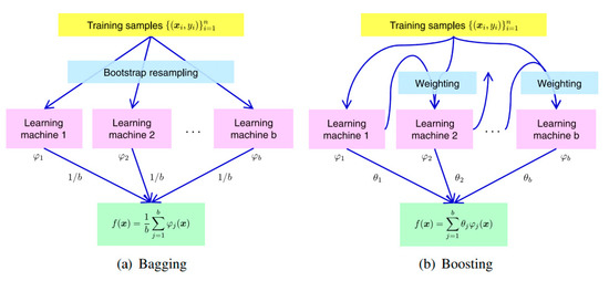
Figure 14. Ensemble learning. Bagging (a) trains weak learners in parallel while boosting (b) trains them sequentially [53].

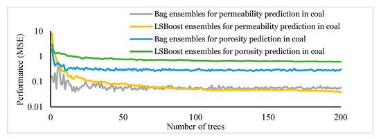
Figure 15. Prediction error versus the number of trees for statistical ensembles in the studied unconventional coal reservoir.

4.2. Deep Learning and Deep Belief Network

Deep learning is rather the latest achievement of artificial intelligence and machine learning that has captured the imagination of countless scientists and researchers. Deep learning refers to the in-depth feature engineering through successive layers of neural networks for increasingly meaningful representations of the data [54]. Deep herein doesn’t mean any kind of deeper understanding of the data, but it rather means the larger number of the functioning layers. A deep learning network consists of an input layer, several hidden layers, and an output layer. Deep architectures would be constructed by stacking autoencoders or by using deep belief networks (DBNs) [55]. DBN is the most effective technique among all deep learning models and is the technique of stacking many individual unsupervised networks that use each network’s hidden layer as the input for the next layer. The DBN implemented in the present study stacked restricted Boltzmann machines (RBM) in the hidden layers. The deep hierarchy of a DBF transforms the input features into nonlinear higher-level abstractions to extract more significant patterns and follow the trends in the input space [56]. These layers are first trained in an unsupervised manner. The structure of our adopted DBN consisted of four hidden layers with the sizes of 200, 100, 50, and 25 nodes, with eight input neurons (seismic attributes) and one output neuron (permeability or porosity). The RBMs were trained with a sigmoid activation function. They would also be trained using rectified linear activation units (ReLU). It is worth noting that in a deep learning network, it is also feasible to keep the size of all hidden layers the same. However, this approach was not implemented in this study. An RBM consists of a visible and a hidden layer where the hidden units are not connected to each other but have undirected, symmetrical connections to the visible units [56]. In other words, every node in the visible layer is connected to every node in the hidden layer, but no nodes in the same group are connected as depicted in Figure 16. The details on RBM could be found in [57,58].

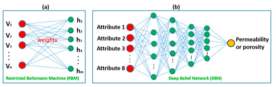
Figure 16. (a) Graphical description of restricted Boltzmann machine (RBM) with n visible and m hidden units; (b) deep belief network (DBN) adopted in the present study with four hidden layers, eight input neurons, and one output neuron.

If the sigmoid activation function is:

$$S\left(y\right)=\frac{1}{1+e^{-y}}$$

(9)

Then, the output of the neuron will be:

$$p\left(S_i=1\right)=\frac{1}{1+\exp \left(-b_i-{{\displaystyle \sum }}_j{S}_i{w}_{ij}\right)}$$

(10)

where $w_{ij}$ is the weight value that the j^th hidden layer assigns to the i^th input value [56].

The selected attributes for developing the statistical and artificial neural network (ANN) models of the reservoir are represented in Table 9, and the seismic cube from which the attributes were extracted is shown in Figure 17. This table also shows the dependence of each target parameter, namely porosity and permeability, on each of the input parameters. For this reservoir, the permeability and porosity models were developed respectively using 231, and 355 data points. Both these parameters were estimated using 8 input attributes. Herein, approximately 70% of the entire data set was employed to train the models. The rest of the available data was used to assess and test the robustness of the models when feeding them with unforeseen data. Respectively 46 and 60 data pairs were implemented in this step to evaluate the built permeability and porosity models of the coal reservoir. The data were randomly selected from varying depths of the reservoir to guarantee the inclusiveness of the models. The portion of the data used for constructing statistical models is provided in Table 10. Table 11 represents the performance of the three final models in predicting permeability and porosity values. Figure 18 and Figure 19 graphically illustrate the agreement of the synthesized permeability and porosity curves with the measured log data. As can be seen, permeability and porosity were all estimated with an accuracy of more than 96%. The obtained results of this section confirmed that the statistical ensembles could perform as strong as neural networks in modeling the petrophysical properties of the reservoirs and could be considered as a reliable tool. The authors believe that such tools further facilitate manipulation of the large-sized seismic and well logging data that usually demand a big size of computer memory for their processing and interpretations. It is worth noting that while there has been a great deal of hype surrounding neural networks (NN) and making them seem magical, these networks are just nonlinear statistical models [59,60,61,62,63] In early NN models, the neuron fired when the total signal passed to it exceeded a certain threshold. This threshold value determined if the neuron would be activated inside the model or not. This principle corresponded to the use of a step function as the activation function of the neuron. Nevertheless, later NN models were recognized as a useful tool for nonlinear statistical modeling, and for this purpose, the step function which was not smooth enough for optimization was replaced by a smoother sigmoid function [59].

Table 9. The selected input attributes for estimating permeability and porosity.

Permeability		Porosity
Attribute	R2	Attribute	R2
Amplitude Envelope	0.4160	Amplitude Envelope	0.5872
RMS Amplitude	0.4639	RMS Amplitude	0.5826
Integrated Absolute Amplitude	0.3369	Integrated Absolute Amplitude	0.5497
Filter 25/30–35–40	0.5240	Filter 25/30–35–40	0.6121
Reflection Intensity	0.5142	Reflection Intensity	0.5614
Instantaneous Phase	0.3701	Instantaneous Phase	0.5947
Derivative Instantaneous Amplitude	0.4669	Relative Acoustic Impedance	0.4433
Cosine Instantaneous Phase	0.7454	Instantaneous Frequency	0.2635

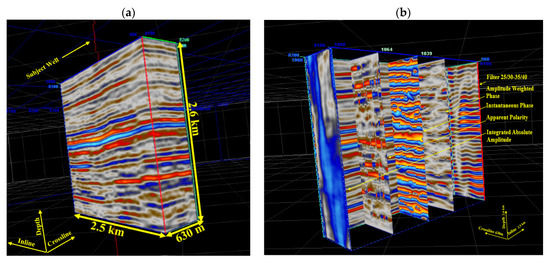
Figure 17. (a) 3D seismic cube used for extracting the employed attributes at the well location; (b) Employed seismic attributes.

Table 10. Properties of the employed data pairs for estimating petrophysical properties from the seismic attributes by both statistical and deep learning models.

Target Curve	Permeability	Porosity
Number of input variables	8	8
Total No. of available data pairs	231	355
No. of training data	185	295
No. of test data	46	60
No. of neurons in the hidden layer	20	20
Iteration the best ANN model was achieved	265	94
Optimal number of trees for statistical Bag ensembles	17	72
Optimal number of trees for statistical LSBoost ensembles	200	200

Table 11. Performance of the employed algorithms in estimating petrophysical properties from the post-stack seismic data.

Target NMR Curve	Permeability		Porosity
Model Performance	MSE	R2	MSE	R2
Bag ensemble	3.95 × 10−2	0.9965	2.59 × 10−1	0.9807
LSBoost ensemble	3.89 × 10−2	0.9950	6.19 × 10−1	0.9525
Artificial neural network	2.13 × 10−2	0.9965	5.20 × 10−1	0.9625

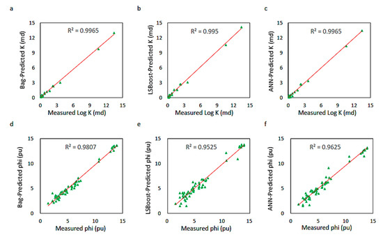
Figure 18. Correlations of the statistically and intelligently estimated permeability (a–c), and porosity (d–f) with the measured values in the unconventional gas field of the Qinshui Basin of China.

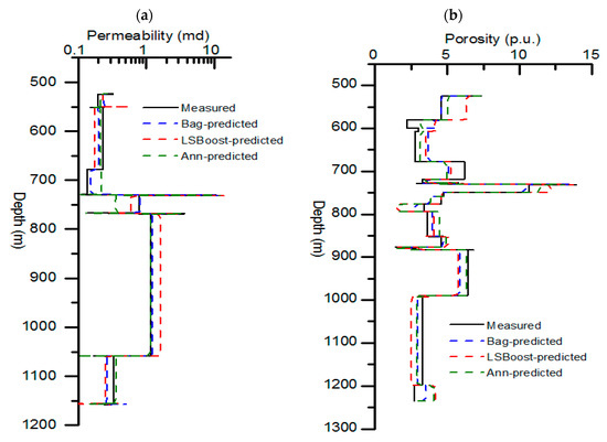
Figure 19. Measured (black), Bag-predicted (blue), LSBoost-predicted (red), and deep learning-predicted (green) curves of permeability (a) and porosity (b) in the unconventional coal reservoir. The stepped representation provides the comparison among the average permeability at different sections of the well, i.e., low permeable and highly permeable sections.

As mentioned earlier, throughout the modeling procedure, porosity was used as the benchmark to guarantee the reliability of the models. Figure 20 represents the 3D porosity cube around one of the subject wells estimated using the statistical Bag ensemble which was evaluated using the original seismic attributes. The agreement of the measured data and the Bag-predicted porosity cube verified the performance of the statistical methods.

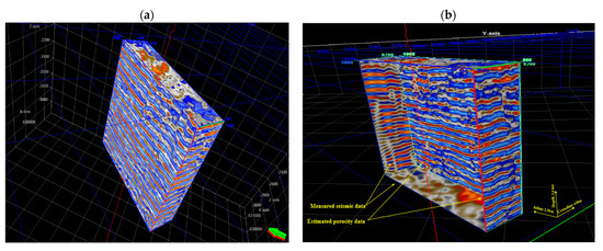
Figure 20. (a) 3D porosity cube around one of the subject wells estimated using the statistical Bag ensemble; (b) Evaluation of the estimated porosity cube (right, front, and surface walls) using a measured 3D seismic attribute, i.e., frequency filter. The satisfying agreement of the statistical model’s result with the measured data proves the reliability of the technique.

4.3. Limitations of the Present Study

The most notable limitation of the present study was applying the research idea merely to coal samples. Nevertheless, other kinds of conventional and unconventional reservoir rocks should also be studied to characterize the detailed contribution of the pore types to the elastic wave velocity. Moreover, a higher number of core samples and a higher number of saturation states would also increase the accuracy of the obtained results. Meanwhile, the present study only investigated two kinds of statistical algorithms and the others are yet to be studied.

5. Conclusions

In the present study, the contribution of different pore types to the elastic P-wave’s velocity was characterized. These results were used to determine the relationship between the bin porosities of the NMR test and the elastic wave velocity under the effect of water saturation. Accordingly, the seismic attributes were successfully used to produce artificial NMT T₂ curves with acceptable accuracy. Moreover, the statistical ensembles were investigated as an alternative tool for the estimation of petrophysical properties and proved as good as the deep learning approach. After all, the research came to the following conclusions:

• Both statistical ensembles and intelligent techniques proved efficient in the case of this research study.
• The performance of the soft-computing techniques strongly depends on the quality and type of input data. Such a conclusion highlights the importance of choosing the best input data when using these techniques.
• When using soft-computing procedures for reservoir characterization, more sensitivity should be shown to unconventional reservoirs according to their more complicated petrophysical properties. However, Geological complexity does not necessarily act as an obstacle to weaken the functionality of these algorithms.
• The seismic wave is composed of three main components which are phase, frequency, and amplitude. Therefore, in any study involving the seismic attributes, it is better to consider the attributes in such a way that one representative of each class is included inside the attribute category. This approach could help to obtain reliable results.
• When making the final decision as to select a model for upscaling purposes, comprehensive consideration of its features and variables including error range, correlation, availability of the inputs, and the requisite amount of the training data and memory is required.

Finally, the authors believe that the ideas introduced in the present study provide new insights for a deeper understanding of the hydrocarbon reservoirs and facilitate comprehending the reciprocal interactions of seismic and magnetic resonance phenomenon within the porous media of the reservoir rock. These ideas are more highlighted in complex pore systems as carbonate reservoirs, which could be suggested as the topic of a future study. Moreover, despite all the advancements, deep learning in the service of petrophysical modeling is still at the be beginning of the way and has got its particular challenges that need to be solved.

References

- Davarpanah, A.; Mirshekari, B.; Behbahani, T.J.; Hemmati, M. Integrated production logging tools approach for convenient experimental individual layer permeability measurements in a multi-layered fractured reservoir. J. Pet. Explor. Prod. Technol. 2018, 8, 743–751. [Google Scholar] [CrossRef]
- Davarpanah, A.; Mirshekari, B.; Razmjoo, A. A parametric study to numerically analyze the formation damage effect. Energy Explor. Exploit. 2019, 38, 555–568. [Google Scholar] [CrossRef]
- Zhu, M.; Yu, L.; Zhang, X.; Davarpanah, A. Application of Implicit pressure-explicit saturation method to predict filtrated mud saturation impact on the hydrocarbon reservoirs formation damage. Mathematics 2020, 8, 1057. [Google Scholar] [CrossRef]
- Yan, W.; Sun, J.; Golsanami, N.; Li, M.; Cui, L.; Dong, H.; Sun, Y. Evaluation of wettabilities and pores in tight oil reservoirs by a new experimental design. Fuel 2019, 252, 272–280. [Google Scholar] [CrossRef]
- Golsanami, N.; Sun, J. Developing a new technique for estimating NMR T1 and T2 relaxations. In Proceedings of the International Geophysical Conference, Qingdao, China, 17–20 April 2017; pp. 1202–1205. [Google Scholar] [CrossRef]
- Sun, T.; Yan, W.; Wang, H.; Golsanami, N.; Zhang, L. Developing a new NMR-based permeability model for fractured carbonate gas reservoirs. J. Nat. Gas Sci. Eng. 2016, 35, 906–919. [Google Scholar] [CrossRef]
- Dong, X.; Shen, L.W.; Golsanami, N.; Liu, X.; Sun, Y.; Wang, F.; Shi, Y.; Sun, J. How N2 injection improves the hydrocarbon recovery of CO2 HnP: An NMR study on the fluid displacement mechanisms. Fuel 2020, 278, 118286. [Google Scholar] [CrossRef]
- Golsanami, N.; Kadkhodaie-Ilkhchi, A.; Sharghi, Y.; Zeinali, M. Estimating NMR T2 distribution data from well log data with the use of a committee machine approach: A case study from the Asmari formation in the Zagros Basin, Iran. J. Pet. Sci. Eng. 2014, 114, 38–51. [Google Scholar] [CrossRef]
- Golsanami, N.; Sun, J.; Zhang, Z. A review on the applications of the nuclear magnetic resonance (NMR) technology for investigating fractures. J. Appl. Geophys. 2016, 133, 30–38. [Google Scholar] [CrossRef]
- Eslami, M.; Kadkhodaie-Ilkhchi, A.; Sharghi, Y.; Golsanami, N. Construction of synthetic capillary pressure curves from the joint use of NMR log data and conventional well logs. J. Pet. Sci. Eng. 2013, 111, 50–58. [Google Scholar] [CrossRef]
- Coates, G.R.; Xiao, L.; Prammer, M.G. NMR Logging Principles and Applications; Halliburton Energy Services Publication: Houston, TX, USA, 1999. [Google Scholar]
- Yasin, Q.; Du, Q.; Ismail, A.; Shaikh, A. A new integrated workflow for improving permeability estimation in a highly heterogeneous reservoir of Sawan Gas Field from well logs data. Géoméch. Geophys. Geo Energy Geo Resour. 2018, 5, 121–142. [Google Scholar] [CrossRef]
- Ismail, A.; Yasin, Q.; Du, Q.; Bhatti, A.A. A comparative study of empirical, statistical and virtual analysis for the estimation of pore network permeability. J. Nat. Gas Sci. Eng. 2017, 45, 825–839. [Google Scholar] [CrossRef]
- Ismail, A.; Yasin, Q.; Du, Q. Application of Hydraulic flow unit for pore size distribution analysis in highly heterogeneous sandstone reservoir: A case study. J. Jpn. Pet. Inst. 2018, 61, 246–255. [Google Scholar] [CrossRef]
- Du, Q.; Yasin, Q.; Ismail, A.; Sohail, G.M. Combining classification and regression for improving shear wave velocity estimation from well logs data. J. Pet. Sci. Eng. 2019, 182, 106260. [Google Scholar] [CrossRef]
- Hu, X.; Xie, J.; Cai, W.; Wang, R.; Davarpanah, A. Thermodynamic effects of cycling carbon dioxide injectivity in shale reservoirs. J. Pet. Sci. Eng. 2020, 195, 107717. [Google Scholar] [CrossRef]
- Davarpanah, A.; Nassabeh, S.M.M.; Mirshekari, B. Optimization of Drilling parameters by analysis of formation strength properties with utilization of mechanical specific energy. Open J. Geol. 2017, 7, 1590–1602. [Google Scholar] [CrossRef]
- Hamada, G.M.; Elshafei, M. Neural network prediction of porosity and permeability of heterogeneous gas sand reservoirs. Nafta 2010, 61, 451–460. [Google Scholar]
- Mohaghegh, S.; Richardson, M.; Ameri, S. Use of intelligent systems in reservoir characterization via synthetic magnetic resonance logs. J. Pet. Sci. Eng. 2001, 29, 189–204. [Google Scholar] [CrossRef]
- Labani, M.M.; Kadkhodaie-Ilkhchi, A.; Salahshoor, K. Estimation of NMR log parameters from conventional well log data using a committee machine with intelligent systems: A case study from the Iranian part of the South Pars gas field, Persian Gulf Basin. J. Pet. Sci. Eng. 2010, 72, 175–185. [Google Scholar] [CrossRef]
- Hatampour, A.; Schaffie, M.; Jafari, S. Estimation of NMR total and free fluid porosity from seismic attributes using intelligent systems: A case study from an Iranian carbonate gas reservoir. Arab. J. Sci. Eng. 2016, 42, 315–326. [Google Scholar] [CrossRef]
- Iturrarán-Viveros, U.; Parra, J.O. Artificial neural networks applied to estimate permeability, porosity and intrinsic attenuation using seismic attributes and well-log data. J. Appl. Geophys. 2014, 107, 45–54. [Google Scholar] [CrossRef]
- Fattahi, H.; Karimpouli, S. Prediction of porosity and water saturation using pre-stack seismic attributes: A comparison of Bayesian inversion and computational intelligence methods. Comput. Geosci. 2016, 20, 1075–1094. [Google Scholar] [CrossRef]
- Yang, Z.; Pan, X.H.; Yuan, S.Q.; Ji, Z.F. Application of NMR in coal reservoir characterization. Adv. Mater. Res. 2013, 765–767, 2168–2171. [Google Scholar] [CrossRef]
- Rabbani, E.; Davarpanah, A.; Memariani, M. An experimental study of acidizing operation performances on the wellbore productivity index enhancement. J. Pet. Explor. Prod. Technol. 2018, 8, 1243–1253. [Google Scholar] [CrossRef]
- Jiang, L.; Zhao, Y.; Golsanami, N.; Chen, L.; Yan, W. A novel type of neural networks for feature engineering of geological data: Case studies of coal and gas hydrate-bearing sediments. Geosci. Front. 2020, 11, 1511–1531. [Google Scholar] [CrossRef]
- Zargar, G.; Tanha, A.A.; Parizad, A.; Amouri, M.; Bagheri, H. Reservoir rock properties estimation based on conventional and NMR log data using ANN-Cuckoo: A case study in one of super fields in Iran southwest. Petroleum 2020, 6, 304–310. [Google Scholar] [CrossRef]
- Yu, B.; Zhao, H.; Tian, J.; Liu, C.; Song, Z.; Liu, Y.; Li, M. Modeling study of sandstone permeability under true triaxial stress based on backpropagation neural network, genetic programming, and multiple regression analysis. J. Nat. Gas Sci. Eng. 2021, 86, 103742. [Google Scholar] [CrossRef]
- Sudakov, O.; Burnaev, E.; Koroteev, D. Driving digital rock towards machine learning: Predicting permeability with gradient boosting and deep neural networks. Comput. Geosci. 2019, 127, 91–98. [Google Scholar] [CrossRef]
- Islam, S.M.A. Investigation of fluid properties and their effect on seismic response: A case study of Fenchuganj gas field, Surma Basin, Bangladesh. Int. J. Oil Gas Coal Eng. 2014, 2, 36–54. [Google Scholar] [CrossRef]
- Rubino, J.G.; Velis, D.R.; Holliger, K. Permeability effects on the seismic response of gas reservoirs. Geophys. J. Int. 2012, 189, 448–468. [Google Scholar] [CrossRef]
- Goloshubin, G.; Silin, D.; Vingalov, V.; Takkand, G.; Latfullin, M. Reservoir permeability from seismic attribute analysis. Lead. Edge 2008, 27, 376–381. [Google Scholar] [CrossRef]
- Wang, G.; Li, J.; Liu, Z.; Qin, X.; Yan, S. Relationship between wave speed variation and microstructure of coal under wet conditions. Int. J. Rock Mech. Min. Sci. 2020, 126, 104203. [Google Scholar] [CrossRef]
- Yu, G.; Vozoff, K.; Durney, D.W. The influence of confining pressure and water saturation on dynamic elastic properties of some Permian coals. Geophysics 1993, 58, 30–38. [Google Scholar] [CrossRef]
- Garia, S.; Pal, A.K.; Ravi, K.; Nair, A.M. A comprehensive analysis on the relationships between elastic wave velocities and petrophysical properties of sedimentary rocks based on laboratory measurements. J. Pet. Explor. Prod. Technol. 2019, 9, 1869–1881. [Google Scholar] [CrossRef]
- Yun, W.A.N.G.; Xiao-Kai, X.U.; Yu-Gui, Z.H.A.N.G. Ultrasonic elastic characteristics of six kinds of metamorphic coals in China under room temperature and pressure conditions. Chin. J. Geophys. 2016, 59, 350–363. [Google Scholar] [CrossRef]
- Marcía-González, M.; Towle, G. Measurement of elastic wave velocities in coal. Boletín Geol. 2006, 28, 81–95. [Google Scholar]
- Greenhalgh, S.; Emerson, D. Elastic properties of coal measure rocks new south wales. Explor. Geophys. 1986, 17, 157–163. [Google Scholar] [CrossRef]
- Morcote, A.; Mavko, G.; Prasad, M. Dynamic elastic properties of coal. Geophysics 2010, 75, E227–E234. [Google Scholar] [CrossRef]
- Ogilvie, S.R.; Cuddy, S.; Lindsay, C.; Hurst, A. Novel methods of permeability prediction from NMR tool data. Dialog Lond. Petrophys. Soc. 2002, 141, 1–14. [Google Scholar]
- Ge, X.; Wang, H.; Fan, Y.; Cao, Y.; Chen, H.; Huang, R. Joint inversion ofT1–T2spectrum combining the iterative truncated singular value decomposition and the parallel particle swarm optimization algorithms. Comput. Phys. Commun. 2016, 198, 59–70. [Google Scholar] [CrossRef]
- Ge, X.; Chen, H.; Fan, Y.; Liu, J.; Cai, J.; Liu, J. An improved pulse sequence and inversion algorithm of T2 spectrum. Comput. Phys. Commun. 2017, 212, 82–89. [Google Scholar] [CrossRef]
- He, W.; Chen, Z.; Shi, H.; Liu, C.; Li, S. Prediction of acoustic wave velocities by incorporating effects of water saturation and effective pressure. Eng. Geol. 2020, 280, 105890. [Google Scholar] [CrossRef]
- Bakhshi, E.; Golsanami, N.; Chen, L. Numerical modeling and lattice method for characterizing hydraulic fracture propagation: A review of the numerical, experimental, and field studies. Arch. Comput. Methods Eng. 2020, 1–32. [Google Scholar] [CrossRef]
- Golsanami, N.; Bakhshi, E.; Yan, W.; Dong, H.; Barzgar, E.; Zhang, G.; Mahbaz, S. Relationships between the geomechanical parameters and Archie’s coefficients of fractured carbonate reservoirs: A new insight. Energy Sources Part A Recover. Util. Environ. Effects 2020. [Google Scholar] [CrossRef]
- Wyllie, M.R.J.; Gregory, A.R.; Gardner, L.W. Elastic wave velocities in heterogeneous and porous media. Geophysics 1956, 21, 41–70. [Google Scholar] [CrossRef]
- Kamel, M.H.; Mabrouk, W.M.; Bayoumi, A.I. Porosity estimation using a combination of Wyllie–Clemenceau equations in clean sand formation from acoustic logs. J. Pet. Sci. Eng. 2002, 33, 241–251. [Google Scholar] [CrossRef]
- Qiang, Z.; Yasin, Q.; Golsanami, N.; Du, Q. Prediction of reservoir quality from log-core and seismic inversion analysis with an artificial neural network: A case study from the Sawan Gas Field, Pakistan. Energies 2020, 13, 486. [Google Scholar] [CrossRef]
- Sun, Z.; Jiang, L.; Jiang, J.; Wu, X.; Golsanami, N.; Huang, W.; Zhang, P.; Niu, Z.; He, X. Parametric study on the ground control effects of rock bolt parameters under dynamic and static coupling loads. Adv. Civ. Eng. 2020, 2020, 1–12. [Google Scholar] [CrossRef]
- Schlumberger. Petrel Software Manual. 2011. Available online: https://www.software.slb.com/products/product-library-v2?product=Petrel&tab=Product%20Sheets (accessed on 18 January 2021).
- MathWorks. Statistics ToolboxTM User’s Guide; The MathWorks, Inc.: Natick, MA, USA, 2011. [Google Scholar]
- The Elements of Statistical Learning. Springer Ser. Stat. 2009, 605–624. [CrossRef]
- Sugiyama, M. Ensemble Learning. Introd. Stat. Mach. Learn. 2016, 343–354. [Google Scholar] [CrossRef]
- Chollet, F. Deep Learning with Python; Manning Publications: New York, NY, USA, 2017; Available online: www.amazon.com/Deep-Learning-Python-Francois-Chollet/dp/1617294438 (accessed on 18 January 2021).
- Hinton, G.E.; Osindero, S.; Teh, Y.-W. A fast learning algorithm for deep belief nets. Neural Comput. 2006, 18, 1527–1554. [Google Scholar] [CrossRef]
- Sohn, I. Deep belief network based intrusion detection techniques: A survey. Expert Syst. Appl. 2021, 167, 114170. [Google Scholar] [CrossRef]
- Savitha, R.; Ambikapathi, A.; Rajaraman, K. Online RBM: Growing Restricted Boltzmann Machine on the fly for unsupervised representation. Appl. Soft Comput. 2020, 92, 106278. [Google Scholar] [CrossRef]
- Yevick, D.; Melko, R. The accuracy of restricted Boltzmann machine models of Ising systems. Comput. Phys. Commun. 2021, 258, 107518. [Google Scholar] [CrossRef]
- Hatistie, T.; Tibshrani, R.; Fridman, J. The Elements of Statistical Learning; Springer International Publishing: Geneva, Switzerland, 2009. [Google Scholar]
- Gao, X.; Zheng, H.; Zhang, Y.; Golsanami, N. tax policy, environmental concern and level of emission reduction. Sustainability 2019, 11, 1047. [Google Scholar] [CrossRef]
- Dong, H.; Sun, J.; Zhu, J.; Liu, L.; Lin, Z.; Golsanami, N.; Cui, L.; Yan, W. Developing a new hydrate saturation calculation model for hydrate-bearing sediments. Fuel 2019, 248, 27–37. [Google Scholar] [CrossRef]
- Dong, H.; Sun, J.; Arif, M.; Golsanami, N.; Yan, W.; Zhang, Y. A novel hybrid method for gas hydrate filling modes identification via digital rock. Mar. Pet. Geol. 2020, 115, 104255. [Google Scholar] [CrossRef]
- Huaimin, D.; Jianmeng, S.; Likai, C.; Naser, G.; Weichao, Y. Characteristics of the pore structure of natural gas hydrate reservoir in the Qilian Mountain Permafrost, Northwest China. J. Appl. Geophys. 2019, 164, 153–159. [Google Scholar] [CrossRef]
Publisher’s Note: MDPI stays neutral with regard to jurisdictional claims in published maps and institutional affiliations. |
© 2021 by the authors. Licensee MDPI, Basel, Switzerland. This article is an open access article distributed under the terms and conditions of the Creative Commons Attribution (CC BY) license (http://creativecommons.org/licenses/by/4.0/).