Impact of Heat Transfer on Transient Stress Fields in Power Plant Boiler Components

Abstract

In boilers operating in modern power plants, thick-walled elements of complex shapes, such as valves, superheater headers, T-pipes, Y-pipes, four-way pipes, and elbows, are especially prone to fatigue processes. Higher operation parameters and more frequent startups may speed up fatigue damage in these elements. Such damage is a local phenomenon and is caused by thermomechanical fatigue (TMF). This paper presents a method designed for predicting the behavior of components subjected to variable temperature and mechanical loading conditions. This method combines the results of measurements of operating parameters of devices under industrial conditions with those obtained using finite element modeling (FEM). Particular attention was given to the influence of the time-dependent heat transfer coefficient on the local thermomechanical stress–strain behavior of the material. It was stated that heat transfer conditions have a significant impact on local transient stresses and depend on the operation parameters of boilers. Consistency of the temperature changes as a function of time, determined in industrial conditions and calculated on the basis of the model approach, was obtained. This developed and described in the work approach enables defining the conditions of heat transfer on the surface of models of considered components.

1. Introduction

The changes currently being seen in the power sector industry—and manifested in a marked increase in the use of renewable energy sources—are increasingly common worldwide, with the conditions and consequences of these changes becoming areas of research and analysis on both domestic and global scales. Points of interest range from technological and economic issues of implementing new methods of obtaining energy to problems related to increasing the efficiency of the existing conventional energy installations. While many countries continue to rely predominantly on fossil fuels, such as coal, oil and natural gas for power generation, it should be noted that more attention is paid to the efficiency of the newly introduced energy generation devices [1,2,3]. This efficiency is considered in economic terms and in connection with the impact of energy generation and consumption on CO₂ emissions and climate change.

On a global scale, the direction of further developments in the power sector seems to be clearly defined. What remains to be determined is how to implement these changes, their time frames and the economic requirements for the implementation of new technologies and investments in available ecological methods of generating energy. Assuming no major political obstacles to progress, it can be assumed that most countries in the world will need a long-term transition period in which conventional power plants will work alongside systems based on renewable energy sources. The compatibility of various systems would raise a number of new technical problems.

In countries whose primary energy systems are still predominantly based on coal, there are many power plants that have been in operation for years, and their equipment has often reached a significant degree of wear. For safety reasons, it is necessary to assess their technical condition in order to determine the possibility of further operation, which would result in either the need for modernization or the exclusion from further operation in the network. Due to the limited economic possibilities, in many cases, these power plants will need to operate for a certain period of time during the transitional period. Their use in a system, a significant part of which are renewable energy sources, including wind and solar power plants, entails the necessity of adjusting the amount of generated energy on an ongoing basis to changes in the demand for the power they generate. Such changes cause frequent shutdowns and restarts of devices in these power plants or oscillations of the power obtained from them.

The conventional power generation industry is affected by new trends in energy demand. In the near future, the equipment in fossil-fuel power plants is going to be adjusted to new operating conditions, from continuous operation at constant loads to adaptation to changes in power demand, with dynamic impact phenomena playing a crucial role. Consequently, the assessment of the current endurance and durability of energy installations requires taking into account, to a greater extent than it was the case at the design stage, the issues of load variability, including the issues of the impact of loading on the fatigue life of the materials.

With modern high-efficiency power stations, i.e., supercritical and ultra-supercritical power plants, a new approach to the issue of their endurance assessment and durability forecasting is also required due to changes in the operating conditions of energy systems and the increased operating parameters of high-efficiency power-generation equipment. High temperatures and pressures in boiler components necessitate the use of new high creep-resistant materials under steady and variable loads. Such creep properties can be ensured by new materials with chemical compositions different from those in the previously used materials, and most often with different physical properties as well.

New heat-resistant alloys, as compared to the materials traditionally used in power-generation devices, tend to show higher values of the thermal expansion coefficient and lower thermal conductivity. Both properties favor the formation of thermal stresses caused by an uneven temperature field under steady and transient heat flow conditions.

The previous and current methods of strength assessment of power-generation components take into account the calculations of durability and the degree of damage based on estimated values of the degree of nonuniformity of temperature fields and approximate formulas enabling the estimation of the magnitude of thermal stresses. On their basis, it is possible to assess the expected effects of changes in working conditions and evaluate the application of new materials in components of energy devices. However, such an assessment is largely subject to uncertainty related to the adopted simplifications.

The need to ensure safe operating conditions of devices in the energy industry currently subject to rapid changes requires the development or modification of strength assessment methods for components subjected to the impact of variable temperatures in order to more precisely capture the impact of stresses caused by uneven temperature fields on fatigue phenomena and to estimate the probability of defects under mechanical and thermal loads.

One crucial aspect of this complex problem is the assessment of the impact of heat transfer conditions on the surface of pressure vessels on the time-dependent stress–strain behavior. In the methodology for calculation of temperatures and thermal stresses used in the currently binding standards, constant values of the heat transfer coefficient, different for steam and water, are assumed in this case [4]. Under operating conditions, the temperature, the flow rate and steam pressure are measured simultaneously, and temperature measurements are taken at selected points of the component parts. Therefore, it is possible to assess the extent to which such an assumption affects the accuracy of assessments of local temperature values and the estimation of the unevenness of its distribution. In such a case, computer calculation methods can be used, including the finite element method (FEM), in order to determine the time-varying temperature distribution under the assumed boundary conditions. The calculations made in this way show significant discrepancies between the temperatures measured at selected points of the elements and the calculated values.

In the technical literature on the fatigue of the materials of power equipment components, one can find studies on the analysis of temperature fields and thermal stresses caused by changes in the operating parameters of these devices [5,6,7,8,9,10,11,12,13]. There are considered examples of elements for which data on time-varying mechanical and thermal loads were available. In the test results documented in the form of publications, constant values of the heat transfer coefficient are adopted [5,6], or attempts are made to determine the thermal load as a function of time. The heat transfer coefficient on the surface of the considered elements was determined on the basis of variable parameters of the medium flowing through them, including temperature and flow rate, using computer programs, including computational fluid dynamics (CFD) methods [7,8,9,10]. Earlier works by the authors also used methods of matching the heat transfer coefficient to the results of local temperature measurements in order to obtain consistency of the calculated temperature distributions and the measurement results [11,12]. However, there are no extensive studies devoted to the verification of the obtained calculation results on the basis of the results of tests in industrial conditions. Relatively few works were devoted to the problem of determining the heat transfer coefficient for devices of complex shape under the conditions of time-varying elevated temperature, pressure and flow rate of steam in elements of energy boilers.

Most often, considerations of this type relate to flow in pipes and include, among others, studies [13,14,15]. The paper [13] compares correlations implemented for heat-transfer in case of super critical water (SCW). It has been shown that the results of these correlations may differ more than twice it led to the conclusion that an accurate SCW heat-transfer correlation is vital for a wide range of operation parameters of power plant. The paper [13] summarizes the results of research performed for various flow geometries, and different fluids, but mainly for water. The paper [14] contains an analysis of heat-transfer for supercritical water flow in bare vertical tubes. Experimental data have been taken from research performed in Russia. Based on these results a new heat-transfer correlation was worked out. Conditions of the research, from which the experimental data have been taken, were similar to those in a supercritical water-cooled nuclear reactor (SCWR). The k–ω turbulence model was presented in the paper [15], and computations of heat transfer in vertical tubes were carried out using the ANSYS-CFX code. Sensitivity study of the computation results to operational conditions and the Prandtl number was done. It was stated that the Prandtl number had a significant influence on the tube’s wall temperature.

The phenomenon of heat transfer in components of a complex shape was analyzed in the paper [16]. Methods for monitoring the thermal stresses in chosen components of power plants under operation conditions were described. Two different methods have been used. First of them has been based on the measurements of the unsteady temperature distribution in the components. This distribution was determined by measuring the wall temperature at several points located on the outer surface of the elements. The inverse problem of heat conduction has been solved and the time dependent temperature distribution in the component was determined. An advantage of this approach is that there was no need to know the temperature of the fluid and the heat transfer coefficient, when the first method was used. Stresses in a component with a complicated shape were computed using the finite element method (FEM) in the second method. Fluid temperature was experimentally estimated and heat transfer coefficient was assumed as known. The paper [16] also describes an original numerical-experimental method of determination of the heat transfer coefficient based on the solution of the 3D-inverse heat transfer problem. The wall temperature was measured at six points located close to the inner surface or local temperature distribution was measured on the outer surface of the component. The heat transfer coefficient on the inner surface was determined based on these experimental results. Examples of application of these methods for stresses computations in the superheater header and the header of the steam cooler in a power plant were discussed.

Summarizing the presented state of knowledge, it can be noted that the problem issue of the correct definition of heat transfer conditions in the problems of determining thermal stresses in elements of energy devices has not been fully solved so far. Despite the existing attempts to use in this case CFD methods, there are still significant discrepancies between the results of methods proposed in the technical literature and the results of measurements in laboratory and industrial conditions. There is a limited number of works presenting the results of research on heat transfer phenomena in industrial conditions in the transient operating state of thick-walled elements of power devices, in which thermal stresses are an important factor determining their durability.

It seems still justified to ask the question to what extent the assumption of a constant value of heat transfer coefficient affects the obtained results. If the discrepancies are significant, an attempt should be made to determine the heat transfer coefficient more precisely in order to obtain better compatibility of computational and experimental data. As there are many different proposals in the technical literature regarding the method of defining the heat transfer conditions on the surfaces of the considered elements, and the discrepancies between the results of these methods are significant [13], tests in industrial conditions still seem to be the basic criterion for assessing the correctness of a given method. The paper presents a method of defining the time-varying heat transfer coefficient in a power boiler element, ensuring the most accurate representation of the variable temperature field in its volume. This method is based on the combination of the approach based on the calculation of the Nusselt number along with matching the value of the heat transfer coefficient in selected time intervals to the results of temperature measurements in the volume of the element.

Here were compared the results of temperature calculations made by the finite element method for the heat transfer coefficient adopted in accordance with the standards and determined using the proposed method.

In this case, the study uses exemplary components of power boilers for which data were available in relation to their geometric features and material properties, as well as the results of measurements of operating parameters under operating conditions. This paper focuses on methodological aspects, striving for the best representation of the time-varying temperature distribution in these components. Although the work at the present stage focuses mainly on the problem of determining the time-varying temperature field, its purpose is then to apply the obtained results to determine transient thermal stress fields in the examined elements of energy devices, necessary to assess their current strength and durability.

2. Characteristics of the Components

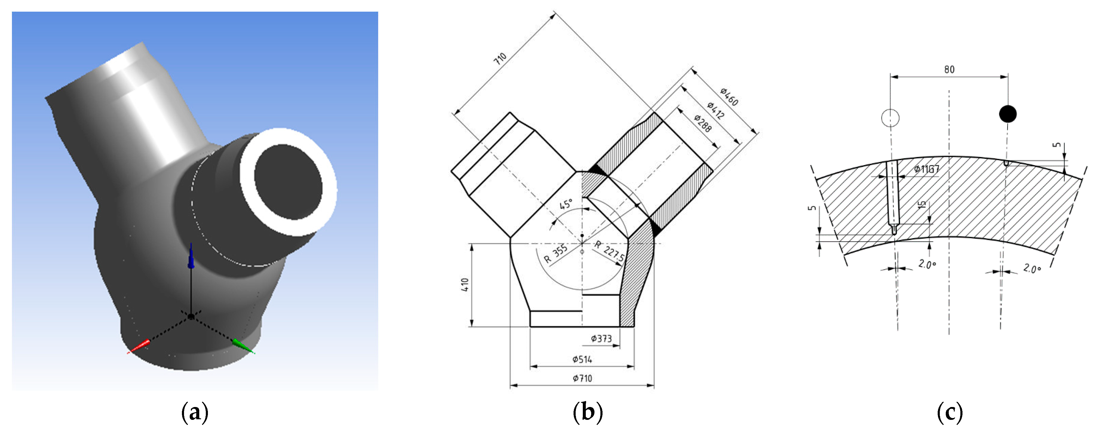
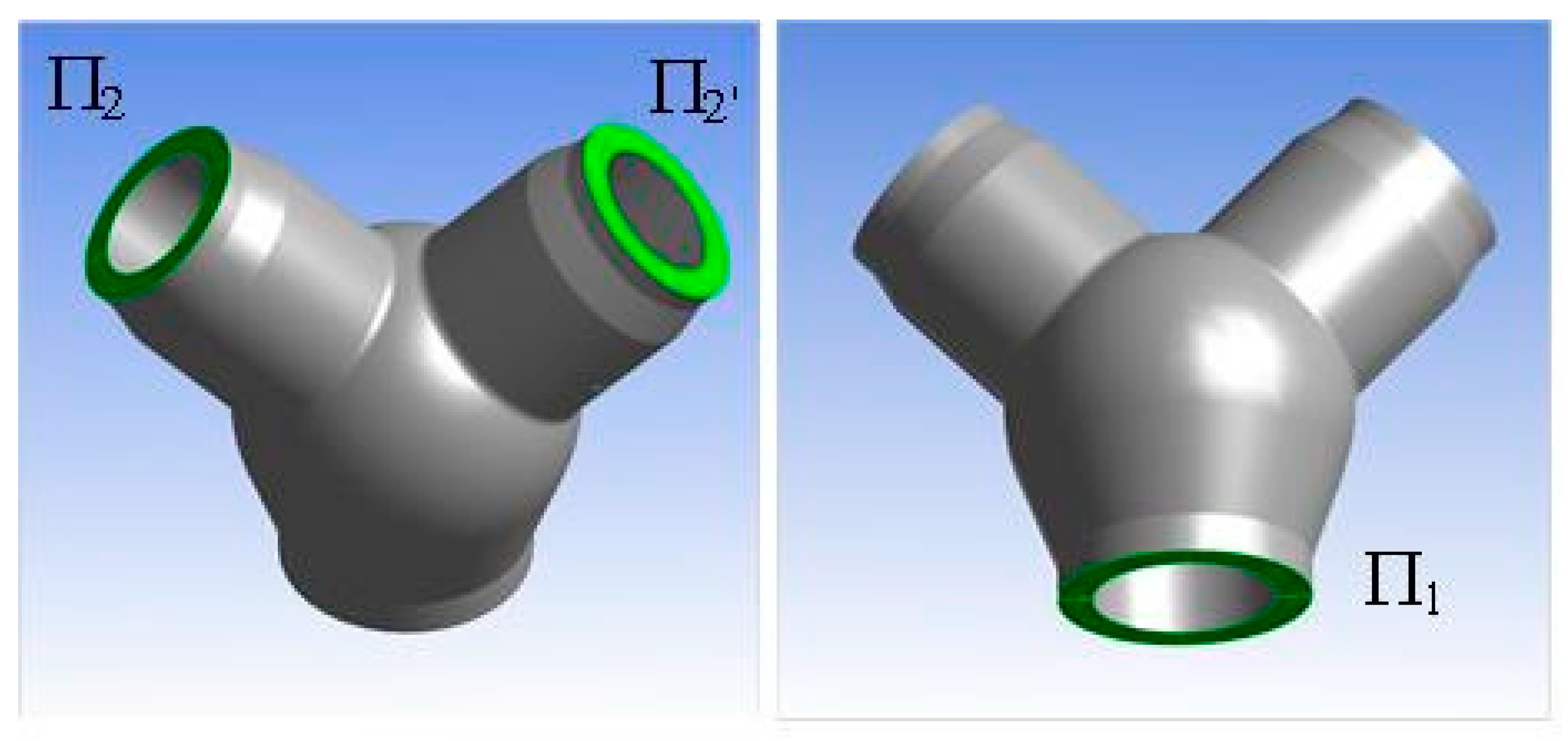
For the analysis of the heat-flow phenomena and the associated time-varying temperatures and stress distributions, a thick-walled component in a power pipeline operating in a unit of 360 MW was used. It was a live steam pipeline at an operating temperature of 540 °C and a nominal pressure of 18.4 MPa. This pipeline is made of 14MoV6-3 steel and connects the boiler with the turbine in the power unit. In its upper part, there is a Y-shaped junction connecting the two parts of the pipeline leading from the boiler into a section running vertically downwards and then branching at the level below the turbines to sections supplying steam to the turbine valves. Figure 1a shows an isometric view of the Y-shaped junction. 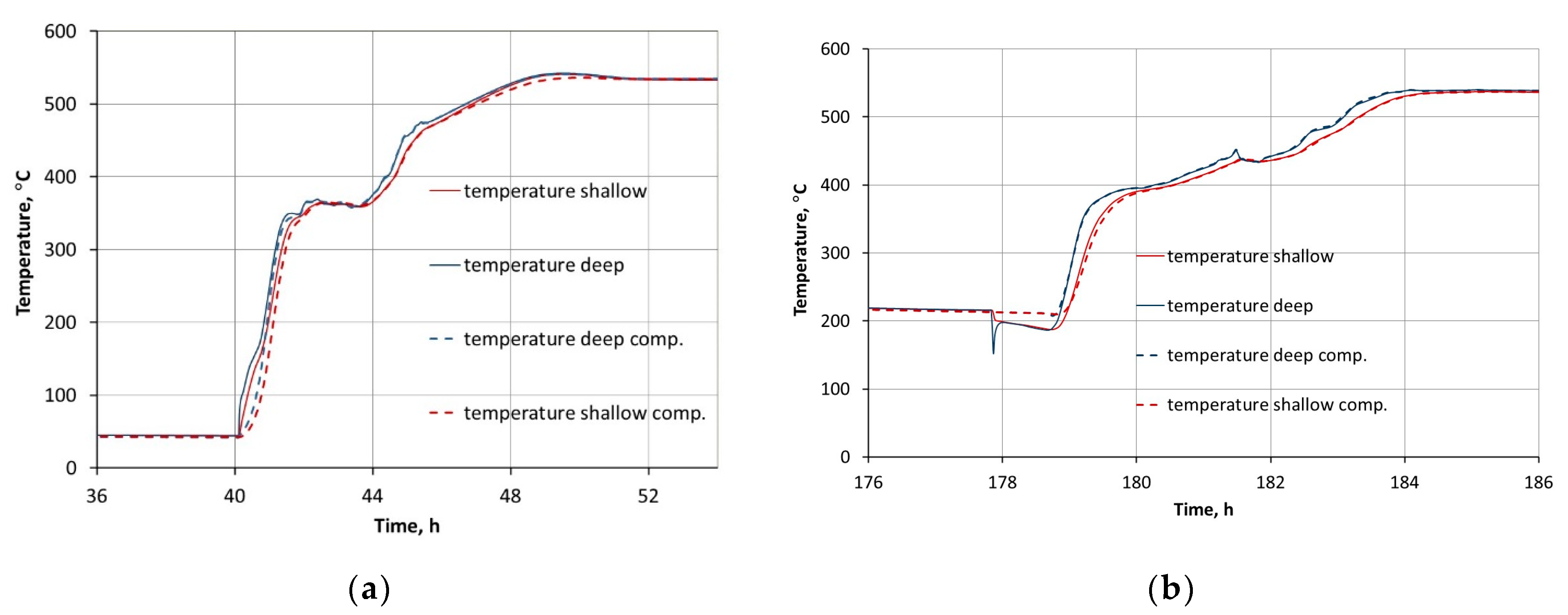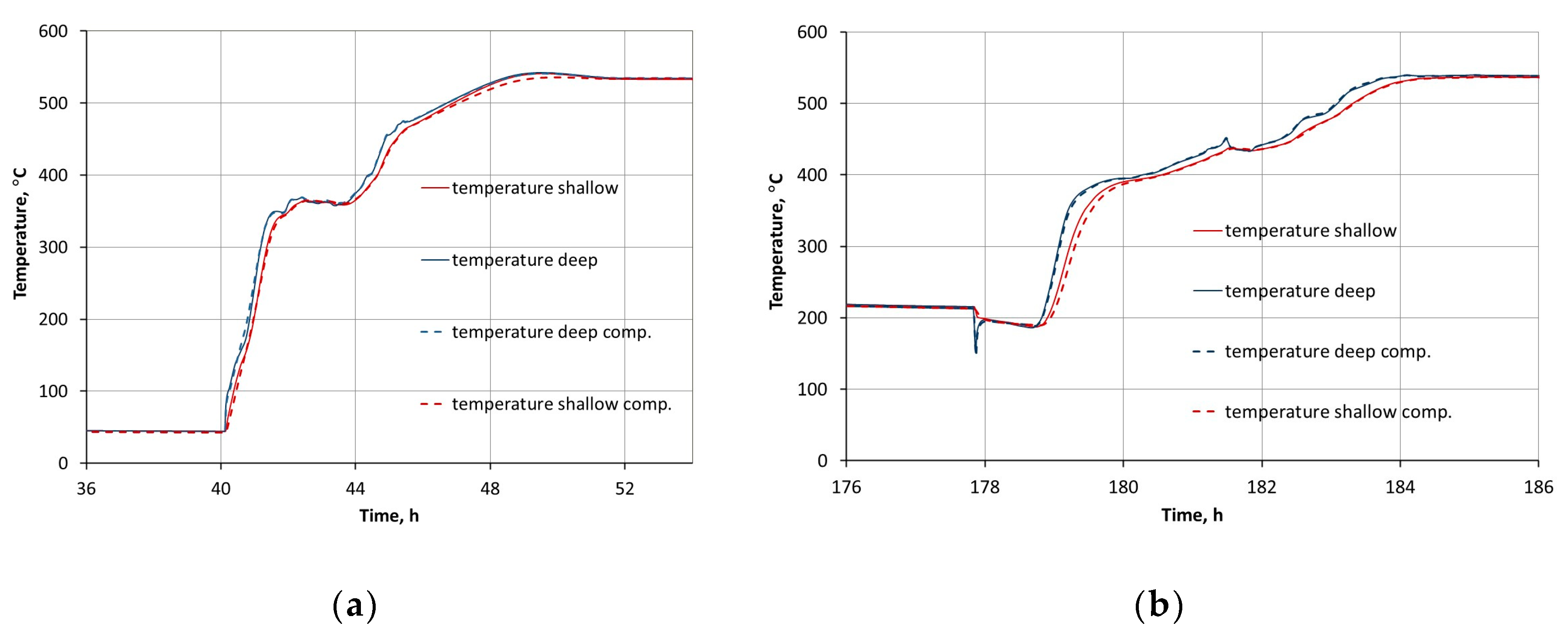Figure 1b shows a cross-section of this Y-junction and its major dimensions. The thermocouples used for temperature measurements are located in selected points of the junction (Figure 1c), in the spherical part of the junction, in which two holes are drilled in the same horizontal plane. The shallow one ends 5 mm below the outer surface and the other 5 mm above the inner surface (deep in relation to the outer surface). The thermocouples measure the temperatures at the bottom parts of the holes.

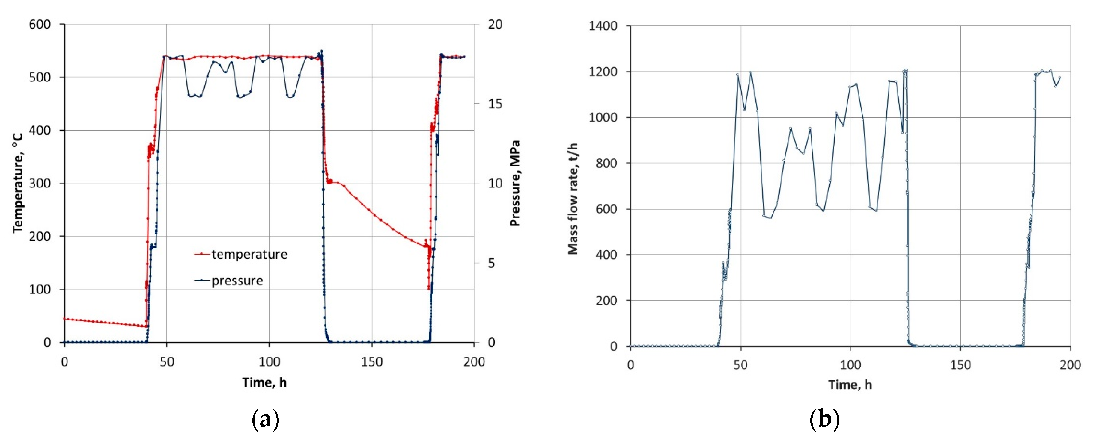
When starting the analysis, the results available included: steam temperature measurements downstream of the boiler from which the pipeline comes out, the temperature of the Y-shaped junction at points located shallow and deep, steam pressure measurements, and steam mass flow rates. These data were obtained over a period of many years of the operation of the pipeline. For this analysis, one representative period of the operation of the installation was selected, including the startup, a selected steady operation period, the shutdown, and a hot startup. In the case under consideration, the restarting took place after the pipeline had cooled down to a temperature of about 200 °C. The time histories of pressures, steam temperatures and mass flow rates in the considered period of operation are shown in Figure 2.

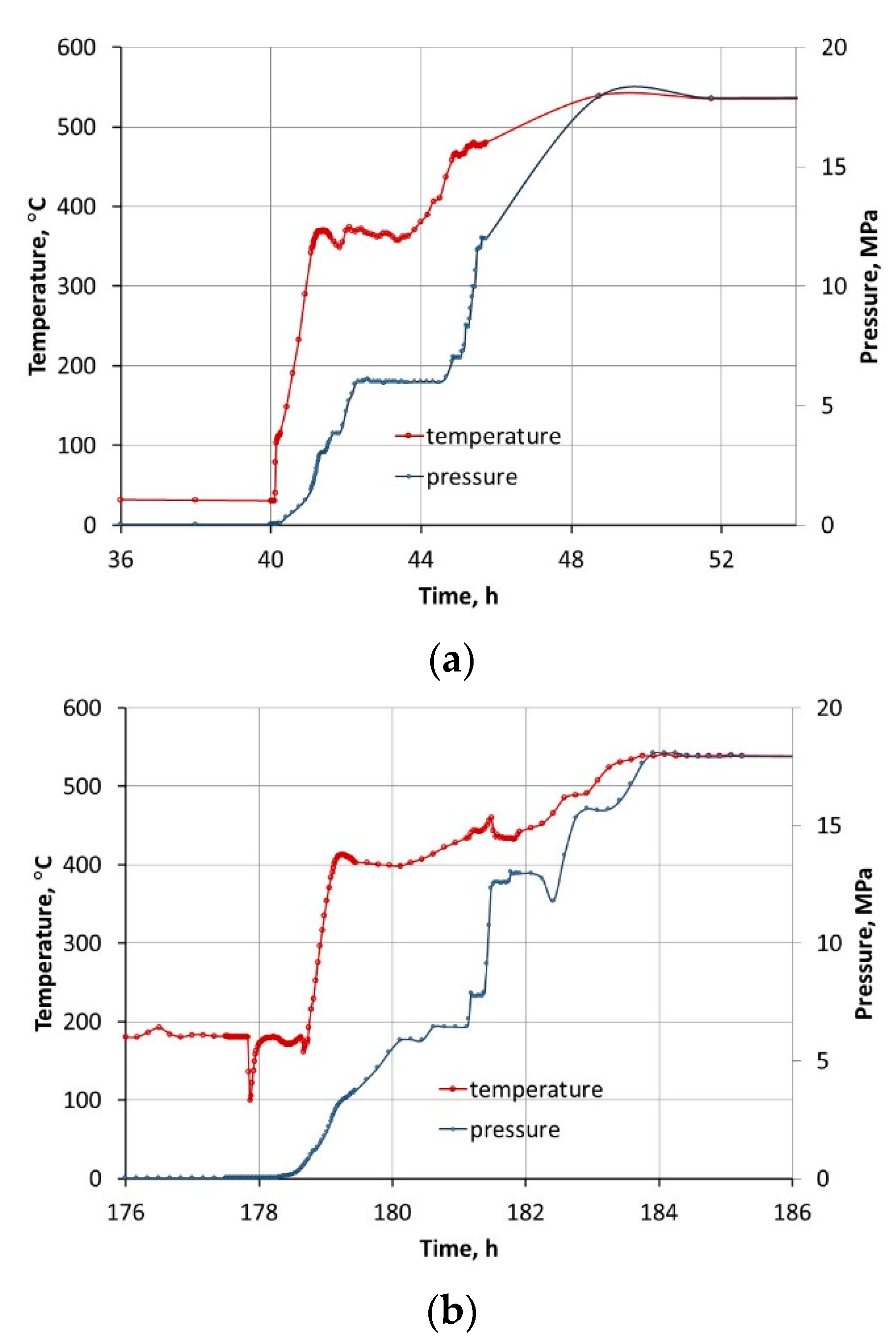
Figure 3 shows selected fragments of the graphs in Figure 2a in order to present detailed operation of the pipeline in transition periods. These periods are marked by considerable changes in temperature. These changes—as recorded for the considered component—cause large thermal gradients and accompanying thermal stresses, the determination of which is the subject of this study.

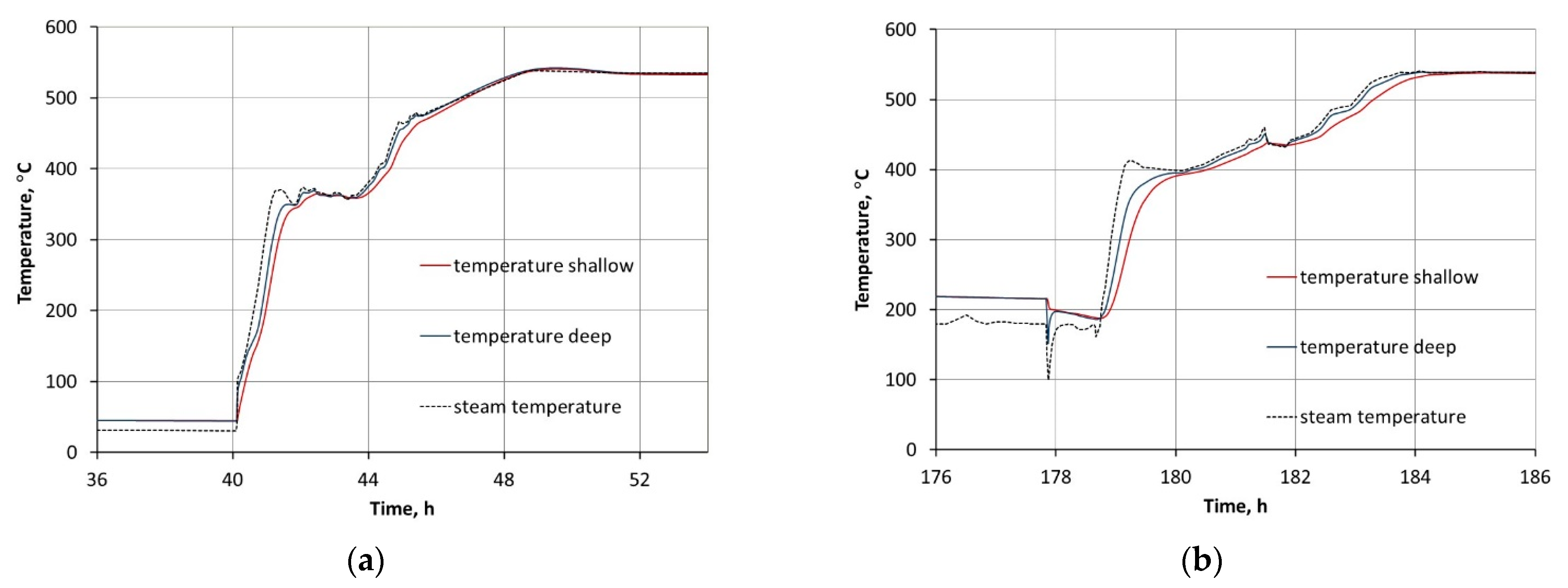
The temperature measurement system, which includes thermocouples located in the Y-shaped junction, is used for the current control of the installation operation, including the assessment of the time-varying differences between the temperatures of the inner and outer surfaces in order to estimate the stress values caused by the uneven temperature fields. Under industrial conditions, such stresses are assessed on the basis of the dependencies included in the standard [4], which assume a simplified shape of the component and elastic model of the material. The influence of the temperature field on the local properties of the material of the component under consideration is not taken into account. Temperature changes in selected periods measured by thermocouples located shallow and deep under the outer surface of the Y-shaped junction are shown in Figure 4, which also presents the characteristics of steam temperature changes as a function of time.

The characteristics of temperature changes as a function of time at the shallow and deep located points of measurement in the Y-shaped junction below its external surface will be used in the further part of the paper to assess the compatibility of the calculation results made with the use of models with the results of tests conducted under industrial conditions.

3. Models for Calculation of Temperature and Stress Fields

The aim of the analysis was to develop a method for the determination of time-varying temperature distribution and the accompanying stress distribution in the volume of the considered junction while taking into account the influence of temperatures on the properties of the material. These distributions significantly depend on heat transfer conditions on the surfaces of the component under consideration. The method for the assessment of these conditions and the way of defining them is considered in work with the use of computer modeling methods, including FEM. When analyzing the behavior of the junction in question, the Ansys program was used for the calculations of temperatures and stress fields.

On the basis of the technical documentation of the geometric features of the Y-shaped junction, a model was developed. The junction was separated from the pipeline by means of three sections, as shown in Figure 5, with planes Π₁, Π₂ and Π_2’. The interactions of transverse forces, axial forces, bending and torsional moments on the cross-sectional planes from the remaining part of the pipeline were disregarded. These interactions result from the impact of the time-varying distribution of temperature along the pipeline, pre-strains and assembly stresses on the magnitude of internal forces that occur in the installation as a result of restricting its global displacements by means of pipeline hangers and supports. However, axial stresses caused by the pressure inside the pipeline were taken into account. Considering the temperature fields, it was assumed that the cross-sections of infinitely long sections of pipes connected to this junction have the same temperature fields as those at the respective sections ₁, ₂ i _2′. Therefore, a zero value of the heat flux was assumed perpendicular to the planes of intersections.

The physical properties of the material of the junction adopted for this analysis were based on the data available in the literature [17,18], which were further prepared as input data for the finite element method program.

Table 1. Properties of steel grade 14MoV6-3.

Temperature T, °C	20	100	200	300	400	500	600
Young’s modulus, E 10−5, MPa	2.12	2.07	1.99	1.92	1.84	1.75	1.64
Yield stress, Rp0,2, MPa	330	305	267	225	209	200	160
Thermal conductivity,λ,W/(mK)	46.3	47.1	46.2	44.1	41.3	38.6	35.9
Thermal expansion coefficient,β106, 1/K	11.5	12.1	12.7	13.2	13.6	14	14.4
Specific heat, cp, kJ/kgK	0.461	0.496	0.533	0.568	0.611	0.677	0.778

lists the physical and mechanical properties of the junction material, 14MoV6-3 steel, used in the calculations. These properties are presented as a function of temperature in centigrade.

Figure 6a shows the temperature dependence of Young’s modulus and the yield point R_p0.2, and Figure 6b shows the stress–plastic strain curves in different temperatures. These curves were used to develop a material model for stress and strain calculations. These calculations applied the multilinear kinematic hardening model based on the Besseling model [19,20,21], which assumes that the elementary volume of an elastic–plastic material is composed of different parts: smaller sub-volumes with the same elastic modulus and total strain, but different values of the yield point. It was assumed that each elemental volume displays an ideal elastic–plastic behavior. By combining these elements, a model was created for the representation of complex behaviors, such as the stress–strain curve (showing the relationship between the change in stress with the increase in strain) composed of many sections, which exhibits kinematic hardening with the Bauschinger effect. Elementary volume-weight fractions were determined by fitting the material response to the curve determined under uniaxial strain conditions. Steel 14MoV6-3 was introduced into the model as an elastic–plastic material with kinematic hardening and temperature-dependent properties such as Young’s modulus and the linear thermal expansion coefficient. The temperature-dependent hardening curves of steel 14MoV6-3, shown in Figure 6b, were developed on the basis of the tensile curves.

The calculations also took into account the presence of the outer insulation sheath (Figure 7). A constant heat transfer coefficient of 10 W/m²K and an ambient temperature of 30 °C were assumed for the outer surface of the insulation sheath, assumed as a 200 mm thick mineral wool layer. Due to the properties and thickness of the insulation layer in the states of unsteady operation of the boiler during startups and shutdowns, the heat exchange between the pipeline and the environment could be considered negligible.

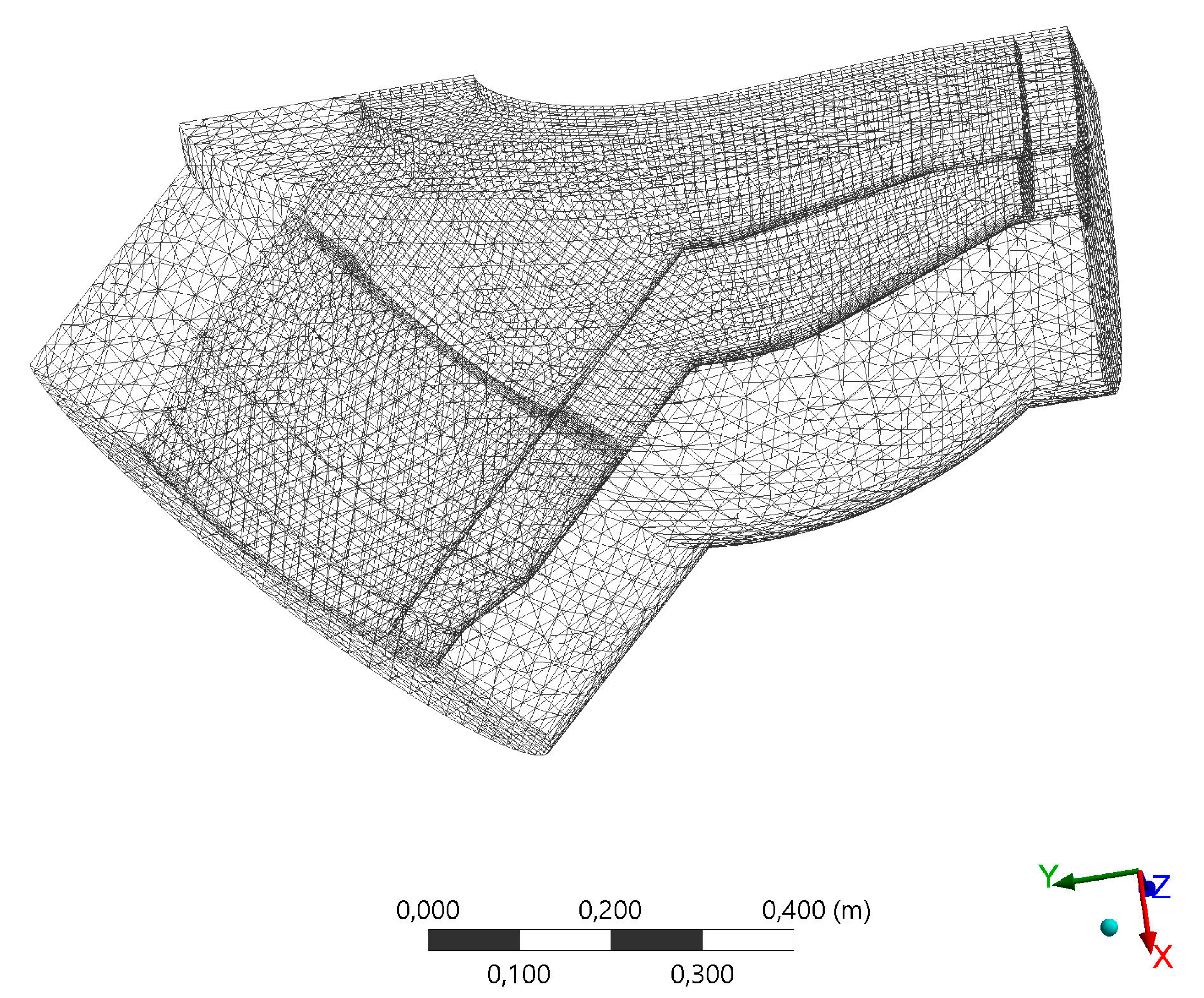
With respect to vertical symmetry planes, a FEM model of a quarter of the junction was created by performing mental sections with the planes of symmetry. A zero value of heat flux was assumed for these planes.

A quarter-section model of the Y-shaped junction was divided into 105 thousand solid finite elements. In the calculations of stress distributions in the symmetry planes, limitations of linear displacements in directions perpendicular to them were assumed. For plane ₁, limited displacements along the pipeline axis, perpendicular to plane ₁, were assumed. Convective heat transfer on the inner surface of the junction between the fluid flowing through the pipeline and the material of the component under consideration was assumed. The heat exchange conditions at the startup and shutdown stages were assumed to be time-dependent. This phenomenon is related to changes in flow rates and steam parameters, for which the heat transfer coefficient of the pipeline may vary depending on the values of the temperature, pressure, the flow type and rate and the geometry of the tested component.

4. The Influence of the Approach to Heat Exchange Phenomena on the Time-Varying Temperature Fields in the Y-Shaped Junction, as Determined by the Application of FEM

The model described in the previous chapter enabled the determination of time-varying temperature fields for various boundary conditions determining the heat transfer on the inner surface of the Y-shaped junction. Papers [10,11,22,23] presented a numerical study of the impact of varying heat transfer conditions on the stress and strain fields on a thick-walled component of a power boiler. This would indicate that operation periods with transient values of the coefficient should be studied thoroughly, and the determination of the coefficient is crucial with regard to the sought-for stress and strain conditions inside a thick-walled power boiler component.

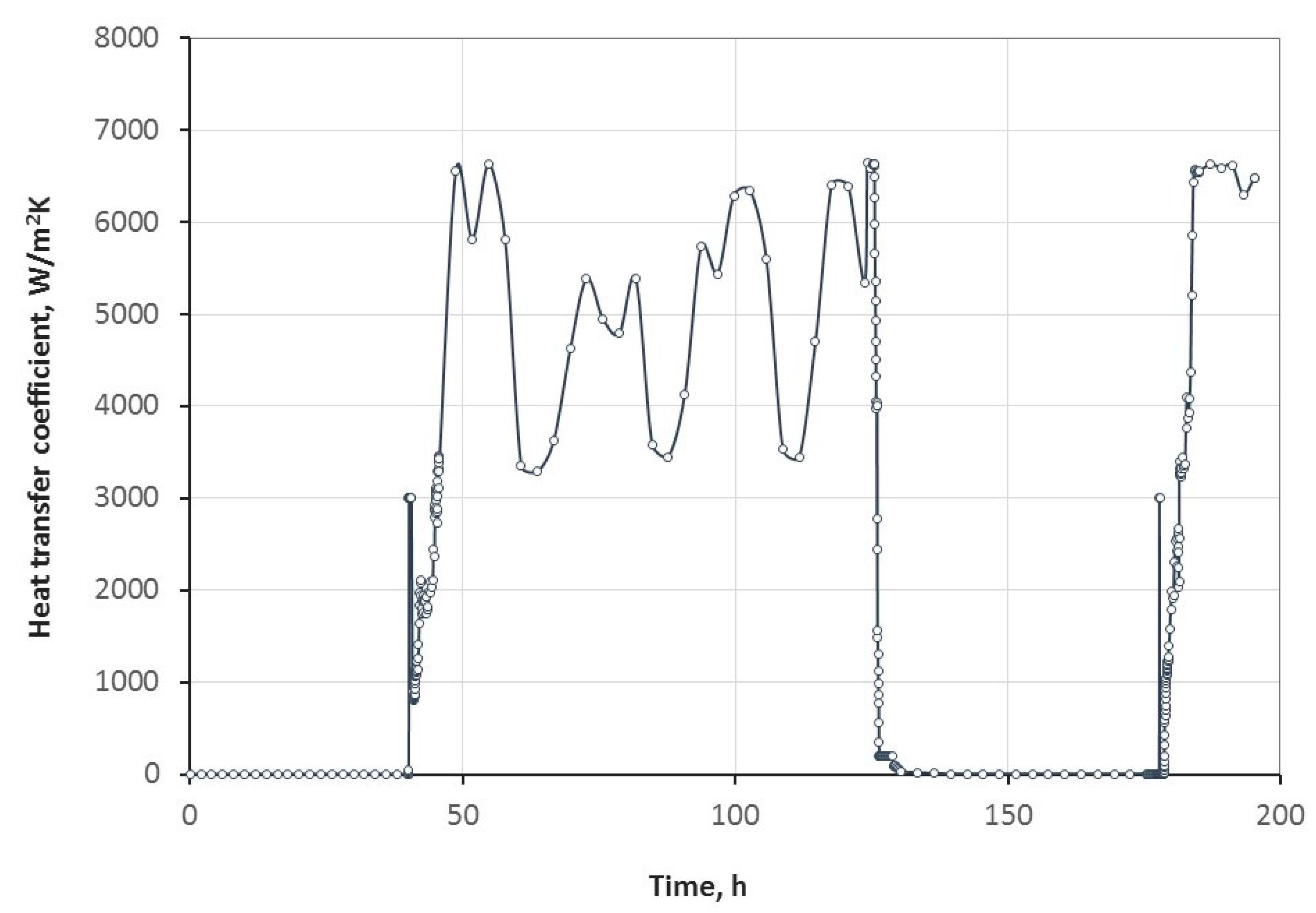
The method of determining the time-varying heat transfer coefficient in models of thick-walled pressure vessels of power engineering devices has been presented in the paper. The applied method is based on heat transfer correlations for turbulent tube flow, including the Nusselt number, and on matching the characteristics of this variable to the measured temperature in the volume of the elements under consideration. For this purpose, available data of measurements performed under industrial conditions were employed.

The analysis was conducted for constant and time-varying heat transfer coefficients with the assumption that the adopted coefficients are independent of the location of the point on the considered surface. In the first approximation, the assumed value of the coefficient was that suggested by the standards used in the power industry in the process of designing high-pressure and temperature vessels [4]. For steam, this coefficient equals 1000 W/m²K. Assuming that heat exchange between the steam and the material on the inner surface of the junction takes place by means of convection and that the heat exchange between the outer surface of the insulation and the immediate surroundings proceeds in a similar way, the time-varying temperature field in the Y-junction was determined. Subsequently, temperature values determined in the FEM simulations for selected points located shallow and deep under the inner surface of the junction were compared with those obtained under operating conditions. 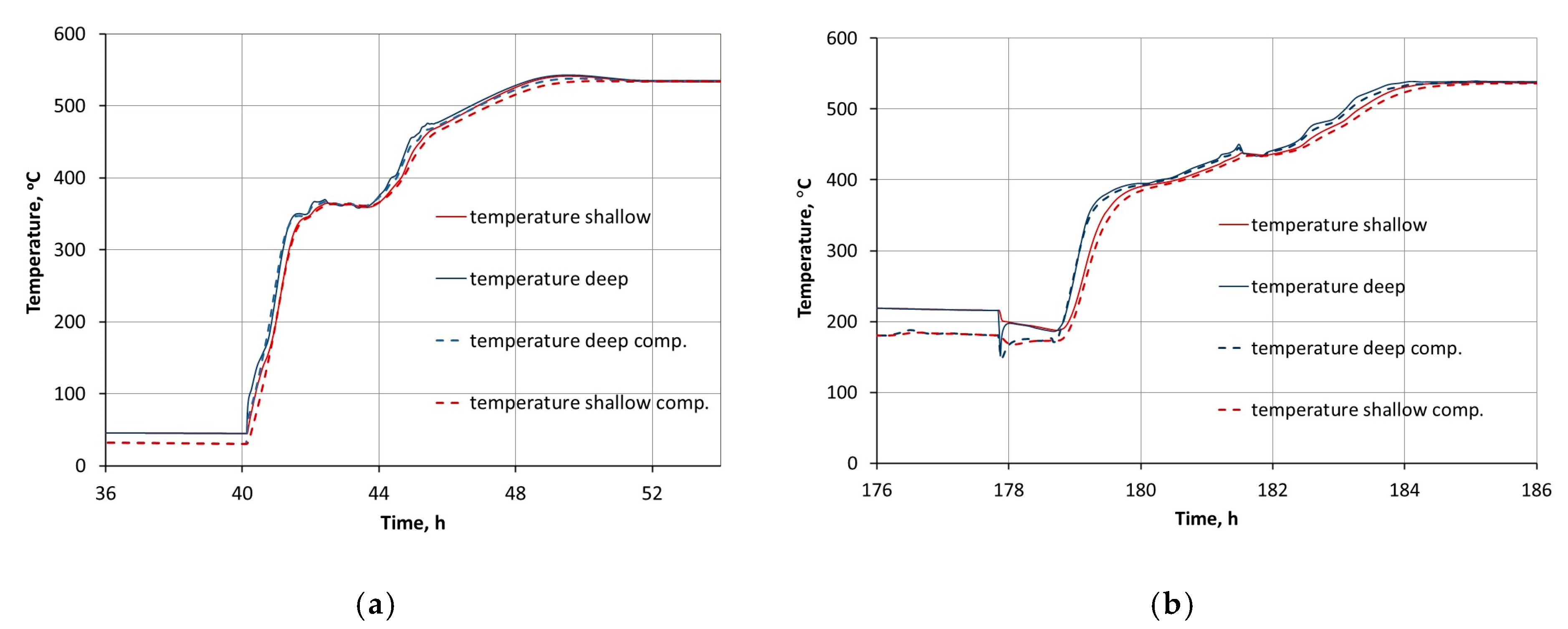Figure 8 shows a comparison of the characteristics of temperature changes at the above-mentioned points for specific time intervals at the startups of the pipeline from cold and hot states, in which temperatures increase rapidly.

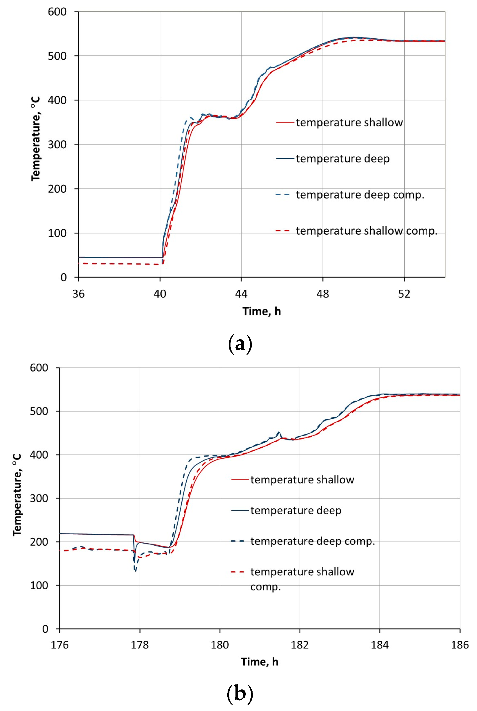
Similar calculations were made for the heat transfer coefficient of 3000 W/m²K. The results and comparison with the results of measurements are shown in Figure 9.

The calculations performed show significant discrepancies between the values determined with the FEM software and those measured with thermocouples. These differences are especially evident at the initial stage of each of the startups (Figure 8 and Figure 9). The discrepancies observed will have a significant impact on the accuracy of the estimations of the time-varying thermal stresses caused by uneven temperature fields in the Y-shaped junction.

In order to achieve better compatibility between the experimental and numerical results, the subsequent calculations assumed that the heat transfer coefficient depends on characteristic numbers, which can be determined on the basis of the parameters of steam flow through the pipeline. The limitations of this method lie in (i) the range of Reynolds Re and Prandtl Pr numbers, for which characteristic equations were developed, (ii) the shape of the tested channel, and (iii) the inclusion or non-inclusion of the direction of heat flow was in the study. Reynolds number ranges depend on the patterns of the flow, i.e., whether the flow is laminar or turbulent. Parameters required for the application of characteristic equations include flow quantities, i.e., flow velocity or mass flow rate, and the physical properties of the medium: its temperature, pressure, dynamic viscosity, density and thermal conductivity. 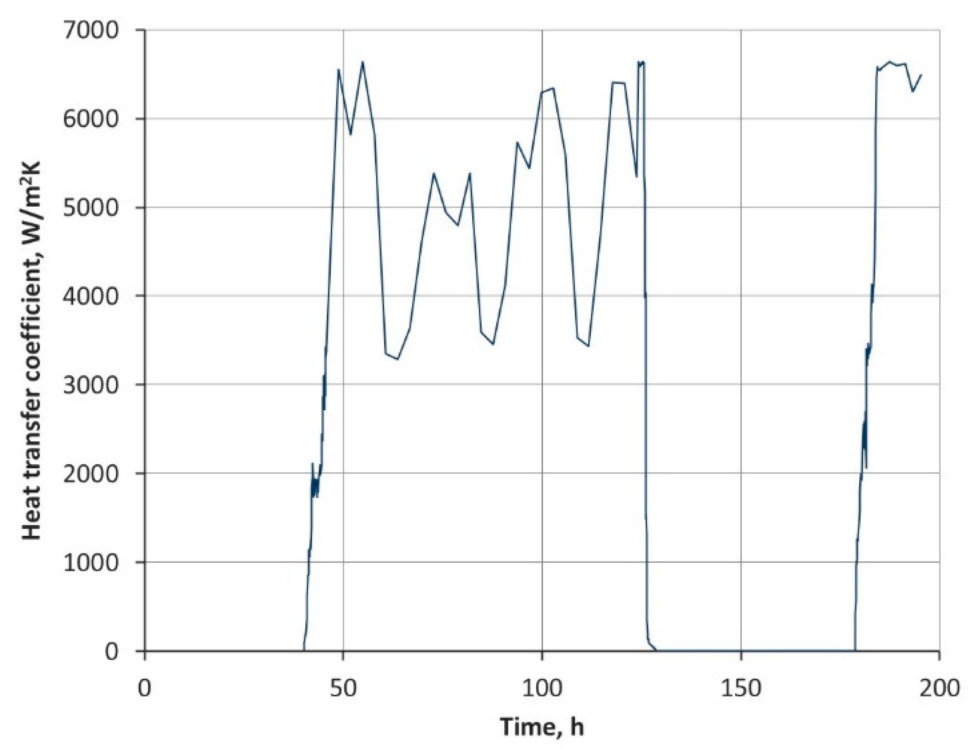On the basis of these values, the time-varying Reynolds number and Prandtl number [24] were calculated, followed by the Nusselt number and the heat transfer coefficient based on the latter. Changes in the time function of thus determining coefficient for a pipe with an internal diameter equal to that of the spherical part of the Y-junction are shown in Figure 10. The characteristics shown in Figure 10 were then taken into account in the calculations of temperature fields, with the assumption that coefficient α on the inner surface of the junction changes in accordance with the relationship shown in this figure and remains constant on the outer surface of the insulation at 10 W/m²K.

Figure 11 compares the results of calculations with measurements taken under operating conditions. These characteristics show large discrepancies between the predicted results and the actual values. This applies, in particular, to the initial stage of the startup period, which is less than 1 h for both startups. As can be seen in Figure 11, the calculated temperatures for deep and shallow points are lower than those measured under operating conditions, yet their differences are similar in the initial stage of the cold startup, which would suggest the adoption of an underestimated value of in calculation. Since values of temperatures are determined by the supplied heat flux, which depends on, but the temperature gradient of the material is determined by its thermal conductivity. However, it can be noticed that with some of the characteristics corresponding to lower heating rates and in the range of the boiler’s steady-state operation, the application of a method for determining the value of the heat transfer coefficient, based on the use of characteristic numbers, yields computational data which are consistent with the results of measurements under industrial conditions.

It could, therefore, be concluded that the heat exchange process at the initial stage of the startups was caused by phenomena other than those that occur at a steady medium flow in the pipeline. Since major discrepancies occur at the initial phases of the startups, when the pipeline inside, the temperature of which is equal to the air temperature—for the cold state it is approximately 30°C, and for the hot state it is approximately 200°C, and the pressure is 0.1 MPa. At the above-mentioned pressure and temperature values, water changes in physical states, i.e., both liquid and vapor states, are likely to occur over this short period of time. Until now, this process, taking place in the time intervals of unsteady operation of the boiler, has not been described in a way that would enable the development of a method for assessing the related heat exchange phenomena. Therefore, in this study, the determination of coefficient α in these particular intervals was based on a method of matching the assumed dependencies of time-dependent coefficient α to the response of the model in the form of temperature–time dependence for the considered measurement points in the Y-junction.

A number of modifications of the characteristics presented in Figure 9 were considered. A correction was made for narrow time intervals at the very beginning of both analyzed startups. For instance, a correction of the heat transfer coefficient, by adopting its value at 1000 W/m²K, i.e., as for steam in the standard [4], and 3000 W/m²K, as for water in the same standard, was considered. One of the relevant characteristics is shown in Figure 12.

The graphs obtained on the basis of calculations of temperature changes as a function of time, with the assumed characteristics of changes in coefficient α (Figure 12) are shown with dashed lines in Figure 13.

The curves from calculation and measurements in Figure 13 do not differ significantly. The differences primarily concern the minimum temperature values at the beginning of the hot startup. There are, however, significant differences between these graphs and the characteristics shown in Figure 8 and Figure 10. Based on these considerations of the cases shown in Figure 8, Figure 10, Figure 11 and Figure 13, it can be concluded that the best correspondence between the calculation results and the test results was achieved for the characteristics of changes in the heat transfer coefficient as shown in Figure 12.

Therefore, it is possible to map the course of changes in temperature distributions in the component under analysis on the basis of a model approach using the FEM with an appropriate selection of time-varying heat transfer coefficients. For cases like the one described in this paper, methods based on the use of characteristic numbers, combined with local modifications of the values of the coefficient at the moments of unstable changes in the steam parameters at the beginning of each boiler startup, could be the basis for the estimation of the characteristics of time-varying heat transfer coefficients.

5. Stress–Strain Behavior of Y-Shaped Junction Induced by Variable Temperature Field and Pressure

The determined temperature field enabled calculations of the variable stress field in the component. The calculations were made for two selected cases (Figure 8 and Figure 13). One included computational results obtained for the assumed constant value of the heat transfer coefficient, equal to 1000 W/m²K as determined in the standards. 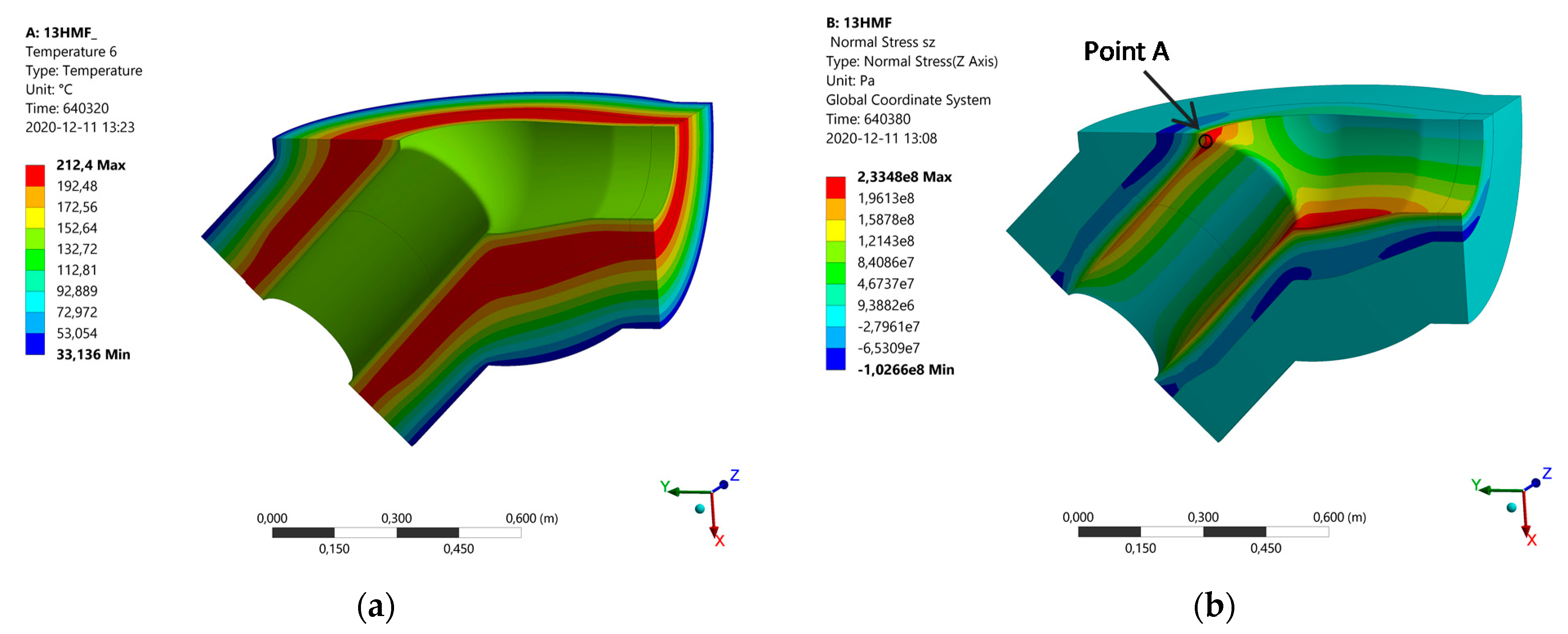The other case was the results of calculations performed for α determined on the basis of the Nu number with a local modification, 3000 W/m²K, for which the best correspondence of the computational results and local measurements of the temperature field was obtained. For a comparison of the results, an area was selected with the highest equivalent stresses, calculated according to the Huber–Mises hypothesis, on the inner surface of the junction (Figure 14).

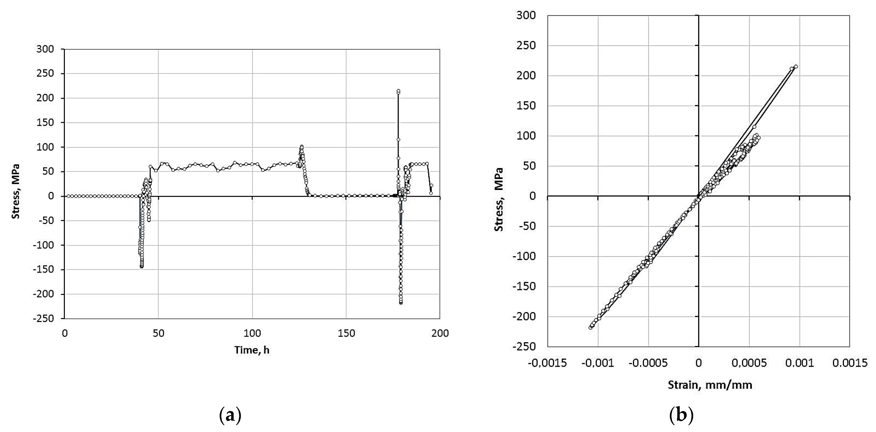
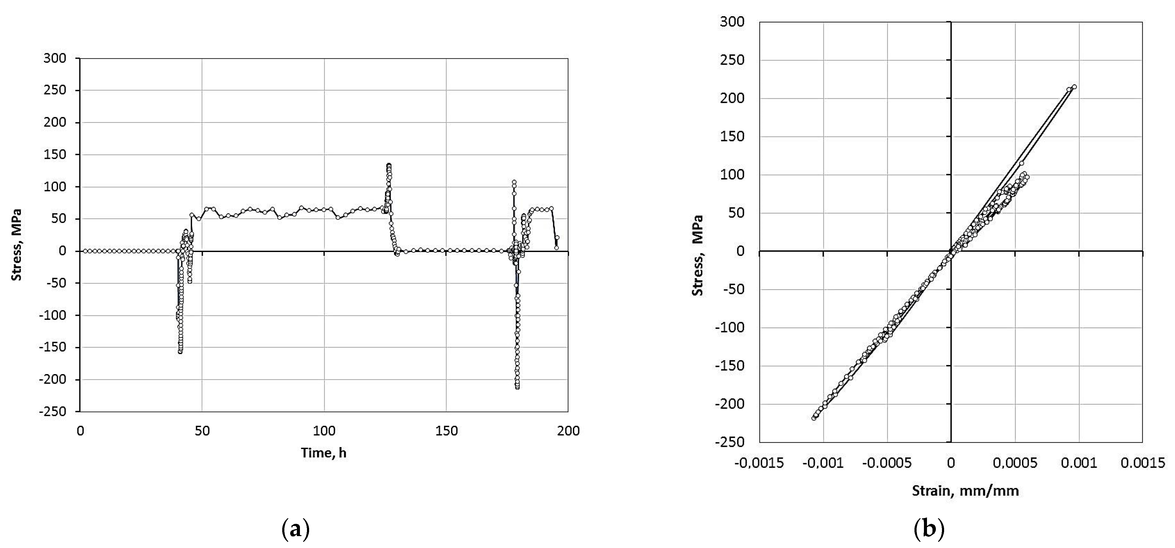
The courses of changes in stress components for both considered cases at the same selected point in this area were determined. The highest values of the determined stress components in the junction occurred in the same short time intervals of rapid temperature changes (Figure 15 and Figure 16), i.e., in the intervals between 640,320 s and 640,380 s, and between 144,480 s and 146,100 s.

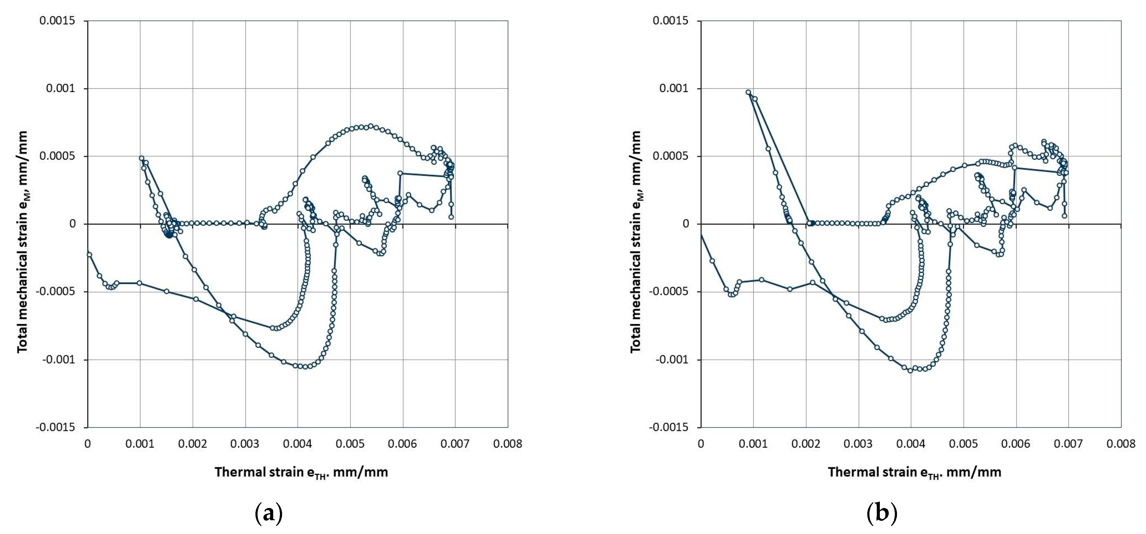
The local dependencies between mechanical and thermal strains were calculated for point A (Figure 14) as well—Figure 17. Such dependencies in the problems of thermomechanical fatigue (TMF) testing characterize the type of fatigue test used. The most common TMF tests are for which the mechanical strain is in phase with thermal strain, and tests in which the course of changes in the time of mechanical strain is shifted in relation to the thermal strain by a time equals to half the period of the thermal-loading cycle [25,26,27,28]. The local characteristics of the relationship between mechanical and thermal strains calculated for real working conditions, shown in Figure 17, are of a much more complex nature. On their basis, it can be seen that both the maximum and the changing range of this mechanical strain, which are often the fatigue life criteria, show higher values for the characteristics shown in Figure 17. Therefore, it should be expected that the durability prediction based on the values of fatigue parameters estimated using the method presented in the paper would give more conservative results compared to the estimation based on the use of a constant heat transfer coefficient.

It can be concluded that the time-varying stress values in the areas with the highest equivalent stresses, caused by the uneven temperature field in intervals of rapid temperature changes, are mainly responsible for the strength and durability of the component under consideration. Such intervals were recorded during both cold and hot startups. It can also be noticed that for the case for which the best consistency of the results of calculations and temperature measurements was obtained, the stresses at the point adopted as characteristic are higher than those calculated for the boundary condition assuming heat exchange based on coefficient α = 1000 W/m²K recommended in the standards. Taking into account both an improved consistency of the calculation results for the temperature field with the measurement results as well as the applicability of a more conservative approach to the analysis of the stress fields from the point of view of the strength and durability of the component under consideration, the following part of this study reports on a detailed analysis of the model of the Y-junction, for which the heat exchange on the inner surface was determined with heat transfer based on characteristic numbers with local modifications, assuming its increase at the beginning of each startup up to 3000 W/m²K.

When considering this case, it can be noted that at the beginning of the cold startup, the difference between the internal and external surface temperatures at the initial phase of the startup has a positive sign. In the other case, the hot startup, this difference takes a negative value. The consequence of such changes in the temperature field includes high values of compressive stresses at the initial phase of the cold startup, while in the hot startup conditions, high tensile stresses occur at the initial stage. Thus, taking into account the nature of the processes of crack formation and growth in components subjected to variable stresses, tensile stress should be considered more dangerous. Large numerical values of stress in hot start conditions seem to be more threatening considering the risk of crack formation caused by successive shutdowns and startups of the installation.

6. Conclusions

This study analyzes the temperature field and stresses in a selected component of a power installation, with a focus on the probability of damage induced by changes in temperature fields and the accompanying thermal stresses. The considerations were based on available data obtained from measurements performed under industrial conditions. The results obtained enable the formulation of conclusions relating to both this individual case of the analyzed element as well as general conclusions concerning the methods of mechanical behavior analysis for elements subjected to complex mechanical and thermal loads, including the method of determining (i) the critical—in terms of strength and durability—working time intervals, in which the parameters responsible for the development of damage reach their highest values and, above all, (ii) guidelines for methods of strength analysis in component parts of conventional energy devices. The operating conditions of these devices will need to change due to the necessity of the coexistence of conventional energy and renewable energy installations.

The new conditions for the operation of fossil-fuel power plants will result in the necessity of frequent startups and shutdowns of installations related to the need to adapt them to the current varying demand for power. Hence, the role of the transition periods during operation will become more important. Therefore, the importance of the awareness of the impact of these periods on stability, operational safety and durability will increase. This study is an attempt at a methodical approach to the strength analysis process of a component in a power-generating installation, for which thermal stresses caused by transient states are of particular importance, and to formulate more general conclusions regarding the impact of operating conditions of conventional energy installations on their durability.

The issue discussed is one of the elements of the methodology for assessing the durability of elements subjected to complex mechanical and thermal interactions, for which thermomechanical fatigue processes play an important role [5,6,25,26,27,28]. The analysis of failure occurrence under such fatigue processes is particularly complex due to the unfeasibility of direct measurement of thermal interactions, as well as the complex methodology for the assessment of material properties. At the present stage, the focus is on the issue of assessing the magnitude of the impacts caused by a variable, nonuniform temperature field in complex-shaped components of energy devices. A selected example of an element operating in a power boiler installation was used.

More detailed conclusions appear in the following chapters, which discuss the results of the performed measurements and calculations; therefore, an attempt is made here to formulate broad conclusions:

• The measurements performed and the FEM computations showed the need for a detailed analysis of the states of transient operation of conventional power devices under new operating conditions related to the use of renewable energy sources in order to determine the conditions which may compromise the safety of operation;
• The model approach to the application of thick-walled elements in these devices, particularly those exposed to damage, enables the determination of both locations and time periods during their operation, in which the process of damage is the most intense;
• One of the key problems in determining the accuracy of the model mapping of the working conditions of thick-walled power installations is the description of the time-varying characteristics of the heat transfer coefficient, which depend on the parameters of the medium inside the installation;
• The application of simple solutions that consist of matching calculated the model’s response in the form of temperature–time dependencies to the recorded at selected points in the analyzed component seems to be sufficiently accurate for the initial stage of the analysis.