A Quantification Method for Supraharmonic Emissions Based on Outlier Detection Algorithms

Abstract

Based on outlier detection algorithms, a feasible quantification method for supraharmonic emission signals is presented. It is designed to tackle the requirements of high-resolution and low data volume simultaneously in the frequency domain. The proposed method was developed from the skewed distribution data model and the self-tuning parameters of density-based spatial clustering of applications with noise (DBSCAN) algorithm. Specifically, the data distribution of the supraharmonic band was analyzed first by the Jarque–Bera test. The threshold was determined based on the distribution model to filter out noise. Subsequently, the DBSCAN clustering algorithm parameters were adjusted automatically, according to the k-dist curve slope variation and the dichotomy parameter seeking algorithm, followed by the clustering. The supraharmonic emission points were analyzed as outliers. Finally, simulated and experimental data were applied to verify the effectiveness of the proposed method. On the basis of the detection results, a spectrum with the same resolution as the original spectrum was obtained. The amount of data declined by more than three orders of magnitude compared to the original spectrum. The presented method will benefit the analysis of quantification for the amplitude and frequency of supraharmonic emissions.

1. Introduction

Due to the fact that power electronic devices are widely deployed in the power grid, in addition to the low-frequency harmonic emissions, the phenomenon of supraharmonic emissions in the frequency range 2 kHz–150 kHz has also been observed [1,2,3]. There is a relatively complete system for the low-order harmonic quantification method and evaluation criteria. More concerns have been turned to the emissions in the supraharmonic frequency band. At present including generation mechanism, propagation mode, and interactive influence, various researches on supraharmonics have been discussed [4,5]. Precise measurement of supraharmonics is the premise of the above analysis.

Currently, there is still no unified standard for measurement methods, EMC level, and immunity level in 2–150 kHz [6]. International standards such as the European Standards (EN) 50,160 and the International Electrical Commission (IEC) 61000-4-19 have discussed emissions higher than 2 kHz. The International Special Committee on Radio Interference (CISPR) 16-2-1 discusses an immunity test method for high-frequency harmonics caused by intentional emissions with a range of 9–30 MHz [7]. The following two guiding methods are mainly recommended regarding the measurement methods of supraharmonics caused by unintentional emissions. Method A is based on the method of 2–9 kHz in Appendix B of IEC 61000-4-7 [8], a fixed rectangular window of 200 ms is selected as a sampling interval, and the application range of the 200 Hz bandwidth grouping is extended to 2–150 kHz. All the tested data are used, which is a gapless treatment approach. In method B, the 32-segment 0.5 ms equal interval sampling method is provided in Appendix C of IEC 61000-4-30 [9], resulting in the resolution of 2 kHz. Since only a 16 ms time window in ten fundamental cycles of 50 Hz power frequency is sampled in this method, the amount of sampled data is significantly reduced compared to method A. Nevertheless, only 8% of the total measured data are applied by method B, which affects the accuracy of the measurement results.

To improve the accuracy of the frequency and amplitude of the measurement results, some scholars have investigated this issue from the perspective of the frequency domain. In [10], a variable bandwidth grouping method was introduced based on the switching frequency. Compared with the fixed 200 Hz bandwidth, this method could reflect the amplitude and frequency of supraharmonics more accurately. However, it is difficult to accurately identify the respective switching frequencies when multiple different emission sources are presented. Moreover, the authors in [11] provided a new method based on multiple measurement vectors model and orthogonal matching algorithm, designed to increase the frequency domain resolution from 2000 Hz to 200 Hz without increasing the observation duration. However, this method requires a priori knowledge of signal sparsity. In [12], a method for quantization supraharmonics based on wavelet decomposition was proposed. This method can achieve the same level of resolution as IEC 61000-4-7, but wavelet packet coefficients will be affected by signal time deviation.

To further explore the approaches to supraharmonic quantification, some studies have attempted to reduce the amount of sampled data from the perspective of time sampling. For example, in the method presented in [13], the filter banks and compressive sampling reduced the sampling frequency without changing the performance of existing measuring equipment, but the amplitude and phase angle of the narrowband signals will be affected by the analog filter bank. In [14], a polyphase discrete Fourier transform (DFT) filter bank was implemented to handle data in the 2–150 kHz frequency band. Compared with method B, this method has fewer operations and stronger robustness. However, this method is still limited by the frequency domain resolution of 2000 Hz.

The above approaches are designed to quantify supraharmonic emission results more effectively. However, due to the mutual restriction between the resolution and the amount of data in the frequency domain, it is challenging to simultaneously meet the demand for low data storage and high resolution. In particular, the supraharmonic frequency points generated by the pulse width modulation of power electronic converter devices are distributed at m f_c ± n f_s, where f_c is the carrier wave frequency (switching frequency), and f_s is the fundamental frequency, and m and n are the carrier wave and modulation wave order, respectively [15]. The emissions of supraharmonics were up to 150 kHz and accompanied by sideband emissions. As such, it requires a more accurate evaluation of the supraharmonic emissions.

The supraharmonic frequency band is characterized by many low-amplitude noise points and few higher-amplitude supraharmonic emission signals. Based on the difference in the density distribution of noise and emission points, supraharmonic emissions can be regarded as outliers to analyze. At present, outlier detection technology has been widely used in financial fraud, fault monitoring, and other fields [16]. The outliers deviate significantly from other observations, and some data analysis techniques choose to discard these obviously different points. However, in some scenarios, the outliers may be caused by a specific type of mechanism. Potential and meaningful information may also be present in these points. This paper focused on the analysis of outliers in the frequency range of 2–150 kHz.

The mean and standard deviation method based on normal distribution is commonly used to detect outliers, but this method is easily affected by extreme values. Due to the existence of supraharmonic components, the data usually exhibits skewed distribution characteristics. Further research has also verified that the standard normal distribution is unsuitable for describing the 2–150 kHz data distribution [17]. The influence of outliers on the supraharmonic range is discussed in detail in Section 3.1. In this paper, an appropriate threshold was selected according to the data distribution model, and the noise points below the threshold were filtered out.

However, there is still residual noise from the previous steps, so the clustering algorithm was further used to extract the supraharmonic components more accurately. The clustering-based DBSCAN algorithm does not need to specify the number of clusters in advance. Besides, the algorithm can identify the arbitrary shape of data clusters and can also handle outliers efficiently. Therefore, the DBSCAN algorithm was selected for clustering analysis.

The clustering effect of DBSCAN is determined by the minimum number of points (MinPts) and epsilon (Eps). In order to obtain the best clustering effect, the author determined the MinPts and Eps by binary differential evolution algorithm in [18]. The grid division technology in [19] and the multi-verse optimizer algorithm in [20] were also strategies to determine DBSCAN parameters. In addition, the multi-objective genetic algorithm was applied to find the optimal solution of the clustering parameters in [21]. Nevertheless, the above algorithm implementation steps are more complicated. To realize the automatic tuning of DBSCAN parameters, a feasible and straightforward method is proposed in this paper, based on the slope set of the k-dist curve and the dichotomy.

The DBSCAN algorithm handles the neighborhood of all core points. In the absence of any preprocessing, excessive data will result in limitations of operational efficiency. Before the DBSCAN algorithm is executed, the amount of data can be filtered out by removing the noise below the threshold of the data distribution model. For the above reasons, the skewed distribution model and the DBSCAN algorithm were combined in this paper as a tool for supraharmonic emissions quantification, denoted as the SD-DBSCAN method.

The main contributions of this research are as follows:

• On the basis of the outlier characteristics of supraharmonic emissions, outlier detection algorithms can be employed to quantify the supraharmonic emission signals;
• Based on the data distribution of slope point set and dichotomy, a self-tuning DBSCAN algorithm is presented. Additionally, a new method that combines the skewed distribution model and the self-tuning parameter DBSCAN clustering algorithm (SD-DBSCAN) is introduced in detail.
• The newly proposed method solves the contradiction between the data volume of results and the frequency domain resolution. It has the advantage of a high resolution in the frequency domain.

The rest of the paper is structured as follows. Section 2 describes the principle of the SD-DBSCAN method and the implementation steps in detail. In Section 3, the method is verified by means of simulated and real signals. A systematic discussion and analysis of the different methods are presented in Section 4. Finally, the conclusions are shown in Section 5.

2. Description of the SD-DBSCAN Method

In this section, the implementation procedure of the SD-DBSCAN method is explained in detail and can mainly be divided into three parts. The first part is the analysis of the data distribution model based on statistics; the second part is the principle of the DBSCAN algorithm and the automatic tuning of its parameters; and the last part introduces the specific steps of SD-DBSCAN and the evaluation metrics.

2.1. Statistics-Based Outlier Detection

Based on statistics, the points with low probability density distribution are regarded as outliers. The probability density distribution is usually described by the Jarque–Bera test, based on the sample skewness and kurtosis [22]. Skewness and kurtosis reflect the asymmetry and the sharpness of the overall distribution density function, respectively. For random variables {X_i}_i=1,p, p represents the number of samples, and the definitions of skewness β₁ and kurtosis β₂ are expressed as Equations (1) and (2). The Jarque–Bera test statistic is given by Equation (3):

$${\beta }_1=\frac{1}{p}{\displaystyle \sum _{i=1}^p{(X_i-\overline{X})}^3/{\left(\frac{1}{p}{\displaystyle \sum _{i=1}^p{(X_i-\overline{X})}^2}\right)}^{3/2}},$$

(1)

$${\beta }_2=\frac{1}{p}{\displaystyle \sum _{i=1}^p{(X_i-\overline{X})}^4/{\left(\frac{1}{p}{\displaystyle \sum _{i=1}^p{(X_i-\overline{X})}^2}\right)}^2},$$

(2)

$$JB=\frac{p}{6}\left[{\beta }_1^2+\frac{{({\beta }_2-3)}^2}{4}\right],$$

(3)

where $\overline{X}=\left(1/p\right){\displaystyle \sum }_{i=1}^p{X}_i$; and JB represents the calculation result of the Jarque–Bera test. Under a normal distribution condition, the test results follow the chi-square distribution ($\chi$²) with degrees of freedom of 2, giving the significance level α = 0.05 and the critical value of ${\chi }_{1-\alpha ,2}^2$ [23]. If the Jarque–Bera test statistic is less than the critical value, it will obey the normal distribution. Otherwise, it belongs to the right/left-skewed distribution according to the positive or negative value of skewness.

For skewed distribution data, it is appropriate to use the median to reflect the centralized trend. The absolute median deviation (MAD) expresses the discrete trend. In the statistical analysis of geochemistry data, median and MAD are widely used [24]. They overcome the limitation of non-normal distribution and have strong robustness to skewed distribution data. If the data in the supraharmonic frequency band meets the normal distribution, the corresponding outlier threshold is the sum of the mean and two times the standard deviation (mean + 2SD). If the frequency band belongs to the skewed distribution, the outlier detection threshold is the median + 2MAD [25]. The MAD calculation formula is shown in Equation (4):

$$\mathrm{MAD}=median\left(\left|X_i-median(X)\right|\right).$$

(4)

Since the above method can only dispose of the noise below the threshold preliminarily, there are remaining noise components. Further clustering analysis is essential.

2.2. DBSCAN Algorithm

For the DBSCAN algorithm, if the number of points in the Eps range of a certain point exceeds MinPts, a cluster with that point as the core will be created. All points within the Eps range of the core point are considered part of this cluster (direct density-reachable objects). If any point in the cluster is also identified as a new core point, the points within the Eps range of this new core point are included in this cluster transitively (density-reachable objects). Then, DBSCAN iteratively finds the direct density-reachable and density-reachable objects from the core object. Points that do not belong to any cluster are considered outliers [26]. The key to the algorithm is how to determine MinPts and Eps adaptively. In this paper, a method for automatically determining the MinPts and Eps was implemented based on the dichotomy.

2.2.1. Determine the Eps

The distance distribution matrix of the input dataset was calculated to obtain a k-dist diagram, and k is the column subscript of the matrix. The distance measurement method adopts the Euclidean calculation formula. The slope variation of each point on the k-dist curve is applied to select the Eps parameter. Assuming that the slope of point i is d(i), and the calculation formula is expressed in Equation (5):

$$d(i)=|k\_dist(i)-k\_dist(i+1)|.$$

(5)

If the optimal MinPts = k, Eps_k represents the epsilon at the optimal value of k, the steps for self-tuning Eps_k are as follows:

• The slope of each point is calculated according to Equation (5), and the point where the slope is zero is removed to obtain the slope set;
• The skewness, kurtosis, and the Jarque–Bera test statistic of the slope set is calculated based on Equations (1)–(3), then the probability distribution is further presented;
• If the slope set belongs to the normal distribution, the first point greater than mean + 2SD is found. The distance value corresponding to this point is regarded as the Eps_k. If the new dataset belongs to skewed distribution, the distance value corresponding to the first point greater than median + 2MAD is taken as the Eps_k.

2.2.2. Determine the MinPts

The primary route for determining the optimal MinPts is as follows: multiple sets of Minpts and Eps parameters are used as the input of the clustering algorithm, and the number of clusters is output, denoted by C in the following discussion. When the value of C is stable for three consecutive times, the optimal number of clusters is obtained, represented by Opc. When the output C equals Opc, the minimum value of k is taken as the optimal MinPts.

For a two-dimensional array, the MinPts should be greater than or equal to 2. However, if the MinPts is too large, the corresponding Eps will be larger, resulting in all points being classified into one category. For a large capacity dataset, the clustering results have entered a stable state when MinPts is taken as the integer closest to N/25 [27]. Thus, when MinPts = k, k_min = 2 and k_max = N/25 (round to the nearest integer). Within the range of k_min to k_max, the dichotomy is utilized to determine the minimum value of k when the output C is equal to Opc. This is a simple and effective optimization algorithm for seeking parameters, l is the index counter, and C_l represents the number of clusters of the l-th DBSCAN clustering. The specific procedure of the seeking algorithm is shown in Figure 1.

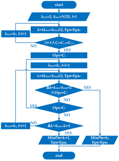
Figure 1. The procedure of parameter seeking based on the dichotomy, where k is rounded to the nearest integer.

Through the above steps, the optimal Eps and MinPts can be determined adaptively.

2.3. Method Structure

2.3.1. Flow Chart

The implementation of the SD-DBSCAN method proposed in this paper can be divided into the following six steps, as described in Figure 2.

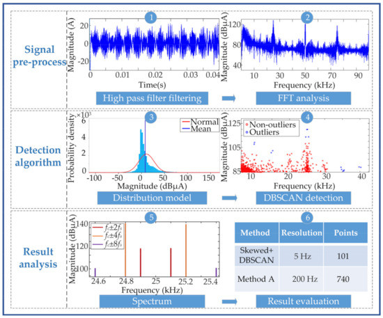
Figure 2. The flow chart of the proposed SD-DBSCAN method.

Step 1–Step 2: Data pre-processing.

An Elliptic digital filter was designed to filter the harmonics with frequencies below 2 kHz, and then the Fourier transform was applied to the filtered signals. For the sake of distinction, this dataset after Fourier transform is represented by X.

Step 3: Determine the probability distribution model and extract the new dataset.

Utilize the Jarque–Bera test to obtain the probability distribution model of dataset X. The detection threshold was set according to the corresponding distribution model, then points larger than the threshold can be extracted to compose dataset Y.

Step 4: Adaptively determine the parameters of DBSCAN and then perform DBSCAN clustering.

Since different dimensions may lead to unreasonable results, standardization is included before clustering. Thus, the matrix Y is standardized, and then the distance distribution matrix of the matrix Y is constructed to obtain the k-dist curve when k takes different values. The MinPts and Eps are determined according to the dichotomy parameter seeking algorithm in Section 2.2. Finally, the optimal clustering results are obtained.

Step 5: Generate a spectrum of detect results.

Based on the points detected by DBSCAN clustering, the final spectrum is obtained. The spectral resolution is 5 Hz at a 200 ms sampling window length.

Step 6: Evaluation of detection effect of supraharmonic emission signals.

The signal detection effect was evaluated with reference to the metrics presented in Section 2.3.2.

2.3.2. Performance Metrics

The F-measure index is introduced to verify the effectiveness of the proposed method. Supraharmonic emissions are emitted regularly at switching frequency and its integer multiples, and a priori knowledge about the distribution of supraharmonic signals is a prerequisite for applying this index. F-measure is the weighted harmonic average of recall and precision. The precision is relative to the detection results, and it indicates the number of supraharmonic frequency points among all detected outliers, and the calculation formula is:

$$\mathrm{Precision}=\mathrm{TP}/\left(\mathrm{TP}+\mathrm{FP}\right),$$

(6)

where true positive (TP) represents the true sample is detected as positive, and false positive (FP) represents the false sample is misjudged as positive. The recall illustrates the proportion of detected supraharmonic points to the total supraharmonic points. The false negative (FN) represents the true sample are misjudged as negative, and the recall formula is:

$$\mathrm{Recall}=\mathrm{TP}/\left(\mathrm{TP}+\mathrm{FN}\right).$$

(7)

In order to comprehensively consider the precision and the recall, the indicator F-measure calculation formula is as follows:

$$\mathrm{F}-\mathrm{measure}=2\times \mathrm{Precision}\times \mathrm{Recall}/\left(\mathrm{Precision}+\mathrm{Recall}\right).$$

(8)

F-measure combines the results of recall and precision. The higher the F-measure, the more ideal the clustering effect. Another strategy to evaluate the accuracy of the measurement results is to compare the relative errors of different methods at maximum amplitude [7]. Furthermore, the frequency error corresponding to the maximum amplitude should also be considered. The formula for calculating the relative error of the maximum amplitude (${\delta }_m$) and frequency error (${\Delta }_f$) is shown in Equations (9) and (10).

$${\delta }_m=100\ast \frac{\left|{\max }_{\mathrm{test}}-{\max }_{\mathrm{ref}}\right|}{{\max }_{\mathrm{ref}}},$$

(9)

$${\Delta }_f=\left|f_{\mathrm{test}}-f_{\mathrm{ref}}\right|,$$

(10)

where max_test indicates the maximum amplitude of the test result, and f_test is the frequency corresponding to the max_test. The maximum amplitude and its frequency reference are denoted as max_ref and f_ref, respectively.

3. Results and Analysis

In this section, experimental results of the synthetic and actual signals are given and evaluated. The detection effects of different combined methods are compared.

3.1. Simulation Analysis

In order to verify the proposed method, a set of signals containing supraharmonics superimposed with 20 dB Gaussian white noise was generated using the MATLAB platform. The MATLAB version number used in this work was R2016a, and the filter design and analysis tool (FDATool) toolbox was also used in the high-pass filter design process. The specific frequency points and amplitudes are listed in Table 1, which contains the fundamental component, six supraharmonic components, and one interharmonic component with a frequency of 15,005 Hz. The supraharmonic components use 7550 Hz as the center frequency, and the frequency points of the sideband are spaced at integer multiples of f_s. There are no strict requirements on the signal phase angle.

Table 1. Frequency and magnitude of the synthetic signal.

No.	Frequency (Hz)	Magnitude (A)	No.	Frequency (Hz)	Magnitude (A)
1	50	1.000	5	7700	0.040
2	7400	0.041	6	15,005	0.035
3	7500	0.048	7	15,050	0.023
4	7600	0.050	8	15,150	0.025

The synthetic signal was sampled at a sampling frequency of 1024 kHz to meet the needs of the standard IEC 61000-4-30, and the sampling time window was 200 ms. Figure 3 is the spectrum obtained after filtering out the harmonic frequency below 2 kHz using an elliptical filter.

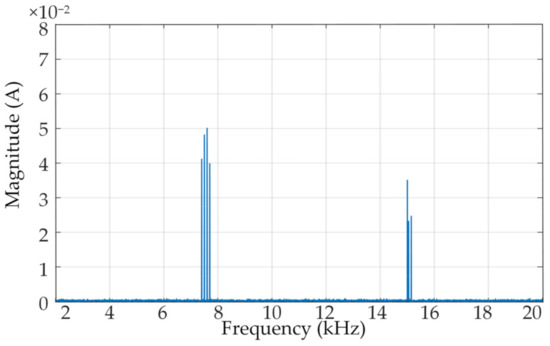
Figure 3. The spectrum of the synthetic signal.

A detailed analysis of data distribution in the supraharmonic band was carried out. The cumulative distribution function (CDF) describes the probability distribution of the variables. The horizontal axis of the quantile–quantile (Q–Q) plot represents the quantiles of the normal distribution, and the vertical axis is the sample quantiles. If a large number of sample points are distributed around the reference line with a slope of one, the sample is normally distributed.

The CDF curve and Q–Q plot in the range of 2–150 kHz without adding the supraharmonic components are shown in Figure 4. The CDF curve of the empirical data is very close to the normal distribution curve. Most of the data points in the Q–Q plot are distributed close to the reference line. After adding the supraharmonic components, the frequency-domain distribution is illustrated in Figure 5. The difference between the empirical data distribution and the normal distribution in Figure 5a is enormous, and most of the empirical data are below 0.5 mA. The distribution of data points in Figure 5b is susceptible to supraharmonic emissions.

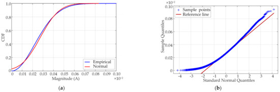
Figure 4. The frequency-domain distribution without supraharmonic signals. (a) Cumulative distribution function (CDF) curve of the normal and empirical distribution; (b) Data distribution quantile–quantile (Q–Q) plot.

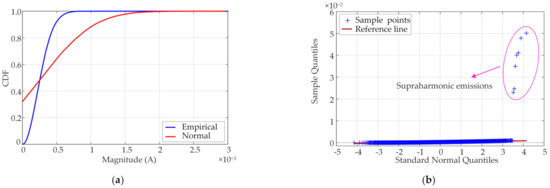
Figure 5. The frequency-domain distribution with supraharmonic signals. (a) CDF curve of the normal distribution and empirical distribution; (b) Data distribution Q–Q plot.

According to Equations (1)–(3), the distribution statistics with and without supraharmonic components were calculated. The thresholds corresponding to the normal distribution and the skewed distribution are listed in Table 2. In addition, since the Tukey algorithm is also an effective method for outlier detection, it is listed in Table 2 for comparison.

Table 2. Signal statistics calculation results.

Statistics	Without Supraharmonics	With Supraharmonics
Skewness	0.6359	64.6769
Kurtosis	3.2696	4606.0511
JB test	≥${\chi }_{1-\alpha ,2}^2$	≥${\chi }_{1-\alpha ,2}^2$
Mean + 2SD	0.00056	0.00150
Median + 2MAD	0.00049	0.00052
Tukey	0.00046	0.00047

The results indicate that in the absence of supraharmonics, the probability distribution of the dataset after filtering by the high-pass filter does not satisfy the standard normal distribution, and the calculated results of skewness and kurtosis are close to the normal distribution. After adding the supraharmonic signals, the kurtosis and skewness of the dataset were far beyond the fitting range of the normal distribution due to the presence of outliers. The skewness of the data points was 64.6769, and the data exhibited an extreme right-skewed and heavily tailed distribution. The kurtosis and skewness of the dataset with the supraharmonic signals were hundreds of times higher than without the supraharmonic signals. The proposed SD-DBSCAN detection method was also developed based on the significant difference in probability distribution with and without supraharmonics. The mean + 2SD threshold was much larger than the median + 2MAD in Table 2. The normal distribution model is unsuitable for accurately fitting the sample data distribution but it is reasonable to apply the skewed distribution model to describe the supraharmonic frequency band distribution.

The Tukey algorithm is also a method with solid robustness for data distribution, but the corresponding detection threshold was the lowest among the three methods. The lower the threshold, the more noise is retained. In contrast, if the threshold is too high, it may cause some valuable points to be filtered out. Selecting the threshold according to the skewed distribution can filter out most of the noise and ensure the retention of valid signals.

In the next stage, DBSCAN clustering was used to further extract the supraharmonic components. The MinPts and Eps need to be determined before clustering. When k takes different values, Eps_k can be determined according to the data distribution of the slope point set of the k-dist curve. Opc is obtained when the number of clusters in the clustering has been stabilized three times. The range of dichotomy is continuously updated until the minimum value of k is found when the output C is equal to Opc.

The results of parameter seeking of the synthetic signal was Minpts = 3 and Eps = 0.0365. The corresponding spectrum of detection results was compared with that of methods A and B, as shown in Figure 6. The signal amplitudes measured by the three measurement methods are listed in Table 3. The detection result of the SD-DBSCAN method is presented as the red spectrum line. Table 4 shows the comparison results of the three methods, which displayed information about the resolution, the maximum amplitude error ${\delta }_m$, frequency error ${\Delta }_f$, the number of result points, and the calculation result of the F-measure index.

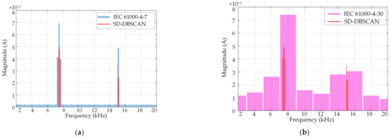
Figure 6. The synthetic signal was analyzed by the proposed method, IEC 61000-4-7 (method A) and IEC 61000-4-30 (method B) in 2–150 kHz. (a) The spectrum of detection results and IEC 61000-4-7. (b) The spectrum of detection results and IEC 61000-4-30.

Table 3. The amplitudes of the synthetic signal measured by the proposed method, IEC 61000-4-7, and IEC 61000-4-30.

Method	7400 Hz	7500 Hz	7600 Hz	7700 Hz	15,005 Hz	15,050 Hz	15,150 Hz
Reference value	0.041	0.048	0.050	0.040	0.035	0.023	0.025
SD-DBSCAN	0.041	0.048	0.050	0.040	0.035	0.023	0.025
IEC 61000-4-7	\	0.069	\	0.039	\	\	\
IEC 61000-4-30	\	\	\	\	\	\	\

Table 4. Results of the synthetic signal processed by the proposed method, IEC 61000-4-7, and IEC 61000-4-30.

Method	${\mathit{\delta }}_{\mathit{m}}$ (%)	${\mathbf{\Delta }}_{\mathit{f}}$ (Hz)	Resolution (Hz)	Result Points	F-Measure
SD-DBSCAN	0	0	5	9	0.87
IEC 61000-4-7	38.68	100	200	740	\
IEC 61000-4-30	46.8	400	2000	74	\

It is noticeable that the amplitude and frequency of the red spectral line in Figure 6 were consistent with the set value. It can also be seen from Table 3 that the proposed method could accurately identify the supraharmonic and interharmonic signals with no error in amplitude with respect to the reference value. The IEC methods cannot accurately reflect the emission points at the corresponding frequencies due to the resolution constraint. Besides, if a fixed grouping bandwidth is selected, there may be a phenomenon with sideband emissions of the same center frequency into other frequency bands. The comparison results in Table 4 also show that the proposed method can achieve the exact resolution as the original spectrum, and the number of result points was the least compared with the IEC method.

Noise with different signal-to-noise ratio (SNR) levels was added to the synthetic signal to test the robustness of the proposed algorithm. The F-measure index was applied to evaluate the detection effect. Figure 7 demonstrates that as the SNR increases, the more significant the difference between the emission signals and noise, and the better the SD-DBSCAN detection effect.

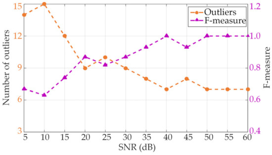
Figure 7. The relationship between SNR, F-measure, and the number of detection outliers.

During the normal operation of the power system, the fluctuation range of the power frequency does not exceed ±0.5 Hz. In order to evaluate the effect of power frequency deviation on the measurement results of different methods, the mean spectral difference (MSD) metric is introduced. The expression for the calculation of the MSD is shown in Equation (11) [12].

$$\mathrm{MSD}=\frac{1}{N}{\displaystyle \sum _{\mathrm{bins}}100}\ast \frac{\left|P_z-Q_z\right|}{Q_z},$$

(11)

where {P_z}_z=1,N denotes the measured spectral at different power frequencies; N denotes the number of frequency bands; and {Q_z}_z=1,N is the reference spectral at 50 Hz power frequency. The MSD of the three methods was analyzed, as given in Figure 8. The higher the value of MSD, the more significant the influence of the power frequency deviation on the measurement results. It can be seen from Figure 8 that the new proposed approach was the least affected by the power frequency deviation.

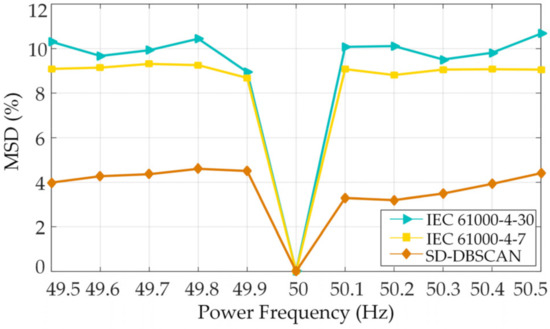
Figure 8. Results of the mean spectral difference (MSD) for different methods at varying power frequencies.

3.2. Measured Analysis

3.2.1. Results Analysis

A LED drive model was also developed as a supraharmonic source to test the newly proposed method. The electrical schematic and test setup are shown in Figure 9, and the relevant parameters are listed in Table 5. The measurement was performed by the ASR-2100 programmable AC/DC power supply to provide input. The Tektronix MDO 3024 oscilloscope with a sampling frequency of 500 kHz was applied to acquire data. A 200 ms sampling interval was employed. The DG1022 function signal generator was used to generate the driving signal of the switching device MOSFET in the LED prototype. The load was a resistor connected in parallel across the capacitor, provided by the IT8511 electronic load. Additionally, the signal was resampled to meet the requirement of method B, equal to 1024 kHz, and then analyzed.

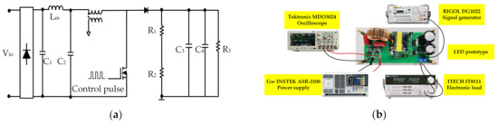
Figure 9. The electrical schematic and test setup. (a) Schematic diagram of the LED driver model. (b) Real test scenario.

Table 5. The circuit parameters of the LED drive model.

Variable	Value
Vin	24 V
C1	1 µF
C2	3.3 µF
Lm	1 mH
C3, C4	470 µF
R1	191 kΩ
R2	1 kΩ
R3	48 Ω
Control pulse	50 kHz

Following the steps described in Section 2.3.1, the threshold was first determined based on the probability distribution model of the filtered dataset X. The CDF curve of the measured data in Figure 10a still deviated significantly from the normal distribution curve. There are obvious outliers in Figure 10b, and dataset X presents evident right-skewed characteristics. The measured kurtosis was 1793.4, and the skewness calculation result was 32.83. The Jarque–Bera test result of dataset X was greater than the critical value, which satisfies the conditions of the skewed distribution model. The median + 2MAD was selected as the upper threshold for preliminary data screening. Furthermore, dataset Y was constituted.

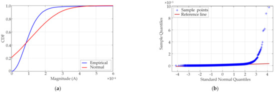
Figure 10. The frequency-domain distribution diagram of the measured signal. (a) CDF distribution curve of the measured signal. (b) Q–Q plot of the measured signal.

Referring to step 4, the matrix Y was first normalized, and then the distance distribution matrix of Y was constructed. The statistical distribution of the k-dist slope set was used to determine the Eps_k. In order to determine the most appropriate value of k, the dichotomy method was adopted to search the parameters. The minimum point where the output C equals Opc was determined to be k = 9 and Eps_k = 0.194. Next, the detection results are given in Figure 11. The data in this figure were divided into two categories, where the red points were identified as non-outliers, and the blue outliers were further analyzed as supraharmonics.

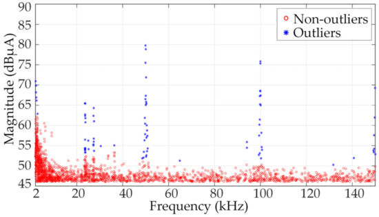
Figure 11. DBSCAN clustering results, points in red were identified as non-outliers, while points in blue were identified as outliers.

In order to verify the validity of the algorithm parameters, Figure 12 shows the variation of k, number of clusters, and the F-measure under different conditions. The number of clusters decreases with the increase in k. Starting from k = 9, the number of clusters enter into a stable state, and the F-measure index was 0.90, proving that the DBSCAN parameter determination method proposed in this work is feasible.

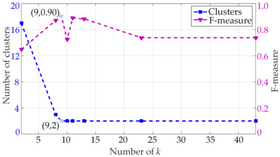
Figure 12. The relationship between the number of k, number of clusters, and the F-measure index with the measured signal.

The spectrum of the clustering results was compared with that of methods A and B, as presented in Figure 13. It can be seen that the amplitudes of the supraharmonics were smaller than that of the ordinary harmonics and the amplitudes decreased with the increase in supraharmonic order. The emissions were concentrated on the switching frequency and its integer multiples. A comparison of the three methods is reported in Table 6, which indicates that the proposed method has superior performance in data storage while ensuring frequency domain resolution. The newly proposed method can capture the frequency of the signal accurately with its excellent resolution characteristics.

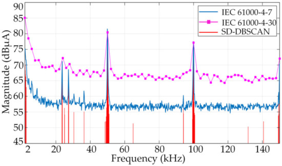
Figure 13. The measured signal was analyzed by the proposed method, IEC 61000-4-7 (method A), and IEC 61000-4-30 (method B).

Table 6. Results of the measured signal processed by the proposed method, IEC 61000-4-7, and IEC 61000-4-30.

Method	${\mathit{\delta }}_{\mathit{m}}$ (%)	${\mathbf{\Delta }}_{\mathit{f}}$ (Hz)	Resolution (Hz)	Results Points	F-Measure
SD-DBSCAN	0	0	5	76	0.90
IEC 61000-4-7	21.57	50	200	740	\
IEC 61000-4-30	7.8	50	2000	74	\

The local spectrograms were analyzed in the 50 kHz and 100 kHz frequency bands to observe the detection results more clearly, as shown in Figure 14. The supraharmonic emissions of the drive model were mainly distributed in the odd-order sideband at the switching frequency and its integer multiples. Emissions of f_c ± 19 f_s could be detected centered at 50 kHz, and emissions of 2 f_c + 15 f_s could be seen centered at 100 kHz.

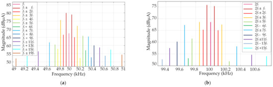
Figure 14. Detailed spectrograms, where f_c is the carrier wave frequency (switching frequency), f_s is the fundamental frequency. (a) Spectrum around 50 kHz. (b) Spectrum around 100 kHz.

3.2.2. Method Comparison

To further evaluate the SD-DBSCAN method, four comparison approaches in Table 7 were employed: method Ⅰ adopted the skewed distribution model and the traditional DBSCAN algorithm; method Ⅱ utilized the normal distribution model and the traditional DBSCAN algorithm; method Ⅲ applied the traditional DBSCAN algorithm to detect data directly; and method Ⅳ was the integration of the normal distribution model and the self-tuning parameter DBSCAN algorithm.

Table 7. The results of different detection methods.

Method	MinPts	Eps	Detection Range at fc	Outliers	F-Measure
Method I	4	0.103	fc ± 19 fs	124	0.741
Method II	4	0.292	fc + 7 fs	38	0.525
Method III	4	0.500	fc ± 3 fs	11	0.189
Method IV	8	0.331	fc - 19 fs	65	0.792
SD-DBSCAN	9	0.194	fc ± 19 fs	76	0.900

The threshold of the normal distribution model is the mean +2SD. With respect to the MinPts, methods Ⅰ, Ⅱ, and Ⅲ refer to the way of parameter tuning in the research of the DBSCAN algorithm [28], the parameter of MinPts was set to 4, and the Eps was determined individually by observing the mutation points in the k-dist curve. Method Ⅳ set MinPts = 8 and Eps was set to 0.331, adaptively based on the self-tuning parameter method provided in Section 2.2.

It is evident from Table 7 that in contrast with the four other methods, the detectable range of the SD-DBSCAN was wider near the switching frequency, and the F-measure was highest, covering most of the supraharmonic emissions. The direct application of the DBSCAN algorithm requires processing a large number of data points, which is not conducive to algorithm operation. Inappropriate distribution models and artificially determined clustering parameters based on experience have a significant negative impact on evaluating the final results.

4. Discussion

Currently, the results of diverse quantification approaches to supraharmonic emissions cannot be unified. Although the amount of data was reduced after grouping, the frequency domain resolution was also reduced. A wider grouping bandwidth means that the more noise gathered into a frequency band, the greater the interference to the evaluation results. In order to ensure high resolution and low data storage, this research provides a novel quantification method, which combines a skewed distribution model with an enhanced DBSCAN algorithm. The theoretical basis of the detection algorithm is to utilize the density difference between the emission signals and the noise. The greater the difference, the better the detection effect.

In Section 3, the performance of the SD-DBSCAN method was analyzed systematically. With a sampling window length of 200 ms and a resampling frequency of 1024 kHz, the number of original spectrum points in the range of 2–150 kHz exceeded 2 × 10⁴. The data volume of the proposed scheme was less than 0.05% of the original spectrum, which was at the same level as that of IEC 61000-4-30. Besides being effective at reducing the amount of storage in the frequency domain, another outstanding advantage of this proposed method is that the technique can achieve a resolution of 5 Hz. Its resolution was 400 times higher than that of method B and 40 times higher than method A, which can ensure the accurate positioning of the supraharmonic signal frequency to a greater extent.

Since the precise frequency and amplitude of the supraharmonic emission maximum also facilitate the setting of emission limits, the ${\delta }_m$ and ${\Delta }_f$ of the three methods at the maximum amplitude were also compared. The ${\delta }_m$ of method A was up to 38.68%, and the ${\delta }_m$ of method B was up to 46.8%. Among these methods, the frequency error of method B was the most serious, with the maximum ${\Delta }_f$ of 400 Hz. The worse the resolution, the greater the range of error fluctuations in maximum amplitude and frequency. In contrast, the algorithm proposed in this paper showed that the error of these two indicators was zero.

In addition, from the actual measurement results, it can also be found that the measured results also exist emissions within the frequency range 23–36 kHz. A possible reason is the influence of secondary emissions from the nearby equipment. The above results show that methods A and B are not suitable for occasions that need to quantify the emissions accurately. The SD-DBSCAN method does not require grouping, which is required by method A. This new method can detect the emissions of the equipment at various frequency points, which is beneficial to analyze and study the emission characteristics of supraharmonics.

The influence of the SNR on the detection effect was explored by adding noise with different SNR levels to the synthetic signal. Figure 7 states that as the SNR gradually increases, the number of outliers detected by the SD-DBSCAN algorithm decreases. At 15 dB, the F-measure already exceeded 0.7, which proves that the algorithm has good robustness to noise. The F-measure index of the analog signal and the actual signal were all higher than 0.8. The results showed that the new method based on outliers is feasible for the detection of supraharmonic components. The power frequency deviation also affected the measurement results, but the proposed method was less affected than the IEC method.

Additionally, the methods of various combination forms have been discussed to verify the rationality of the provided approach. From the traditional DBSCAN clustering detection results, it can be seen that the algorithm effect may not be guaranteed under diverse parameters. The SD-DBSCAN method can realize the parameter’s automatic tuning. Methods Ⅱ and Ⅳ cannot accurately reflect the supraharmonic frequency data distribution. Compared with the SD-DBSCAN method, the supraharmonic detection effect is not ideal.

The improved DBSCAN algorithm realizes the parameters adaptively, but the procedure is based on the DBSCAN output clusters, so multiple clustering is required to determine the optimal result. This process needs to be optimized for further work. In addition, the IEC approaches focus on frequency domain analysis. The detection results in this work were also limited to the frequency domain since the processed data were based on the results after DFT. However, supraharmonics have the characteristics of time-varying, and the methods suitable for dealing with steady-state signals cannot accurately describe all types of supraharmonic emissions. The emissions should be comprehensively considered in the combination of time-domain and time-frequency domain indicators.

5. Conclusions

In light of the fact that the current supraharmonic assessment methods encounter a contradiction between the frequency domain resolution and the amount of resulting data, a feasible approach denoted as the SD-DBSCAN method for solving the problem was introduced. This method utilizes the skewed distribution model and the self-tuning parameter DBSCAN clustering algorithm to detect supraharmonic emissions. Simulated and actual results are illustrated to verify the feasibility of the new method.

The threshold of the noise is represented based on the actual distribution characteristics of the supraharmonic band. Simultaneously, the DBSCAN algorithm was improved, and the parameters were determined automatically following the distribution model of the slope point set and dichotomy to find the optimal parameters. The newly proposed method has an excellent detection effect for supraharmonics and a comprehensive detectable frequency range around the switching frequency. This work can contribute a more effective approach to the research that needs to quantify the amplitude and frequency of supraharmonic emissions such as primary emissions and secondary emissions, resonance caused by supraharmonics, etc.

In this paper, only a single supraharmonic source was explored, but multiple emission sources may act simultaneously in the real environment, which needs to be further investigated in following work. This newly proposed high-resolution detection method also provides a new way to examine further supraharmonic emission characteristics, emission limits, and interference immunity levels.

References

- Grevener, A.; Meyer, J.; Rönnberg, S.; Bollen, M.; Myrzik, J. Survey of supraharmonic emission of household appliances. CIRED-Open Access Proc. J. 2017, 2017, 870–874. [Google Scholar] [CrossRef]
- Ravindran, V.; Sakar, S.; Rönnberg, S.; Bollen, M.H.J. Characterization of the impact of PV and EV induced voltage variations on LED lamps in a low voltage installation. Electr. Power Syst. Res. 2020, 185, 106352. [Google Scholar] [CrossRef]
- Shimi, S.L.; Delgado, A.E.; Rönnberg, S.K.; Bollen, M.H.J. Evaluation of Medium Voltage Network for Propagation of Supraharmonics Resonance. Energies 2021, 14, 1093. [Google Scholar] [CrossRef]
- Slangen, T.; van Wijk, T.; Cuk, V.; Cobben, S. The Propagation and Interaction of Supraharmonics from Electric Vehicle Chargers in a Low-Voltage Grid. Energies 2020, 13, 3865. [Google Scholar] [CrossRef]
- Meyer, J.; Khokhlov, V.; Klatt, M.; Blum, J.; Waniek, C.; Wohlfahrt, T.; Myrzik, J. Overview and Classification of Interferences in the Frequency Range 2–150 kHz (Supraharmonics). In Proceedings of the 2018 International Symposium on Power Electronics, Electrical Drives, Automation and Motion (SPEEDAM), Amalfi, Italy, 20–22 June 2018; pp. 165–170. [Google Scholar]
- Ritzmann, D.; Lodetti, S.; Vega, D.D.L.; Khokhlov, V.; Gallarreta, A.; Wright, P.; Meyer, J.; Fernández, I.; Klingbeil, D. Comparison of Measurement Methods for 2-150 kHz Conducted Emissions in Power Networks. IEEE Trans. Instrum. Meas. 2021, 70, 1–10. [Google Scholar] [CrossRef]
- Mendes, T.M.; Duque, C.A.; Manso da Silva, L.R.; Ferreira, D.D.; Meyer, J.; Ribeiro, P.R. Comparative analysis of the measurement methods for the supraharmonic range. Int. J. Electr. Power Energy Syst. 2020, 118, 105801. [Google Scholar] [CrossRef]
- International Electrotechnical Commission. Electromagnetic Compatibility (EMC)—Part 4–7: Testing and measurement techniques—General guide on harmonics and interharmonics measurements and instrumentation, for power supply systems and equipment connected thereto. In IEC 61000-4-7, 2nd ed.; IEC: Geneva, Switzerland, 2008; pp. 1–46. [Google Scholar]
- International Electrotechnical Commission. Electromagnetic Compatibility (EMC)—Part 4–30: Testing and measurement techniques—Power quality measurement methods. In IEC 61000-4-30, 3rd ed.; IEC: Geneva, Switzerland, 2015; pp. 1–69. [Google Scholar]
- Wang, Y.; Xu, Y.; Tao, S.; Siddique, A.; Dong, X. A Flexible Supraharmonic Group Method Based on Switching Frequency Identification. IEEE Access 2020, 8, 39491–39501. [Google Scholar] [CrossRef]
- Zhuang, S.; Zhao, W.; Wang, R.; Wang, Q.; Huang, S. New Measurement Algorithm for Supraharmonics Based on Multiple Measurement Vectors Model and Orthogonal Matching Pursuit. IEEE Trans. Instrum. Meas. 2019, 68, 1671–1679. [Google Scholar] [CrossRef]
- Lodetti, S.; Bruna, J.; Melero, J.J.; Khokhlov, V.; Meyer, J. A Robust Wavelet-Based Hybrid Method for the Simultaneous Measurement of Harmonic and Supraharmonic Distortion. IEEE Trans. Instrum. Meas. 2020, 69, 6704–6712. [Google Scholar] [CrossRef]
- Mendes, T.M.; Duque, C.A.; Silva, L.R.M.; Ferreira, D.D.; Meyer, J. Supraharmonic analysis by filter bank and compressive sensing. Electr. Power Syst. Res. 2019, 169, 105–114. [Google Scholar] [CrossRef]
- Mendes, T.M.; Ferreira, D.D.; Silva, L.R.M.; Khosravy, M.; Meyer, J.; Duque, C.A. Supraharmonic estimation by polyphase DFT filter bank. Comput. Electr. Eng. 2021, 92, 107202. [Google Scholar] [CrossRef]
- Holmes, D.G.; Lipo, T.A. Pulse Width Modulation for Power Converters: Principles and Practice, 1st ed.; John Wiley & Sons: Hoboken, NJ, USA, 2003; pp. 71–77. [Google Scholar]
- Domingues, R.; Filippone, M.; Michiardi, P.; Zouaoui, J. A comparative evaluation of outlier detection algorithms: Experiments and analyses. Pattern Recognit. 2018, 74, 406–421. [Google Scholar] [CrossRef]
- De Falco, P.; Varilone, P. Statistical Characterization of Supraharmonics in Low-Voltage Distribution Networks. Appl. Sci. 2021, 11, 3574. [Google Scholar] [CrossRef]
- Karami, A.; Johansson, R. Choosing DBSCAN Parameters Automatically using Differential Evolution. Int. J. Comput. Appl. Technol. 2014, 91, 1–11. [Google Scholar] [CrossRef]
- Brown, D.; Japa, A.; Shi, Y. A Fast Density-Grid Based Clustering Method. In Proceedings of the 2019 IEEE 9th Annual Computing and Communication Workshop and Conference (CCWC), Las Vegas, NV, USA, 7–9 January 2019; pp. 48–54. [Google Scholar]
- Lai, W.; Zhou, M.; Hu, F.; Bian, K.; Song, Q. A New DBSCAN Parameters Determination Method Based on Improved MVO. IEEE Access 2019, 7, 104085–104095. [Google Scholar] [CrossRef]
- Falahiazar, Z.; Bagheri, A.; Reshadi, M. Determining the Parameters of DBSCAN Automatically Using the Multi-Objective Genetic Algorithm. J. Inf. Sci. Eng. 2021, 37, 157–183. [Google Scholar] [CrossRef]
- Yap, B.W.; Sim, C.H. Comparisons of various types of normality tests. J. Stat. Comput. Simul. 2011, 81, 2141–2155. [Google Scholar] [CrossRef]
- Zhou, M.; Li, Y.; Tahir, M.J.; Geng, X.; Wang, Y.; He, W. Integrated Statistical Test of Signal Distributions and Access Point Contributions for Wi-Fi Indoor Localization. IEEE Trans. Veh. Technol. 2021, 70, 5057–5070. [Google Scholar] [CrossRef]
- Beygi, M.; Jalali, M. Background levels of some trace elements in calcareous soils of the Hamedan Province, Iran. Catena 2018, 162, 303–316. [Google Scholar] [CrossRef]
- Reimann, C.; Filzmoser, P.; Garrett, R.G. Background and threshold: Critical comparison of methods of determination. Sci. Total Environ. 2005, 346, 1–16. [Google Scholar] [CrossRef]
- Nikpey Somehsaraei, H.; Ghosh, S.; Maity, S.; Pramanik, P.; De, S.; Assadi, M. Automated Data Filtering Approach for ANN Modeling of Distributed Energy Systems: Exploring the Application of Machine Learning. Energies 2020, 13, 3750. [Google Scholar] [CrossRef]
- Daszykowski, M.; Walczak, B.; Massart, D.L. Looking for natural patterns in data. Chemom. Intell. Lab. Syst. 2001, 56, 83–92. [Google Scholar] [CrossRef]
- Ester, M.; Kriegel, H.P.; Sander, J.; Xu, X. A density-based algorithm for discovering clusters in large spatial databases with noise. In Proceedings of the Second International Conference on Knowledge Discovery and Data Mining (KDD-96), Portland, OR, USA, 2–4 August 1996; pp. 226–231. [Google Scholar]
Publisher’s Note: MDPI stays neutral with regard to jurisdictional claims in published maps and institutional affiliations. |
© 2021 by the authors. Licensee MDPI, Basel, Switzerland. This article is an open access article distributed under the terms and conditions of the Creative Commons Attribution (CC BY) license (https://creativecommons.org/licenses/by/4.0/).