Deep Reinforcement Learning for Hybrid Energy Storage Systems: Balancing Lead and Hydrogen Storage

Abstract

We address the control of a hybrid energy storage system composed of a lead battery and hydrogen storage. Powered by photovoltaic panels, it feeds a partially islanded building. We aim to minimize building carbon emissions over a long-term period while ensuring that 35% of the building consumption is powered using energy produced on site. To achieve this long-term goal, we propose to learn a control policy as a function of the building and of the storage state using a Deep Reinforcement Learning approach. We reformulate the problem to reduce the action space dimension to one. This highly improves the proposed approach performance. Given the reformulation, we propose a new algorithm, DDPG${}_{{\alpha }_{\mathbf{rep}}}$, using a Deep Deterministic Policy Gradient (DDPG) to learn the policy. Once learned, the storage control is performed using this policy. Simulations show that the higher the hydrogen storage efficiency, the more effective the learning.

1. Introduction

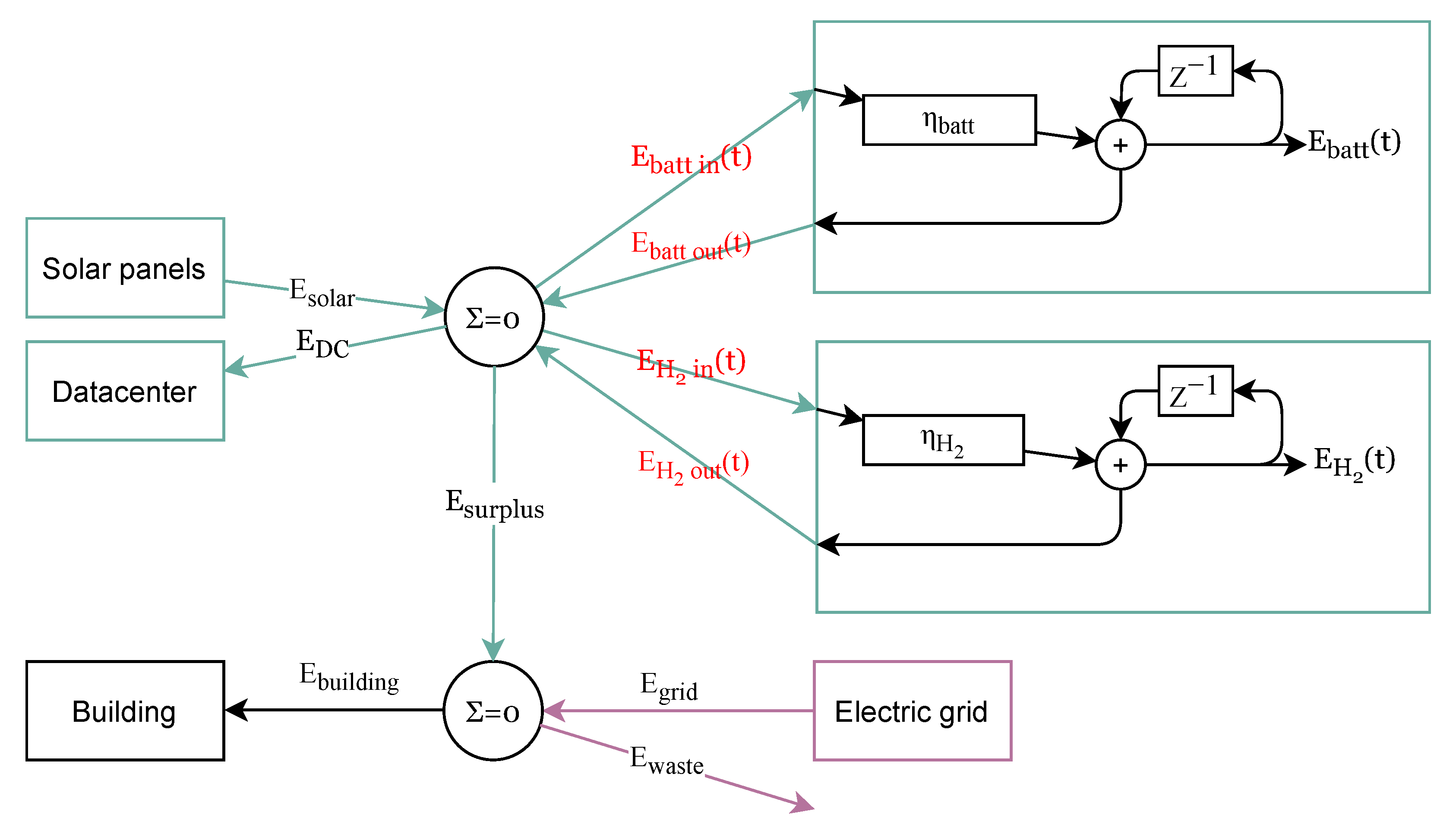
Energy storage is a crucial question for the usage of photovoltaic (PV) energy because of its time-varying behavior. In the ÉcoBioH2 project [1], we consider a building with solar panels providing different usages. The building includes a datacenter that is constrained to be powered by solar energy. It has a low carbon footprint building with lead and hydrogen storage capabilities. Our goal is to monitor this hybrid energy storage system with a goal of low carbon impact.

The building [1] is partially islanded with a datacenter that can only be powered by the energy produced by the building’s solar panels. The proportion of energy produced by the PV in the energy consumed by the building, including the datacenter, defines the self-consumption. The EcoBioH2 project requests the self-consumption to be at least 35%. Demand flexibility, where the load is adjusted to meet production, is not an option in this building so that energy storage will be needed to power the datacenter. Daily variations of the energy production can be mitigated using lead or lithium batteries. However, due to their low capacity density such technologies cannot be used for interseasonal storage. Hydrogen energy storage, on the other hand, is a promising solution to this problem, enabling yearly low-volume, high-capacity, low-carbo-emission energy storage. Unfortunately, it is plagued by its low storage efficiency. Combining hydrogen storage with lead batteries in a hybrid energy storage system enables us to leverage the advantages of both energy storages [2]. Hybrid storage has been shown to perform well in islanded emergency situations [3]. Lead batteries can deliver a big load but not for long. On the other hand, hydrogen storage only supports a small load but has a higher capacity than lead or lithium batteries allowing a longer discharge. The question becomes how to monitor the charge and discharge of each storage and to balance between the short-term battery and the long-term hydrogen storage?

We encounter therefore several short and long-term goals and constraints in opposition summarized in Table 1. Minimizing the carbon impact discourages from using batteries, as batteries emit carbon during their lifecycle. It also encourages using $H_2$ storage when needed, as less carbon is emitted per kW·h than battery storage. The less energy is stored, the less energy is lost in storage efficiency. This results in more energy available to the building. Thus, in the short-term, self-consumption increases. However, the datacenter is not guaranteed to have enough energy available for the long-term. Keeping the datacenter powered by solar energy requires storing as much energy as possible. Nevertheless, some energy is lost during charge and discharge leading to a lower self-consumption. This energy should be stored in the battery first since less energy is lost in efficiency, resulting in higher emissions. Keeping the datacenter powered is a long-term objective as previous decisions impact the current state that constraints our capacity to power the datacenter in the future. Nonetheless, because of their capacities our energy storage systems perform in opposition. Battery storage has a limited capacity. It allows the withstanding of short-term production variations. Hydrogen storage has an enormous capacity. It helps with long-term, interseasonal variations.

Table 1. Contradictory consequences of carbon impact minimization and datacenter powering.

Minimizing Carbon Impact	Keeping the Datacenter Powered
short duration	long duration
high self-consumption	low self-consumption
use only $H_2$	charge batteries first
do not need any capacity	need large hydrogen storage capacity

Managing a long-term storage system means that the control system needs to choose actions (charge or discharge and storage type) depending on their long-term consequences. We consider a duration of several months. We want to minimize the carbon impact while having enough energy for a complete year at least, under the constraints of the datacenter being powered by solar energy. Using convex optimization to solve this problem requires precise forecasting of the energy production and consumption for the whole year. One cannot have months of such forecasts in advance [4,5]. In [6], the authors try to minimize the cost and limit their study to 3 days only. Methods based on genetic algorithms, as [7], require a detailed model of the building usages and energy production which is not realistic in our case since all parts are not known in advance. We also want to allow flexible usages. Therefore, we propose to adopt a solution that can cope with light domain expertise. If the input and output data of the problem are accessible, supervised learning and deep learning can be considered [8]. Having contradicting goals with different horizons, reinforcement learning is an interesting approach [9]. The solution we are looking for should provide a suitable control policy for our hybrid storage system. Most reinforcement learning methods quantize the action space to avoid having interdependent action space bounds [10]. However, such a solution comes with a loss in precision in the action’s selection. It requires more data for learning.

Taking into account theses aspects, we address in the sequel our problem formulation allowing the deployment of non-quantized Deep Reinforcement Learning (DRL) [11] to learn the storage decision policy. DRL learns a long-term evaluation of actions and uses it to train an actor that for each state of the building gives the best action. In our case, the action is the charge or discharge of the lead and hydrogen storages. Learning the policy could even improve controlling the efficiency in the short-term [12]. Existing works focus on non-islanded settings [13] where no state causes a failure. Since our building is partially islanded, this approach would yield to a failure where the islanded portion is not powered anymore. Existing DRL for hybrid energy storage systems focuses on minimizing the energy cost [14]. It does not consider the minimization of carbon emission in a partially islanded building.

In this paper, we formulate the carbon impact minimization of the partially islanded building to learn a hybrid storage policy using DRL. We will reformulate this problem to reduce the action space dimension and therefore improve the DRL performance.

The contributions of this paper are as follows:

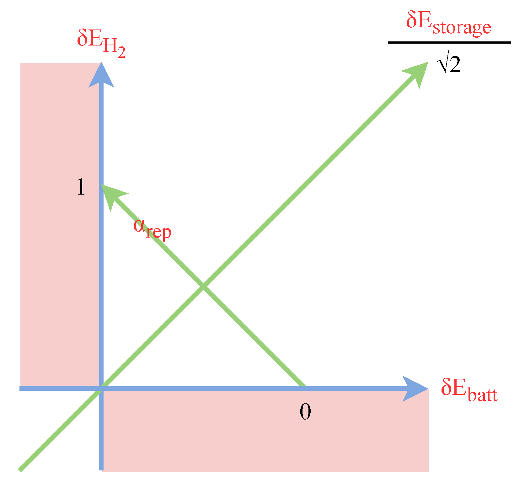
• We redefine the action space so that the action bounds are not interdependent.
• We use this reformulation to reduce the action space to a single dimension.
• From this analysis, we deduce a fixed up to a projection (but not learned) repartition policy between the lead and hydrogen.
• We propose an actor–critic approach to control the partially islanded hybrid energy storage of the building, to be named DDPG${\alpha }_{\mathbf{rep}}$.

Simulations will show the importance of the hydrogen efficiency and carbon impact normalization in the reward, for the learned policy to be effective.

2. Problem Statement

In this section, we describe the model used to simulate our building. This model is sketched in Figure 1 and explained next. Action variables are noted in red.

Figure 1. View of our system. lines in green shows the solar-only part and purple lines shows the grid-only part. actions are displayed in red.

2.1. Storages

We use a simplified model of the energy storage elements as they are sufficient to validate the learning approach for our hybrid storage problem. However, the proposed learning approach can use any batteries model or data since the proposed reformulations and learning do not depend on the batteries model. As long as the action is limited to how much we should charge or discharge, any storage model can be used instead. Since we propose a learning approach, the learned policy could be further improved using real data. Both energy storages (lead battery and $H_2$) use the same equations:

$$E_{H_2}\left(t\right)=E_{H_2}(t-1)+{\eta }_{H_2}{E}_{H_{2}in}\left(t\right)-E_{H_{2}out}\left(t\right)$$

(1)

with $E_{H_2}\left(t\right)$ the state of health of the $H_2$ storage at instant t, ${\eta }_{H_2}$ the global (charging electrolyser and discharging proton-exchange membrane fuel cells) efficiency of $H_2$ storage. $E_{H_{2}in}\left(t\right)$ is the charge energy and $E_{H_{2}out}\left(t\right)$ is the energy discharged at instant t. Equation (1) must satisfy the following constraints:

$$\begin{array}{c}0\le E_{H_2}\left(t\right)\le E_{H_{2}max}\end{array}$$

(2)

$$\begin{array}{c}0\le E_{H_{2}in}\left(t\right)\le E_{H_{2}inmax}\end{array}$$

(3)

$$\begin{array}{c}0\le E_{H_{2}out}\left(t\right)\le E_{H_{2}outmax}\end{array}$$

(4)

with $E_{H_{2}max}$, $E_{H_{2}inmax}$ and $E_{H_{2}outmax}$ the respective upper bounds for $E_{H_2}\left(t\right)$, $E_{H_{2}in}\left(t\right)$ and $E_{H_{2}out}\left(t\right)$. To obtain the lead battery equations replace $H_2$ by $batt$ in Equations (1)–(4). The lead battery efficiency ${\eta }_{batt}$ covers the whole battery efficiency: charge and discharge

2.2. Solar Circuit

The solar circuit connects elements that manage the solar energy only. The production is provided by solar panels $E_{solar}\left(t\right)$. Part of this energy will be stored in short-term (lead battery) or long-term (hydrogen) storage. Part of this energy will be consumed directly by a small datacenter, $E_{DC}\left(t\right)$. The solar circuit is not allowed to handle grid electricity. We define $E_{surplus}\left(t\right)$ as:

$$E_{surplus}\left(t\right)=E_{solar}\left(t\right)-E_{DC}\left(t\right)+E_{battout}\left(t\right)-E_{battin}\left(t\right)+E_{H_{2}out}\left(t\right)-E_{H_{2}in}\left(t\right)$$

(5)

Please note that this equation does not prevent from charging one energy storage by the other. The solar circuit can only give energy to the general circuit, so that:

$$E_{surplus}\left(t\right)\ge 0$$

(6)

This constraint (6) ensures that the datacenter can only be provided in solar energy, as is required by our project [1]. $E_{solar}\left(t\right)$ values are computed using irradiance values from [15] and physical properties of our solar panels.

2.3. General Circuit

The building consumption $E_{building}\left(t\right)$ values come from EcoBio$H_2$ technical office study [16]. They take into account the power consumption of the housing, the restaurant, ...and other usages that are hosted by the building. We define $\delta E_{regul}\left(t\right)$ as the difference between $E_{building}\left(t\right)$ and $E_{surplus}\left(t\right)$:

$$\delta E_{regul}\left(t\right)=E_{building}\left(t\right)-E_{surplus}\left(t\right)$$

(7)

When $\delta E_{regul}\left(t\right)>0$, we define it as the consumption from the electric grid:

$$E_{grid}\left(t\right)=max(0,\delta E_{regul}\left(t\right))$$

(8)

When $\delta E_{regul}\left(t\right)<0$, we define it as the energy discarded since this building is not allowed to give energy back to the grid:

$$E_{waste}\left(t\right)=max(0,-\delta E_{regul}\left(t\right))$$

(9)

In reality, the energy discarded will not be produced. This will be done by temporarily disconnecting the solar panels.

We define $E_{grid}\left(t\right)$ and $E_{waste}\left(t\right)$ in Equations (8) and (9) as they are used in the simulation metrics in Section 5.2. Variables defined previously and in the remaining of this paper are displayed in Table 2, parameters are in Table 3.

Table 2. Nomenclature of variables used.

Symbol	Meaning
$E_{H_2}\left(t\right)$	hydrogen storage state of charge at instant t
$E_{H_2 \mathit{in}}\left(t\right)$	hydrogen storage charge at instant t
$E_{H_2 \mathit{out}}\left(t\right)$	hydrogen storage discharge at instant t
$E_{batt}\left(t\right)$	lead storage state of charge at instant t
$E_{bat\mathit{t\; in}}\left(t\right)$	lead storage charge at instant t
$E_{bat\mathit{t\; out}}\left(t\right)$	lead storage discharge at instant t
$E_{\mathit{solar}}\left(t\right)$	Solar production for the hour
$E_{DC}\left(t\right)$	Datacenter consumption for the hour
$E_{sur plus}\left(t\right)$	Energy going from the solar circuit to the general one
$E_{\mathit{building}}\left(t\right)$	Energy consumed by the building, excluding the datacenter
$E_{grid}\left(t\right)$	Energy coming from the grid
$E_{waste}\left(t\right)$	Energy overproduced for the building
t	time step
at	action vector at instant t
st	state vector at instant t
$f(\mathbf{s},\mathbf{a})$	carbon impact in state $\mathbf{s}$ doing action $\mathbf{a}$
$R(\mathbf{s},\mathbf{a})$	reward in state $\mathbf{s}$ doing action $\mathbf{a}$
$r_t$	reward in state st doing action at
${\delta E}_{batt}\left(t\right)$	lead battery contribution
${\delta E}_{H_2}\left(t\right)$	Hydrogen storage contribution
${\delta E}_{\mathit{storage}}\left(t\right)$	Global energy storages contribution
${\alpha }_{\mathit{rep}}\left(t\right)$	Energy storages contribution repartition
$Q({\mathbf{s}}_t,{\mathbf{a}}_t)$	discounted sum of future reward doing action at in state st
$y_t$	estimation of $Q({\mathbf{s}}_t,{\mathbf{a}}_t)$ used in the critic loss
$\gamma$	discount factor of future rewards
$\pi \left(\mathbf{s}\right)$	policy returning an action $\mathbf{a}$ in state $\mathbf{s}$
${\varphi }_i$	critic parameters at time step i
${\theta }_i$	policy parameters at time step i
$J\left({\varphi }_i\right)$	critic loss
${\varphi }_{oldi}$	critic parameters at time step i
${\theta }_{oldi}$	policy parameters at time step i
$\mu$	step-size for critic learning
$\lambda$	step-size for actor learning
$\tau$	stabilization networks update proportion
N	duration: average length of a policy
s	self-consumption ratio (62)

Table 3. Parameters values used during simulations.

Quantity	Value	Unit
${\eta }_{solaropacity}$	0.6
${\eta }_{solar}$	0.21
$S_{panels}$	1000	m${}^2$
$C_{solar}$	55	gCO${}_2$eq/kW·h
$E_{solarMax}$	185	kW·h
${\eta }_{batt}$	0.81
$C_{battIn}$	68.66	gCO${}_2$eq/kW·h
$C_{battOut}$	86	gCO${}_2$eq/kW·h
$E_{battMax}$	650 / 2	kW·h
$E_{battInMax}$	$E_{battMax}$	kW·h
$E_{battOutMax}$	$E_{battMax}$	kW·h
${\eta }_{H_2}$	0.35
$C_{H_{2}In}$	1.75	gCO${}_2$2eq/kW·h
$C_{H_{2}Out}$	5	gCO${}_2$2eq/kW·h
$E_{H_{2}Max}$	1000	kW·h
$E_{H_{2}InMax}$	$2\times 10$	kW·h
$E_{H_{2}OutMax}$	$2\times 5$	kW·h
$C_{grid}$	53	gCO${}_2$eq/kW·h
$E_{DCmax}$	10	kW·h
$E_{buildingMax}$	100	kW·h

2.4. Long-Term Carbon Impact Minimization Problem

We gather the building consumption, the solar panels production at instant t and the previous stored energy state at $t-1$ variables in a so-called state defined as:

$${\mathbf{s}}_t=[E_{building}\left(t\right),E_{solar}\left(t\right),E_{batt}(t-1),E_{H_2}(t-1)]$$

(10)

We define the action variables in

$${\mathbf{a}}_t=[E_{battin}\left(t\right),E_{battout}\left(t\right),E_{H_{2}in}\left(t\right),E_{H_{2}out}\left(t\right)]$$

(11)

to control the energy storage at the current hour t. We define in Equation (12) the instantaneous carbon impact at state ${\mathbf{s}}_t$ when performing action ${\mathbf{a}}_t$ as $f({\mathbf{s}}_t,{\mathbf{a}}_t)$:

$$\begin{array}{cc}\hfill f({\mathbf{s}}_t,{\mathbf{a}}_t)& =C_{solar}{E}_{solar}\left(t\right)+C_{battout}{E}_{battout}\left(t\right)+C_{battin}{E}_{battin}\left(t\right)+C_{H_{2}out}{E}_{H_{2}out}\left(t\right)+C_{H_{2}in}{E}_{H_{2}in}\left(t\right)\hfill \\ \hfill & +C_{grid}\left(t\right)max(0,E_{building}\left(t\right)+E_{DC}\left(t\right)-E_{solar}\left(t\right)-E_{battout}\left(t\right)+E_{battin}\left(t\right)-E_{H_{2}out}\left(t\right)+E_{H_{2}in}\left(t\right))\hfill \end{array}$$

(12)

with $C_{solar}$ the carbon intensity per kW·h from the complete lifecycle of PV usage. $C_{battin}$, $C_{battout}$, $C_{H_{2}in}$, $C_{H_{2}out}$ are the carbon intensity from the complete lifecycle per kW·h of respectively lead battery charge, discharge, hydrogen storage charge and discharge. $C_{grid}\left(t\right)$ quantifies the carbon emissions per kW·h associated with energy from the grid. Their values for simulations are provided in Table 3. Our goal is to minimize the long-term carbon impact taking into account the carbon emissions at the current and future states ${\mathbf{s}}_t,\cdots ,{\mathbf{s}}_{t+H}$ as induced by the current and future actions ${\mathbf{a}}_t,\cdots ,{\mathbf{a}}_{t+H}$:

$${\mathbf{a}}_t=arg\underset{{\mathbf{a}}_t}{min}\sum _{h=0}^{H}f({\mathbf{s}}_{t+h},{\mathbf{a}}_{t+h})$$

(13)

under the constraints (2), (3), (4) and (6). We call this initial formulation $\mathbf{TwoBatts}$.

The challenge comes from our ignorance of the actions that will be taken in the future ${\mathbf{a}}_{t+1},\cdots ,{\mathbf{a}}_{t+H}$. Yet, we need to account for their impact. DRL approaches are meant for such kind of challenges.

3. Problem Reformulations

In this section, we reformulate our problem (13) to simplify its resolution. We consider in particular the reduction of the action space to reduce the complexity and improve the convergence of learning.

3.1. Battery Charge or Discharge

The current formulation of our problem, TwoBatts, allows the policy to charge and discharge a battery simultaneously. We note that the cost function to be minimized (12) is increasing with the different components of ${\mathbf{a}}_t$. This leads to multiple actions that, in the same state ${\mathbf{s}}_t$, yield to the same ${\mathbf{s}}_{t+1}$ while having different costs. To avoid having to deal with such cases, we impose that the energy storage systems can only be charged or discharged at a given instant t:

$$E_{battin}\left(t\right)\times E_{battout}\left(t\right)=0$$

(14)

Therefore, we express the charge and discharge of each battery in a single dimension:

$$\begin{array}{c}\delta E_{batt}\left(t\right):=E_{battout}\left(t\right)-E_{battin}\left(t\right)\end{array}$$

(15)

$$\begin{array}{c}\delta E_{H_2}\left(t\right):=E_{H_{2}out}\left(t\right)-E_{H_{2}in}\left(t\right)\end{array}$$

(16)

We propose to use these new variables as the action space:

$${\mathbf{a}}_t=[\delta E_{batt}\left(t\right),\delta E_{H_2}\left(t\right)]$$

(17)

To obtain the new model equations, we replace the following variables in Equations (1)–(12):

$$\begin{array}{cc}\hfill E_{battout}\left(t\right)& :=max(\delta E_{batt}\left(t\right),0)\hfill \end{array}$$

(18)

$$\begin{array}{cc}\hfill E_{battin}\left(t\right)& :=max(-\delta E_{batt}\left(t\right),0)\hfill \end{array}$$

(19)

$$\begin{array}{cc}\hfill E_{H_{2}out}\left(t\right)& :=max(\delta E_{H_2}\left(t\right),0)\hfill \end{array}$$

(20)

$$\begin{array}{cc}\hfill E_{H_{2}in}\left(t\right)& :=max(-\delta E_{H_2}\left(t\right),0)\hfill \end{array}$$

(21)

Thus, we obtain the formulation 2Dbatt of (13) with

$$\begin{array}{cc}\hfill f({\mathbf{s}}_t,{\mathbf{a}}_t)& =C_{solar}{E}_{solar}\left(t\right)\hfill \\ \hfill & +C_{battout}max(\delta E_{batt}\left(t\right),0)+C_{battin}max(-\delta E_{batt}\left(t\right),0)\hfill \\ \hfill & +C_{H_{2}out}max(\delta E_{H_2}\left(t\right),0)+C_{H_{2}in}max(-\delta E_{H_2}\left(t\right),0)\hfill \\ \hfill & +C_{grid}\left(t\right)max(E_{building}\left(t\right)+E_{DC}\left(t\right)-E_{solar}\left(t\right)-\delta E_{batt}\left(t\right)-\delta E_{H_2}\left(t\right),0)\hfill \end{array}$$

(22)

Next, we revisit the constraints with this new action space. When we only charge ($\delta E_{H_2}\left(t\right)=-E_{H_{2}in}\left(t\right)$), straightforward calculations result in (2) being equivalent to

$$\begin{array}{cc}\hfill -\frac{E_{H_{2}max}-E_{H_2}(t-1)}{{\eta }_{H_2}}& \le \delta E_{H_2}\left(t\right)\hfill \end{array}$$

(23)

and (3) turns into:

$$\begin{array}{c}-E_{H_{2}inmax}\le \delta E_{H_2}\left(t\right)\end{array}$$

(24)

When we only discharge ($\delta E_{H_2}\left(t\right)=E_{H_{2}out}\left(t\right)$) (2) becomes:

$$\begin{array}{cc}\hfill \delta E_{H_2}\left(t\right)& \le E_{H_2}(t-1)\hfill \end{array}$$

(25)

Accordingly, (4) is equivalent to:

$$\begin{array}{c}\delta E_{H_2}\left(t\right)\le E_{H_{2}outmax}\end{array}$$

(26)

The battery is constrained by variations of (23)–(26). Both storages are constrained by Equation (6) that turns into:

$$0\le E_{solar}\left(t\right)-E_{DC}\left(t\right)+\delta E_{batt}\left(t\right)+\delta E_{H_2}\left(t\right)$$

(27)

The 2Dbatt formulation is the minimization of (13) over (17) constrained by Equations (23)–(26), their battery variant and (27).

3.2. Batteries Storage Repartition

In the 2Dbatt formulation, one storage can discharge when the other is charging which results in a loss of energy. Moreover, the actions bound (27) depends not only on the state but also on the action itself. The bounds are therefore interdependent. If we select an action outside the action bounds, there is a need to project it inside the bounds which is non-trivial because of this interdependence.

To alleviate this problem, we propose to rotate the action space frame. We merge the two action dimensions into the energy storage systems contribution and the contribution repartition defined as:

$$\begin{array}{c}\delta E_{storage}\left(t\right):=\delta E_{batt}\left(t\right)+\delta E_{H_2}\left(t\right)\end{array}$$

(28)

$$\begin{array}{c}{\alpha }_{rep}\left(t\right):=\frac{\delta E_{H_2}\left(t\right)}{\delta E_{storage}\left(t\right)}\end{array}$$

(29)

so that the action becomes ${\mathbf{a}}_t=[\delta E_{storage}\left(t\right),{\alpha }_{rep}\left(t\right)]$. ${\alpha }_{rep}\left(t\right)$ is the proportion of hydrogen in the storing. It is equal to 0 when the sole battery storage is used and to 1 when only the hydrogen storage is used. ${\alpha }_{rep}\left(t\right)$ is bounded between 0 and 1 by definition, so that one energy storage cannot charge the other. Furthermore, we only convert from Repartition to 2Dbatts and not the other way around. This is illustrated in Figure 2. To insert the new variables in the 2Dbatt formulation, we use the following equations:

$$\begin{array}{c}\delta E_{batt}\left(t\right)=(1-{\alpha }_{rep}\left(t\right))\times \delta E_{storage}\left(t\right)\end{array}$$

(30)

$$\begin{array}{c}\delta E_{H_2}\left(t\right)={\alpha }_{rep}\left(t\right)\times \delta E_{storage}\left(t\right)\end{array}$$

(31)

Figure 2. Repartition formulation (green), $\delta E_{storage}\left(t\right)$ and ${\alpha }_{rep}\left(t\right)$, in the 2Dbatt (blue) action space. Actions where one storage is charged and the other discharged are highlighted in red.

We transform Equations (23)–(26) using (31):

$$\begin{array}{c}-\frac{E_{H_{2}max}-E_{H_2}(t-1)}{{\eta }_{H_2}}\le {\alpha }_{rep}\left(t\right)\times \delta E_{storage}\left(t\right)\end{array}$$

(32)

$$\begin{array}{c}-E_{H_{2}inmax}\le {\alpha }_{rep}\left(t\right)\times \delta E_{storage}\left(t\right)\end{array}$$

(33)

$$\begin{array}{c}{\alpha }_{rep}\left(t\right)\times \delta E_{storage}\left(t\right)\le E_{H_2}(t-1)\end{array}$$

(34)

$$\begin{array}{c}{\alpha }_{rep}\left(t\right)\times \delta E_{storage}\left(t\right)\le E_{H_{2}outmax}\end{array}$$

(35)

We obtain the battery variant of those equations using (31):

$$\begin{array}{c}-\frac{E_{battmax}-E_{batt}(t-1)}{{\eta }_{batt}}\le (1-{\alpha }_{rep}\left(t\right))\times \delta E_{storage}\left(t\right)\end{array}$$

(36)

$$\begin{array}{c}-E_{battinmax}\le (1-{\alpha }_{rep}\left(t\right))\times \delta E_{storage}\left(t\right)\end{array}$$

(37)

$$\begin{array}{c}(1-{\alpha }_{rep}\left(t\right))\times \delta E_{storage}\left(t\right)\le E_{batt}(t-1)\end{array}$$

(38)

$$\begin{array}{c}(1-{\alpha }_{rep}\left(t\right))\times \delta E_{storage}\left(t\right)\le E_{battoutmax}\end{array}$$

(39)

Moreover, using (28), (27) becomes:

$$E_{DC}\left(t\right)-E_{solar}\left(t\right)\le \delta E_{storage}\left(t\right)$$

(40)

Equation (40) depends only on one variable, $\delta E_{storage}\left(t\right)$. Using this variable change, we have removed the interdependency of the constraint in (27).

Next, we propose bounds on $\delta E_{storage}\left(t\right)$ and ${\alpha }_{rep}\left(t\right)$ that will be critical in the sequel.

Proposition 1.

$\delta E_{storage}\left(t\right)$ is constrained by $\delta E_{storagemin}\left(t\right)\le \delta E_{storage}\left(t\right)\le \delta E_{storagemax}\left(t\right)$ and their values are defined by:

$$\begin{array}{cc}\hfill \delta E_{storagemin}\left(t\right)=max(& E_{DC}\left(t\right)-E_{solar}\left(t\right),\hfill \\ \hfill & -E_{battinmax}-E_{H_{2}inmax},\hfill \\ \hfill & -\frac{E_{battmax}-E_{batt}(t-1)}{{\eta }_{battin}}-\frac{E_{H_{2}max}-E_{H_2}(t-1)}{{\eta }_{H_{2}in}},\hfill \\ \hfill & -E_{battinmax}-\frac{E_{H_{2}max}-E_{H_2}(t-1)}{{\eta }_{H_{2}in}},\hfill \\ \hfill & -\frac{E_{battmax}-E_{batt}(t-1)}{{\eta }_{battin}}-E_{H_{2}inmax})\hfill \end{array}$$

(41)

$$\begin{array}{cc}\hfill \delta E_{storagemax}\left(t\right)=min(& E_{batt}(t-1)+E_{H_2}(t-1),\hfill \\ \hfill & E_{battoutmax}+E_{H_2}(t-1),\hfill \\ \hfill & E_{batt}(t-1)+E_{H_{2}outmax},\hfill \\ \hfill & E_{battoutmax}+E_{H_{2}outmax})\hfill \end{array}$$

(42)

Proof of Proposition 1 is in Appendix A.

Proposition 2.

${\alpha }_{rep}\left(t\right)$ is constrained by ${\alpha }_{repmin}\left(t\right)\le {\alpha }_{rep}\left(t\right)\le {\alpha }_{repmax}\left(t\right)$ with values are defined by:

$${\alpha }_{repmin}\left(t\right)=\left\{\begin{array}{c}\begin{array}{cc}\hfill max(1& +\frac{E_{battinmax}}{\delta E_{storage}\left(t\right)},\hfill \\ \hfill 1& +\frac{E_{battmax}-E_{batt}(t-1)}{{\eta }_{batt}\times \delta E_{storage}\left(t\right)})\hfill \end{array}\mathit{if}\delta E_{storage}\left(t\right)<0\hfill \\ \begin{array}{cc}\hfill max(1& -\frac{E_{batt}\left(t\right)-1}{\delta E_{storage}\left(t\right)},\hfill \\ \hfill 1& -\frac{E_{battoutmax}}{\delta E_{storage}\left(t\right)})\hfill \end{array}\mathit{if}\delta E_{storage}\left(t\right)>0\hfill \end{array}\right.$$

(43)

$${\alpha }_{repmax}\left(t\right)=\left\{\begin{array}{c}\begin{array}{cc}\hfill min(& -\frac{E_{H_{2}inmax}}{\delta E_{storage}\left(t\right)},\hfill \\ \hfill & -\frac{E_{H_{2}max}-E_{H_2}(t-1)}{{\eta }_{H_2}\times \delta E_{storage}\left(t\right)})\hfill \end{array}\mathit{if}\delta E_{storage}\left(t\right)<0\hfill \\ \begin{array}{cc}\hfill min(& \frac{E_{H_2}t-1}{\delta E_{storage}\left(t\right)},\hfill \\ \hfill & \frac{E_{H_{2}outmax}}{\delta E_{storage}\left(t\right)})\hfill \end{array}\mathit{if}\delta E_{storage}\left(t\right)>0\hfill \end{array}\right.$$

(44)

Proof of Proposition 2 is in Appendix B. Please note that when $\delta E_{storage}\left(t\right)=0$, ${\alpha }_{rep}\left(t\right)$ does not matter. We will set it to ${\alpha }_{rep}\left(t\right)=0.5$ as a convention.

The interest of bounds (43) and (44) is that they depend on $\delta E_{storage}\left(t\right)$ only, whereas the bounds on $\delta E_{storage}\left(t\right)$ do not depend on ${\alpha }_{rep}\left(t\right)$. Thus, given $\delta E_{storage}\left(t\right)$, we only need to decide the contribution of the distribution ${\alpha }_{rep}\left(t\right)$. The interdependence has been completely removed.

Moreover, we use (30) and (31) to obtain the expression of the modified carbon impact function (12):

$$\begin{array}{cc}\hfill f({\mathbf{s}}_t,{\mathbf{a}}_t)& =C_{solar}{E}_{solar}\left(t\right)\hfill \\ \hfill & +C_{grid}\left(t\right)max(0,E_{building}\left(t\right)+E_{DC}\left(t\right)-E_{solar}\left(t\right)-\delta E_{storage}\left(t\right))\hfill \\ \hfill & +\left\{\begin{array}{c}\begin{array}{cc}\hfill & C_{battout}\times (1-{\alpha }_{rep}\left(t\right))\times \delta E_{storage}\left(t\right)\hfill \\ \hfill +& C_{H_{2}out}\times {\alpha }_{rep}\left(t\right)\times \delta E_{storage}\left(t\right)\hfill \end{array}\hfill \\ \hfill \mathrm{if}\delta E_{storage}\left(t\right)>0\\ \\ \begin{array}{cc}\hfill -& C_{battin}\times (1-{\alpha }_{rep}\left(t\right))\times \delta E_{storage}\left(t\right)\hfill \\ \hfill -& C_{H_{2}in}\times {\alpha }_{rep}\left(t\right)\times \delta E_{storage}\left(t\right)\hfill \end{array}\hfill \\ \hfill \mathrm{if}\delta E_{storage}\left(t\right)<0\end{array}\right.\hfill \end{array}$$

(45)

The problem (13) with action ${\mathbf{a}}_t=[\delta E_{storage}\left(t\right),{\alpha }_{rep}\left(t\right)]$, the carbon impact (45) and under the constraints (41)–(44) is called the Repartition formulation.

3.3. Repartition Parameter Only

We have noticed that $\delta E_{storage}\left(t\right)$ can be seen as a single global storage. To provide energy for as long a duration as possible, i.e., to respect (40), we want to charge as much as possible and discharge only when needed. We call this the frugal policy. It corresponds to $\delta E_{storage}\left(t\right)$ being equal to its lower bound:

$$\delta E_{storage}\left(t\right)=\delta E_{storagemin}\left(t\right)$$

(46)

To reduce even more the action space dimensionality, we propose to use the frugal policy and to focus on learning only ${\alpha }_{rep}\left(t\right)$ the repartition between the lead and hydrogen energy storage systems contribution.

Using this remark, we propose the ${\alpha }_{\mathbf{rep}}$ reformulation with the goal (13), in order to find the single action ${\mathbf{a}}_t={\alpha }_{rep}\left(t\right)$, given the state ${\mathbf{s}}_t$, using the carbon impact (45) and under constraints (43) and (44) with $\delta E_{storage}\left(t\right)$ derived in (46). Unless specified, this is the formulation we use in the sequel of this paper.

3.4. Fixed Repartition Policy

In Section 4, we will propose a learning algorithm for the different formulations. To show the interest of learning, we want to compare the learned policies to a frugal policy (46) where ${\alpha }_{rep}\left(t\right)$ is preselected and fixed to a value v. At each instant, we will only verify that $v\in [{\alpha }_{min}\left(t\right),{\alpha }_{max}\left(t\right)]$ and project it into this interval otherwise. We call ${\alpha }_{\mathbf{rep}}=\mathbf{v}$ the policy where ${\alpha }_{rep}$ is preset to value v. So that:

$${\alpha }_{rep}\left(t\right)={\mathrm{projection}}_{[{\alpha }_{repmin}\left(t\right),{\alpha }_{repmax}\left(t\right)]}\left(v\right)$$

(47)

In Section 1, we explained that the battery is intended for short-term storage and that the $H_2$ storage is intended for long-term. Our intuition therefore suggests charging or discharging the lead battery first. This corresponds to a preset value of ${\alpha }_{\mathbf{rep}}=\mathbf{0}$, so that ${\alpha }_{rep}\left(t\right)={\alpha }_{repmin}\left(t\right)$.

One should wonder, what is the best preselected ${\alpha }_{rep}$? To find it, we simulated 100 different values of ${\alpha }_{rep}$ between 0 and 1. For each value v, we run a simulation for each day starting at midnight on a looping year 2006. A detailed description of this data is available in Section 5.1. We use the parameters in Table 3 and PV production computed using irradiance data [17,18] in (48):

$$E_{solar}\left(t\right)=P_{solar}\left(t\right){\eta }_{solar}{\eta }_{solaropacity}{S}_{panels}$$

(48)

If the simulation does not last the whole year, we reject it (hatched area in Figure 3). Otherwise, we compute the hourly carbon impact:

$$\sum _{t=0}^T\frac{f(s_t,a_t)}{T}$$

(49)

with T the number of hours in 2006. This hourly impact is averaged over 365 different runs, each starting at midnight, one for each day of 2006. Figure 3 shows the carbon impact versus ${\alpha }_{rep}$. The ${\alpha }_{rep}$ value that minimizes the average hourly impact while lasting the whole year is therefore ${\alpha }_{\mathbf{rep}}=\mathbf{0.2}$. It will be used for comparison.

Figure 3. Mean impact versus ${\alpha }_{rep}$ preset. Hatched area corresponds to rejected ${\alpha }_{rep}$ values where the policy does not last the whole year.

4. Learning the Policy with DDPG

In the reformulation ${\alpha }_{\mathbf{rep}}$ reformulation, we want to select ${\mathbf{a}}_t$ given the state ${\mathbf{s}}_t$. The function that provides ${\mathbf{a}}_t$ given ${\mathbf{s}}_t$ is referred to as the policy. We want to learn the policy using DRL with an actor–critic policy-based approach: the Deep Deterministic Policy Gradient (DDPG) [19]. Experts may want to skip Section 4.2 and Section 4.3.

4.1. Actor–Critic Approach

We call $env$ for the environment, the set of equations: (1) and its battery variant that allows the obtaining of ${\mathbf{s}}_{t+1}$ from ${\mathbf{a}}_t$ and ${\mathbf{s}}_t$, ${\mathbf{s}}_{t+1}=env.step({\mathbf{s}}_t,{\mathbf{a}}_t)$. Its corresponding reward, the short-term evaluation function, is defined as a function of ${\mathbf{s}}_t$ and ${\mathbf{a}}_t$, $r_t=R({\mathbf{s}}_t,{\mathbf{a}}_t)$. 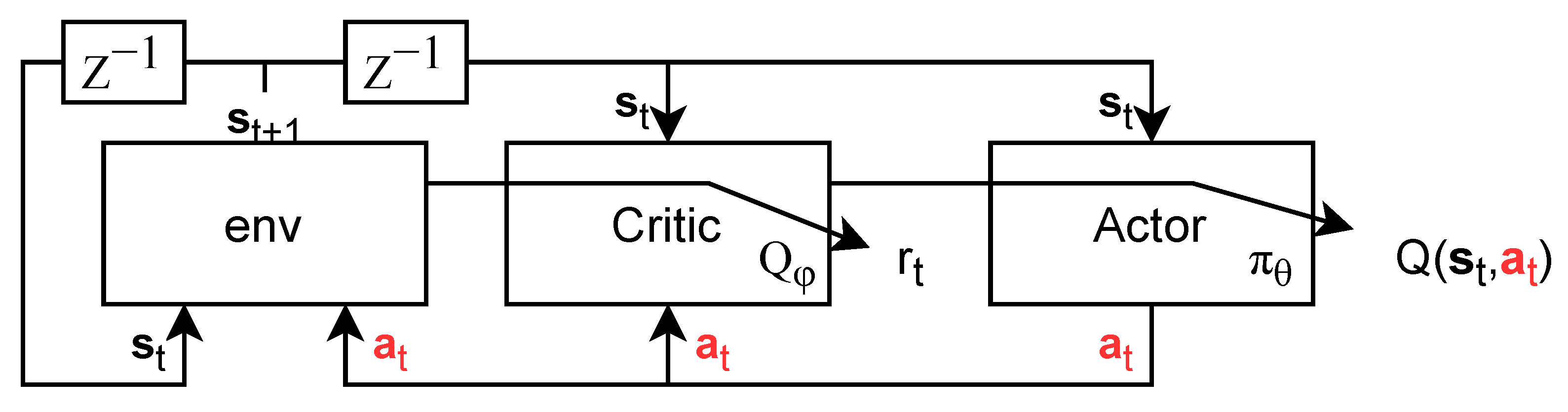We use [19], an actor–critic approach, where the estimated best policy for a given environment ${\mathbf{s}}_{t+1}=env.step({\mathbf{s}}_t,{\mathbf{a}}_t)$ is learned through a critic as in Figure 4. The critic transforms this short-term evaluation into a long-term evaluation, the Q-values $Q({\mathbf{s}}_t,{\mathbf{a}}_t)$, through learning. It will be detailed in Section 4.2. The actor ${\pi }_{\theta }:{\mathbf{s}}_t\to {\mathbf{a}}_t$ is the function that selects the best possible action ${\mathbf{a}}_t$ possible. It uses the critic as to know what is the best action in a given state (as detailed in Section 4.3).

Figure 4. Overview of the actor–critic approach. Curved arrows indicate learning. Time passing with $t=t+1$ is displayed $Z^{-1}$.

In Section 2.4, we set our objective to minimize the long-term carbon impact (13). However, in reinforcement learning we try to maximize a score, defined as the sum of all rewards:

$$\sum _{t_0}^T{r}_t$$

(50)

To remove this difference, we maximize the negative carbon impact $\sum -f({\mathbf{s}}_t,{\mathbf{a}}_t)$. However, the more negative terms you add, the lower the sum is. This leads to a policy trying to stop the simulation as fast as possible, in contradiction to our goal to always provide the datacenter in energy. To counter this, we propose, inspired by [20], to add a living incentive of 1 at each instant. Therefore, we propose to define the reward as:

$$r_t=R({\mathbf{s}}_t,{\mathbf{a}}_t)=1-\frac{f({\mathbf{s}}_t,{\mathbf{a}}_t)}{{max}_{\mathbf{a}}f({\mathbf{s}}_t,\mathbf{a})}$$

(51)

The reward accounting for the carbon impact is now normalized between 0 and 1 so that the reward is always positive. Still in this reward the normalization depends on the state ${\mathbf{s}}_t$. When the normalization depends on the state, two identical actions can have different rewards associated with them. Therefore, the reward is not proportional to the carbon impact (45) making the reward harder to interpret. To alleviate this problem, we propose to use the global maximum instead of the worst case for the current state:

$$r_t=R({\mathbf{s}}_t,{\mathbf{a}}_t)=1-\frac{f({\mathbf{s}}_t,{\mathbf{a}}_t)}{{max}_{\mathbf{s},\mathbf{a}}f(\mathbf{s},\mathbf{a})}$$

(52)

By convention $r_t$ is set to zero after the simulation ends.

The actor and critic are parameterized using artificial neural networks, respectively denoted $\theta$ and $\varphi$. They will be learned alternatively and iteratively. Two stabilization networks are also used for the critic supervision with weights ${\theta }_{old}$ and ${\varphi }_{old}$.

4.2. Critic Learning

Now that we have defined a reward, we can use the critic to transform it into a long-term metric. As time goes, we have less and less trust in the future. Therefore, we discount the future rewards using a discount factor $0<\gamma <1$. We define the critic $Q:{\mathbf{s}}_t,{\mathbf{a}}_t\to {\sum }_{k=0}^{+\infty }{\gamma }^k{r}_{t+k}$. It estimates the weighted long-term returns of taking an action ${\mathbf{a}}_t$ in a given state ${\mathbf{s}}_t$. This weighted version of (50) also allows the binding of the infinite sum to learn it. Q can be expressed recursively:

$$\begin{array}{cc}\hfill Q({\mathbf{s}}_t,{\mathbf{a}}_t)& =\sum _{k=0}^{+\infty }{\gamma }^k{r}_{t+k}\hfill \\ \hfill & =r_t+\gamma \sum _{k=0}^{+\infty }{\gamma }^k{r}_{t+1+k}\hfill \\ \hfill Q({\mathbf{s}}_t,{\mathbf{a}}_t)& =r_t+\gamma Q({\mathbf{s}}_{t+1},{\mathbf{a}}_{t+1})\hfill \end{array}$$

(53)

We learn the Q-function using an artificial neural network of weights $\varphi$. At the $i\mathrm{th}$ iteration of our learning algorithm and for a given value of ${\varphi }_{oldi}$ and ${\theta }_{oldi}$, we define a reference value $y_t$ from the recursive expression (53). Since we do not know ${\mathbf{a}}_{t+1}$, we need to select the best action possible at $t+1$. The best estimator of this action is provided by the policy ${\pi }_{{\theta }_{oldi}}$, so that we define the reference as:

$$y_t=r_t+\gamma Q_{{\varphi }_{oldi}}({\mathbf{s}}_{t+1},{\pi }_{{\theta }_{oldi}}\left({\mathbf{s}}_{t+1}\right))$$

(54)

where ${\mathbf{a}}_{t+1}$ has been estimated by ${\pi }_{{\theta }_{oldi}}\left({\mathbf{s}}_{t+1}\right)$.

The squared difference between the estimated value $Q_{\varphi }({\mathbf{s}}_t,{\mathbf{a}}_t)$, and the reference value $y_t$ [21] is defined as:

$$J\left({\varphi }_i\right)=\sum _{({\mathbf{s}}_t,{\mathbf{a}}_t,r_t,{\mathbf{s}}_{t+1})\in \mathcal{D}}{\left(Q_{{\varphi }_i}({\mathbf{s}}_t,{\mathbf{a}}_t)-y_t\right)}^2$$

(55)

To update ${\varphi }_i$, we minimize $J\left({\varphi }_i\right)$ in (55) using a simple gradient descent:

$${\varphi }_{i+1}={\varphi }_i-\mu \nabla J\left({\varphi }_i\right)$$

(56)

where $\nabla J\left({\varphi }_i\right)$ is the gradient of $J\left(\varphi \right)$ in (55) with respect to $\varphi$ taken at the value ${\varphi }_i$. $\mu$ is a small positive step-size. To stabilize the learning [19] suggests updating the reference network ${\varphi }_{old}$ slower, so that:

$${\varphi }_{oldi+1}=\tau {\varphi }_i+(1-\tau ){\varphi }_{oldi}\mathrm{with}0<\tau \ll 1$$

(57)

${\varphi }_{old0}={\varphi }_0$ at weight initialization.

4.3. Actor Learning

Since we alternate the updates of the critic and of the actor, we address next the learning of the actor. To learn what is the best action to select, we need a loss function that grades different actions ${\mathbf{a}}_t$. Using the reward function (52), as a loss function, the policy would select the best short-term, instantaneous, action. Since the critic $Q({\mathbf{s}}_t,{\mathbf{a}}_t)$ depends on the action ${\mathbf{a}}_t$, we replace ${\mathbf{a}}_t$ by ${\pi }_{\theta }\left({\mathbf{s}}_t\right)$. At iteration i, to update the actor network ${\theta }_i$, we use the gradient ascent of the average $Q_{{\varphi }_i}(\mathbf{s}t,{\pi }_{\theta }\left(\mathbf{s}t\right))$ taken at $\theta ={\theta }_i$. This can be expressed as:

$${\theta }_{i+1}={\theta }_i+\lambda {\nabla \sum }_{({\mathbf{s}}_t,{\mathbf{a}}_t,r_t,{\mathbf{s}}_{t+1})\in \mathcal{D}}{Q}_{{\varphi }_i}\left({\mathbf{s}}_t,{\pi }_{{\theta }_i}\left({\mathbf{s}}_t\right)\right)$$

(58)

where $\lambda$ is a small positive step-size.

To learn the critic a stabilized actor is used. Like the stabilized critic, ${\pi }_{{\theta }_{old}}$ is updated by:

$${\theta }_{oldi+1}=\tau {\theta }_i+(1-\tau ){\theta }_{oldi}\mathrm{with}0<\tau \ll 1$$

(59)

with ${\theta }_{old0}={\theta }_0$ at the beginning.

During learning, an Ornstein–Uhlenbeck noise [22], n, is added to the policy decision to make sure we explore the action space:

$${\mathbf{a}}_t={\pi }_{\theta i}\left({\mathbf{s}}_t\right)+n$$

(60)

4.4. Proposition: DDPG ${\alpha }_{\mathbf{rep}}$ Algorithm to Learn the Policy

From the previous section, we propose the DDPG${\alpha }_{\mathbf{rep}}$ Algorithm 1. This algorithm alternates the learning of the networks of the actor and of the critic. We select randomly the initial instant t to avoid learning time patterns. We start each run with full energy storage.

Once learned, we use the last weights ${\theta }_i$ of the neural network parameterizing the actor to select the action using ${\pi }_{{\theta }_i}:{\mathbf{s}}_t\to {\mathbf{a}}_t$ directly.

To learn well an artificial neural network needs the different samples of learning data to be uncorrelated. In reinforcement learning two consecutive states tends to be close, i.e., correlated. To overcome this problem, we store all experiences $({\mathbf{s}}_t,{\mathbf{a}}_t,r_t,{\mathbf{s}}_{t+1})$ in a memory and use a tiny random subset as the learning batch [23]. The random selection of a batch from the memory is called $sample$.

Algorithm 1: DDPG${\alpha }_{\mathbf{rep}}$

5. Simulation

We have just proposed DDPG${\alpha }_{\mathbf{rep}}$ to learn how to choose ${\alpha }_{rep}\left(t\right)$ with respect to the environment. In this section, we display the simulations settings and results.

5.1. Simulation Settings

Production data are computed using (48) from real irradiance data [17,18] measured at the building location in Avignon, France. The building has $S_{panels}=1000{\mathrm{m}}^2$ of solar panels with ${\eta }_{solaropacity}=60\%$ opacity and an efficiency of ${\eta }_{solar}=21\%$. Those solar panels can produce a maximum of $E_{solarMax}=185$ kW·h per hour.

Consumption data comes from projections of the engineering office [16]. It consists of powering housing units with an electricity demand fluctuating daily between 30 kW·h (1 a.m. to 6 a.m.) and 90 kW·h. The weekly variations of the consumption varies with a factor between 1 and 1.4 during awake hours between workdays and the weekend. There is little interseasonal variation, standard deviation of 0.6 kW·h (0.01% of yearly mean) between seasons, as heating uses wood pellets. In those simulations, the datacenter is consuming a fixed amount of $E_{DCmax}=10$ kW·h. The datacenter consumption adds up to 87.6 MW·h per year, around 17% of the 496 MW·h that the entire building consumes in a year. To power this datacenter, our building’s solar panels produce an average of 53.8 kW·h/h during the $12.7$ sunny hours on average day counts, for a yearly total of 249 MW·h/year. This covers a maximum of 2.8 times the consumption of our datacenter, but lowers to 99% if all energy goes through the hydrogen storage. The same solar production covers at most 50% of the building yearly consumption. When accounting for hydrogen efficiency, the solar production covers at most 17% of the building consumption.

We only use half of the lead battery capacity to preserve the battery health longer $E_{battMax}=650/2=325$ kW·h. The lead battery carbon intensity is split between the charge and discharge $C_{battOut}=172/2=86{\mathrm{gCO}}_2\mathrm{eq}/\mathrm{kW}$·h. Since the charge quantity comes before the efficiency, its carbon intensity must account for efficiency: $C_{battIn}=C_{battOut}{\eta }_{batt}=86\times 0.81=68.66{\mathrm{gCO}}_2\mathrm{eq}/\mathrm{kW}$·h. The carbon intensity of the electrolysers, accounting for the efficiency, is used for $C_{H_{2}in}=5\times {\eta }_{H_2}=1.75{\mathrm{gCO}}_2\mathrm{eq}/\mathrm{kW}$·h. The carbon intensity of the fuel cells corresponds to $C_{H_{2}out}=5{\mathrm{gCO}}_2\mathrm{eq}/\mathrm{kW}$·h. ${\eta }_{H_2}$ account for both the electrolysers and fuel cells efficiency. $C_{grid}=53{\mathrm{gCO}}_2\mathrm{eq}/\mathrm{kW}$·h uses the average French grid carbon intensity. All those values are reported in Table 3.

The simulations use an hourly simulation step t.

We train on the production data from year 2005, validate and select hyperparameters, using best score (50) values, on the year 2006 and test finally on year 2007. Each year lasts 8760 h.

To improve learning, we normalize between $-1$ and 1 all state and action inputs and outputs. For a given value d bounded between $d_{min}$ and $d_{max}$:

$$\begin{array}{c}{d}_{norm}=2\times \frac{d-d_{min}}{d_{max}-d_{min}}-1\end{array}$$

(61)

$d_{norm}$ is then used as an input for the networks.

To accelerate the learning, all gradient descents are performed using Adam [24]. During training, we use the following step sizes $\mu ={10}^{-3}$ to learn the critic and $\lambda ={10}^{-4}$ for the actor. For the stabilization networks, $\tau =0.001$. To learn, we sample batches of 64 experiences from a memory of ${10}^6$ experiences. The actor and critic both have 2 hidden layers with a ReLU activation function. Hidden layers have respectively 400 and 300 units in them. The output layer uses a tanh activation to bound its output. The discount factor, $gamma$ in (54) is optimized as a hyperparameter between 0.995 and 0.9999. We found the best value for the discount factor to be 0.9979.

5.2. Simulation Metrics

We name duration and note N the average length of the simulations. When all simulations last the whole year, the hourly carbon impact is evaluated as in (49). To select the best policy, the average score is computed using (50). Self-consumption, defined as the energy provided by the solar panels, directly or indirectly using one of the storages, over the consumption, is computed using:

$$s=\frac{{\sum }_{t=0}^T{E}_{surplus}\left(t\right)+E_{DC}\left(t\right)-E_{waste}\left(t\right)}{{\sum }_{t=0}^T{E}_{building}\left(t\right)+E_{DC}\left(t\right)}$$

(62)

Per the ÉcoBioH2 project, the goal is to reach 35% of self-consumption: $s\ge 0.35$.

5.3. Simulation Results

The following learning algorithms are simulated on data from Avignon from 2007 and our building:

• DDPGTwoBatts: DDPG with actions $\mathbf{a}t=[E_{battin}\left(t\right),E_{battout}\left(t\right),E_{H_{2}in}\left(t\right),E_{H_{2}out}\left(t\right)]$
• DDPGRepartition: DDPG with actions $\mathbf{a}t=[\delta E_{storage}\left(t\right),{\alpha }_{rep}\left(t\right)]$
• proposed DDPG${\alpha }_{\mathbf{rep}}$ with action $\mathbf{a}t=\left[{\alpha }_{rep}\left(t\right)\right]$

where DDPGTwoBatts and DDPGRepartition are algorithms similar to DDPG${\alpha }_{\mathbf{rep}}$ with action spaces of the corresponding formulations respectively (11) and (17). The starting time is randomly selected from any hour of the year.

To test the learned policies, the duration, hourly impact (49), score (50) and self-consumption (62) metrics are computed on the 2007 irradiance data and averaged over all runs. We compute those metrics over 365 different runs, starting each 2007 day at midnight. For the sake of comparison, we also compute those metrics when applicable for the preselected values ${\alpha }_{\mathbf{rep}}=\mathbf{0}$ and ${\alpha }_{\mathbf{rep}}=\mathbf{0.2}$ using (47) on the same data. Recall that the fixed ${\alpha }_{rep}$ values are bounded to (43) and (44) to ensure the long-term duration.

The metrics over the different runs are displayed in Table 4.

Table 4. Results computed on the year 2007. n.a.: not applicable.

Policy	Duration	Hourly Impact	Score	Self-Consumption
	(h)	(gCO${}_2$eq/h)		(%)
DDPGTwoBatts	442	n.a.	413	n.a.
DDPGRepartition	8567	n.a.	7850	35%
${\alpha }_{\mathbf{rep}}=\mathbf{0}$	8760	4591	n.a.	35%
${\alpha }_{\mathbf{rep}}=\mathbf{0.2}$	8760	4510	n.a.	33.6%
DDPG${\alpha }_{\mathbf{rep}}$	8760	4586	8020	34.9%

We can see in Table 4 that DDPGTwoBatts and DDPGRepartition do not last the whole year. This shows the importance of our reformulations to reduce the action space dimensions. We observe that all policies using the ${\alpha }_{\mathbf{rep}}$ reformulation last the whole year ($N=8760$). This validates our proposed reformulations and dimension reduction.

${\alpha }_{\mathbf{rep}}=\mathbf{0.2}$ achieves the lowest carbon impact; however, it cannot ensure the target of self-consumption. On the other hand, ${\alpha }_{\mathbf{rep}}=\mathbf{0}$ achieves the target self-consumption at the price of a higher carbon impact. The proposed DDPG${\alpha }_{\mathbf{rep}}$ provides a good trade-off between the two by adapting ${\alpha }_{rep}t$ to the state $\mathbf{s}t$. It reaches the target self-consumption minus 0.1% and lowers the carbon impact with respect to ${\alpha }_{\mathbf{rep}}=\mathbf{0}$. The carbon emission gain over the intuitive policy ${\alpha }_{\mathbf{rep}}=\mathbf{0}$, using hydrogen only as a last resort, is of 43.8 $\times {10}^3$ gCO${}_2$eq/year. This shows the interest of learning the policy once the problem is well formulated.

5.4. Reward Normalization Effect

In Section 4.1, we presented two ways to normalize the carbon impact in the reward. In this section, we show that the proposed global normalization (52) yields better results than the local state-specific normalization (51).

In Table 5, we display the duration for both normalizations. We see that policies that use the locally normalized reward have a lower duration than the ones using a globally normalized reward. This confirms that the local normalization is harder to learn as two identical actions have different rewards in different states.

Table 5. Learned policies duration depending on the reward normalization: local or global. Using simulations on 2007 test dataset.

Policy	Local n.	Global n.
DDPGTwoBatts	248	442
DDPGRepartition	4312	8567
DDPG${\alpha }_{\mathbf{rep}}$	8760	8760

Therefore, the higher dynamic of the local normalization is not worth the variability induced by this normalization. This validates our choice of the global normalization (52) for the proposed DDPG${\alpha }_{\mathbf{rep}}$ algorithm.

5.5. Hydrogen Storage Efficiency Impact

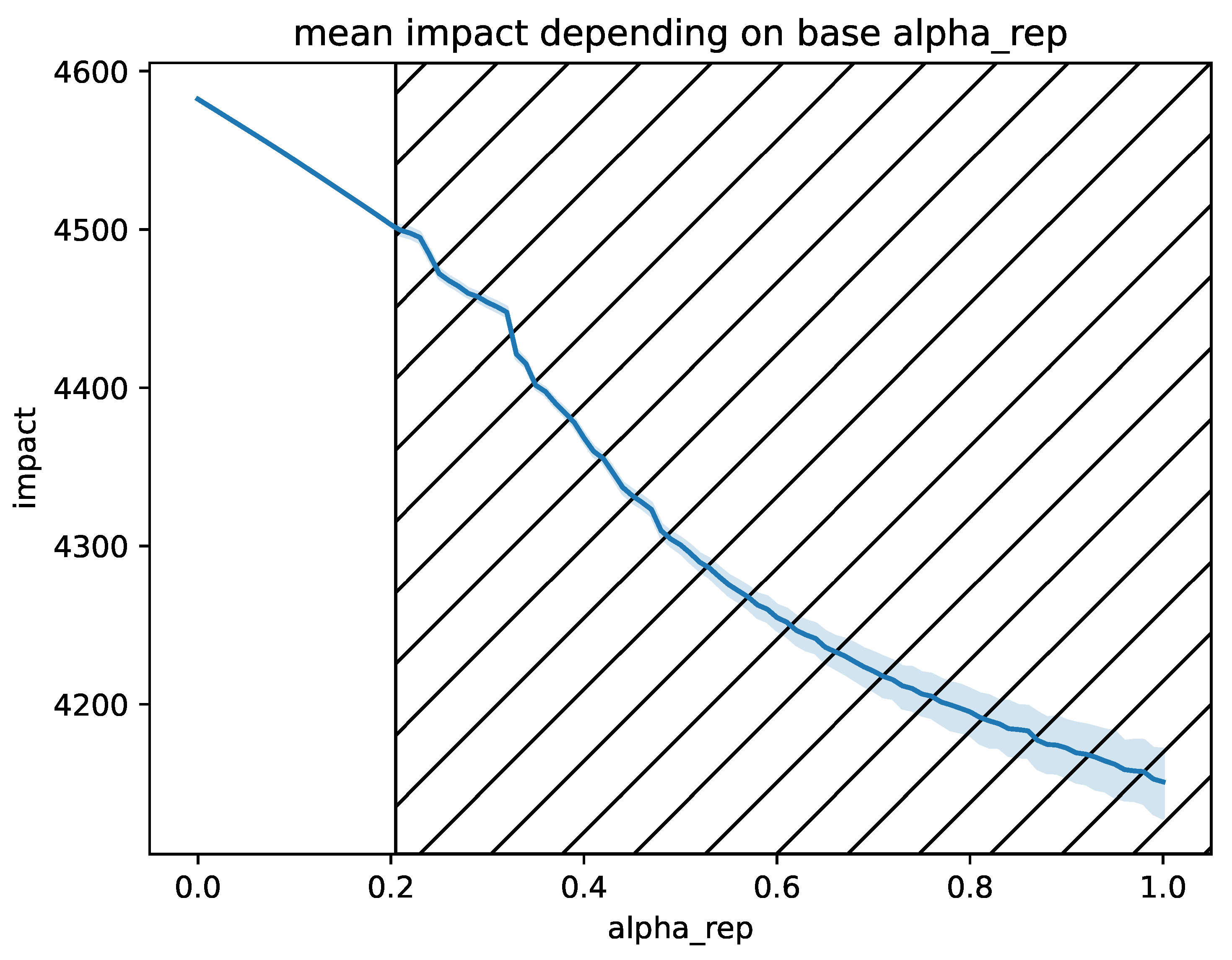
In our simulations, we have seen the sensibility of our carbon impact results to the parameters in Table 3. Indeed, the efficiency of the storage has a great impact on the system behavior. Hydrogen storage yields lower carbon emissions when its efficiency ${\eta }_{H_2}$ is higher than some threshold. The greater is ${\eta }_{H_2}$, the greater ${\alpha }_{rep}t$ could be and so the range for adapting ${\alpha }_{rep}t$ via learning is more important. 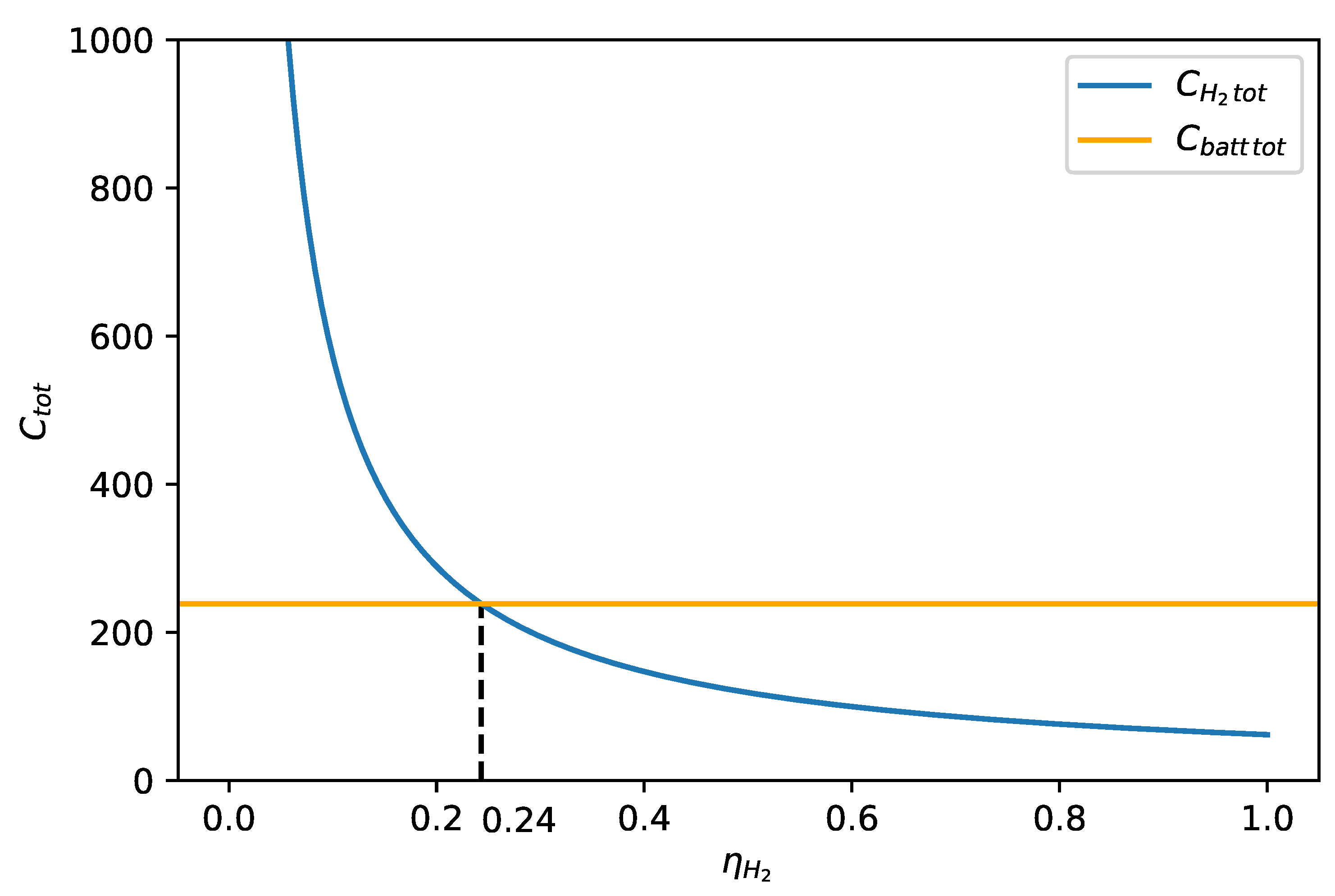To find the threshold in ${\eta }_{H_2}$, we first compute the total carbon intensity of storing one kW·h in a given storage, including the carbon intensity of energy production. For $H_2$, we obtain:

$$C_{H_{2}tot}=C_{H_{2}Out}+\frac{C_{H_{2}In}+C_{solar}}{{\eta }_{H_2}}{\mathrm{gCO}}_2\mathrm{eq}/\mathrm{kW}·\mathrm{h}$$

(63)

We display the value of (63) of both storages in Figure 5 with respect to ${\eta }_{H_2}$, the other parameters are taken from Table 3. When $C_{H_{2}tot}<C_{batttot}$ learning is useful since the policy must balance the lower carbon impact (using the hydrogen storage) with the low efficiency (using the battery storage). When $C_{H_{2}tot}>C_{batttot}$ the learned policy converges to ${\alpha }_{\mathbf{rep}}=\mathbf{0}$, as both objectives (minimizing the carbon impact and continuous powering of the datacenter) align.

Figure 5. The total hydrogen storage impact depending on the efficiency of storage.

We calculate from (63) and its battery variant, the threshold point where $C_{H_{2}tot}=C_{batttot}$ to be at efficiency:

$${\eta }_{H_2}^{*}=\frac{C_{H_{2}In}+C_{solar}}{C_{batttot}-C_{H_{2}Out}}$$

(64)

Using values in Table 3 on (64), hydrogen improves the carbon impact only when ${\eta }_{H_2}>{\eta }_{H_2}^{*}=0.24$. The current value is ${\eta }_{H_2}=0.35>0.24$, learning is also useful as shown in the simulations Table 4. We can also suggest that when the hydrogen storage efficiency will improve in the future, the impact of learning will be even more important.

6. Conclusions

We have addressed the problem of monitoring the hybrid energy storage of a partially islanded building with a goal of carbon impact minimization and self-consumption. We have reformulated the problem to reduce the number of components of the action to one, ${\alpha }_{rep}\left(t\right)$, the proportion of hydrogen storage given the building state ${\mathbf{s}}_t$. To learn the policy, ${\pi }_{\theta }:{\mathbf{s}}_t\to {\alpha }_{rep}\left(t\right)$, we propose a new DRL algorithm using a reward tailored to our problem, DDPG${\alpha }_{\mathbf{rep}}$. The simulation results show that when the hydrogen storage efficiency is large enough, learning of ${\alpha }_{rep}\left(t\right)$ allows a decrease to the carbon impact while lasting at least one year and maintaining $35\%$ of self-consumption. As hydrogen storage technologies improve, the proposed algorithm should have even more impact.

Learning the policy using the proposed DDPG${\alpha }_{\mathbf{rep}}$ can also be done when the storage model includes non-linearities. Learning can also adapt to climate changes in time using more recent data for learning. To measure such benefits, we will use in the future the ÉcoBioH2 real data to be measured in the sequel of the project. Learning from real data will reduce the gap between the model and the real system. Reducing this gap should improve performance. The proposed approach could also be used to optimize other environmental metrics with a multi-objective cost in $f({\mathbf{s}}_t,{\mathbf{a}}_t)$.

With our current formulation, policies cannot assess what day and hour it is as they only have two state variables to compute the hour: $E_{solar}\left(t\right)$ and $E_{building}\left(t\right)$. They cannot differentiate between 1 a.m. and 4 a.m. at night as those two times have the same consumption and no PV production. They also cannot differentiate between a cloudy summer and a clear winter as production and consumption are close in those two cases. In the future, we will consider taking into account the knowledge of the current time to enable the learned policy to adapt its behavior to the time of the day and month of the year.

Appendix A.1. When δE_storage(t) < 0

Using (28), (24) and its battery variant:

$$\begin{array}{cc}\hfill \delta E_{storage}\left(t\right)& \ge -E_{battinmax}-E_{H_{2}inmax}\hfill \end{array}$$

(A1)

Using (28), (23) and its battery variant:

$$\delta E_{storage}\left(t\right)\ge -\frac{E_{battmax}-E_{batt}(t-1)}{{\eta }_{batt}}-\frac{E_{H_{2}max}-E_{H_2}(t-1)}{{\eta }_{H_2}}$$

(A2)

Using (28), (23) and the battery variant of (24):

$$\begin{array}{cc}\hfill \delta E_{storage}\left(t\right)& \ge -E_{battinmax}-\frac{E_{H_{2}max}-E_{H_2}(t-1)}{{\eta }_{H_2}}\hfill \end{array}$$

(A3)

Using (28), (24) and the battery variant of (23):

$$\begin{array}{cc}\hfill \delta E_{storage}\left(t\right)& \ge -\frac{E_{battmax}-E_{batt}(t-1)}{{\eta }_{batt}}-E_{H_{2}inmax}\hfill \end{array}$$

(A4)

We obtain the global lower bound (41) by obtaining the min of (40), (A1)–(A4).

Appendix A.2. When δE_storage(t) > 0

Using (28), (25) and its battery variant:

$$\begin{array}{cc}\hfill \delta E_{storage}\left(t\right)& \le E_{batt}\left(t-1\right)+E_{H_2}\left(t-1\right)\hfill \end{array}$$

(A5)

Using (28), (26) and its battery variant:

$$\begin{array}{cc}\hfill \delta E_{storage}\left(t\right)& \le E_{battoutmax}+E_{H_{2}outmax}\hfill \end{array}$$

(A6)

Using (28), (25) and the battery variant of (26):

$$\begin{array}{cc}\hfill \delta E_{storage}\left(t\right)& \le E_{battoutmax}+E_{H_2}\left(t-1\right)\hfill \end{array}$$

(A7)

Using (28), (26) and the battery variant of (25):

$$\begin{array}{cc}\hfill \delta E_{storage}\left(t\right)& \le E_{batt}\left(t-1\right)+E_{H_{2}outmax}\hfill \end{array}$$

(A8)

We obtain the global upper bound (42) by obtaining the max of (A5)–(A8).

Appendix B.1. When δE_storage(t) > 0

Given (29) and (26)

$$\begin{array}{cc}\hfill {\alpha }_{rep}\left(t\right)& \le \frac{E_{H_{2}outmax}}{\delta E_{storage}\left(t\right)}\hfill \end{array}$$

(A9)

Given (29) and (25)

$$\begin{array}{cc}\hfill {\alpha }_{rep}\left(t\right)& \le \frac{E_{H_2}\left(t-1\right)}{\delta E_{storage}\left(t\right)}\hfill \end{array}$$

(A10)

From (30) and the battery variant of (26)

$$\begin{array}{cc}\hfill (1-{\alpha }_{rep}\left(t\right))\delta E_{storage}\left(t\right)& \le E_{battoutmax}\hfill \\ \hfill 1-{\alpha }_{rep}\left(t\right)& \le \frac{E_{battoutmax}}{\delta E_{storage}\left(t\right)}\hfill \\ \hfill 1-\frac{E_{battoutmax}}{\delta E_{storage}\left(t\right)}& \le {\alpha }_{rep}\left(t\right)\hfill \end{array}$$

(A11)

From (30) and the battery variant of (25)

$$\begin{array}{cc}\hfill (1-{\alpha }_{rep}\left(t\right))\delta E_{storage}\left(t\right)& \le E_{batt}\left(t-1\right)\hfill \\ \hfill 1-{\alpha }_{rep}\left(t\right)& \le \frac{E_{batt}\left(t-1\right)}{\delta E_{storage}\left(t\right)}\hfill \\ \hfill 1-\frac{E_{batt}\left(t-1\right)}{\delta E_{storage}\left(t\right)}& \le {\alpha }_{rep}\left(t\right)\hfill \end{array}$$

(A12)

Appendix B.2. When δE_storage(t) < 0

Given (31) and (24)

$$\begin{array}{cc}\hfill {\alpha }_{rep}\left(t\right)\delta E_{storage}\left(t\right)& \ge -E_{H_{2}inmax}\hfill \\ \hfill {\alpha }_{rep}\left(t\right)& \le -\frac{E_{H_{2}inmax}}{\delta E_{storage}\left(t\right)}\hfill \end{array}$$

(A13)

Given (31) and (23)

$$\begin{array}{cc}\hfill {\alpha }_{rep}\left(t\right)\delta E_{storage}\left(t\right)& \ge -\frac{E_{H_{2}max}-E_{H_2}\left(t-1\right)}{{\eta }_{H_2}}\hfill \\ \hfill {\alpha }_{rep}\left(t\right)& \le -\frac{E_{H_{2}max}-E_{H_2}\left(t-1\right)}{{\eta }_{H_2}\delta E_{storage}\left(t\right)}\hfill \end{array}$$

(A14)

From (30) and (24) battery variant

$$\begin{array}{cc}\hfill (1-{\alpha }_{rep}\left(t\right))\delta E_{storage}\left(t\right)& \ge -E_{battinmax}\hfill \\ \hfill 1-{\alpha }_{rep}\left(t\right)& \le \frac{-E_{battinmax}}{\delta E_{storage}\left(t\right)}\hfill \\ \hfill 1+\frac{E_{battinmax}}{\delta E_{storage}\left(t\right)}& \le {\alpha }_{rep}\left(t\right)\hfill \end{array}$$

(A15)

From (30) and (23) battery variant

$$\begin{array}{cc}\hfill (1-{\alpha }_{rep}\left(t\right))\delta E_{storage}\left(t\right)& \ge -\frac{E_{battmax}-E_{batt}\left(t-1\right)}{{\eta }_{batt}}\hfill \\ \hfill 1-{\alpha }_{rep}\left(t\right)& \le -\frac{E_{battmax}-E_{batt}\left(t-1\right)}{{\eta }_{batt}\delta E_{storage}\left(t\right)}\hfill \\ \hfill 1+\frac{E_{battmax}-E_{batt}\left(t-1\right)}{{\eta }_{batt}\delta E_{storage}\left(t\right)}& \le {\alpha }_{rep}\left(t\right)\hfill \end{array}$$

(A16)

We obtain the global upper bound (44) by obtaining the min of (A9) and (A10) when $\delta E_{storage}\left(t\right)>0$ and the max of (A13), (A14) when $\delta E_{storage}\left(t\right)<0$. We obtain the global lower bound (43) by obtaining the min of (A11) and (A12) when $\delta E_{storage}\left(t\right)>0$ and the max of (A15), (A16) when $\delta E_{storage}\left(t\right)<0$.