Abstract
Electricity supply quality (ESQ) is critical for healthy economic production, and regional differences in ESQ can widen economic development gaps. To contribute to a more equitable regional development, this study first develops a Gini index of ESQ distribution to measure the inequality among different cities. Then, an econometric model based on the Cobb–Douglas production function is established to quantify the effects of ESQ on regional economy. Finally, we estimate the impacts of ESQ improvement on reducing the economic inequality. The main results show that: (1) Substantial differences exist among the regional ESQ, and the national GDP-based ESQ Gini index was 0.720 in 2018. (2) A GDP-based Lorenz curve has a higher Gini coefficient than the population-based one does, while inequalities in cites are greater than those in rural areas. (3) The ESQ has significant impacts on the regional economic output, and a 1% reduction in the ESQ will, on average, reduce the city-level output by 0.142%. (4) ESQ improvement can significantly narrow the economic gap by up to 24.9%, that is, the ESQ Gini index of GDP distribution will decrease from 0.329 to 0.247 according to our scenario designs.
1. Introduction
Poverty eradication and sustainable energy supply are two of the 17 UN sustainable development goals (SDGs). High levels of asset or income inequality may hurt economic growth [1,2], and deficient power supply will also hinder economic development [3]. After the development in the past few decades, China has made remarkable achievements, with its GDP increasing from CNY 0.37 trillion in 1978 to CNY 91.93 trillion in 2018. However, the imbalance of regional development and inequality has been raising concerns from all walks of life. According to the data released by the National Bureau of Statistics of China, the Gini coefficient of per capita disposable income is 0.465 [4], while data from the China Household Finance Survey [5] indicate that the Gini coefficient is about 0.6. No matter which value is adopted, the Gini coefficient of China’s income is much higher than that of most peaceful countries, which reflects the inequality of distribution in China. Hence, narrowing the economic development gap between different regions is of great significance to the high-quality development of China’s economy.
Economic growth is positively affected by infrastructure assets, while income inequality declines with higher infrastructure quantity and quality [6]. The power system is an essential part of infrastructure and a lifeline for economic development, and the lack of resilient infrastructure harms firm productivity and even the whole society [7,8]. Resilient electricity supply is critical to economic development due to its significant role in attracting investment and employment, optimizing industrial structure, promoting economic production, as well as social stability, national security and food safety, and even the normal maintenance and operation of other infrastructure. The main ways that ESQ influences economic growth are as follows: First, electricity is a critical input in major manufacturing activities of urban production [9], which indicates that areas with poor ESQ have less chance to attract high value-added industries than those with high ESQ do. Second, production interruption cost, intermediate goods backlog cost and other additional costs will increase in the poor ESQ area. Additional direct cost such as losses in physical asset value and indirect cost such as supply chain disruption may incur under an unreliable power system [10]. Third, the regional and firm-level marginal costs to build backup generating power or own generation are very high when the ESQ is poor, and small-scale firms cost the highest proportion of investment to start up their own electricity facilities [11,12]. Thus, it is of great significance to estimate the impact of ESQ on economic development, which can provide a fresh perspective for bridging the regional development gap.
By the end of 2015, China had made great progress on electricity accessibility and the penetration rate of the access to electricity had reached 100%. However, the distribution of ESQ among regions is unequal, which may widen the regional economic gaps. Taking some major cities in China as an example, the System Average Interruption Duration Index (SAIDI), that is, the ratio of total outage time to the number of users, was less than 3 h per household in Foshan, Xiamen and Shenzhen in 2018. Meanwhile, the estimated SAIDI in Shanghai downtown area in 2020 was less than 5 min, reaching the first class like Tokyo and Singapore. By contrast, the SAIDI of Lhasa, the capital of the Tibet Autonomous Region, is more than 60 h per household, and the SAIDI of several areas in Xinjiang, Qinghai is more than 40 to 50 h. In March 2020, China put forward the policies of new infrastructure, aiming at promoting the construction of the power system, transport sector and other infrastructure. In this context, we can grasp the opportunity to enhance low ESQ regions in order to narrow the gap of economic development among different regions.
It is challenging to analyze the impact of ESQ on China’s economic development. First, city-level data of ESQ are relatively insufficient. The official city-level data, containing different ESQ indexes of 333 prefecture level cities, were only released in 2018. Second, the mechanism of ESQ affecting economic development is complex and the analysis of the ESQ impact on macroeconomics is relatively inadequate, compared with that on microeconomics or the productivity and behavior of firms. In addition, most research is concentrated in India or African countries, while the research about China is scarce. Considering the importance of China’s economic development and poverty eradication for the world economic development, this paper will evaluate the ESQ inequality among regions and discuss the impact mechanism of ESQ on regional output using cross-section data. Then, we will estimate the degree of inequality reduction in regional economic development after the ESQ improvement. The purpose of this study is to answer the following three questions:
- (1)
- What is the current situation of ESQ inequality among different regions in China?
- (2)
- How and to what degree does ESQ impact on China’s economic development?
- (3)
- If we improve the ESQ in appointed regions, how much will it narrow the regional economic development gap?
To answer the above three questions, we firstly introduce the Gini index to evaluate the ESQ inequality in China. Then, we develop an ESQ-adjusted Cobb–Douglas function to estimate the impact of ESQ on the regional economic output in China. Finally, we design three scenarios of ESQ improvement according to the regional policy documents in recent years. Therefore, this study contributes to the existing literature from the following two aspects. For one thing, there is no existing literature that introduces a proper tool to evaluate the ESQ inequality [13,14], thus we fill this void by introducing a mature economic tool, the Gini index, into the evaluation of the inequality of ESQ distribution for the first time, providing a more comparable indicator to measure the ESQ inequality. For another, most of the existing literature estimates the impact of ESQ or power outages on economic output from firm-level or industry-level perspectives [15], and our study aims to bridge this gap. On a macroscale, we introduce ESQ into the Cobb–Douglas function to illustrate the nexus between ESQ and economic output.
2. Literature Review
Energy is considered to be essential for well-being and development, and both quantity and quality matter a lot in economic development [8]. Among which, electricity is the lifeline and the backbone in modern economic development [8,16]. Most research focuses on the energy consumption–economic growth nexus [17,18,19], where the causal relationship between energy consumption and economic growth is still controversial [20,21,22]. However, there is scarce literature, compared with electricity consumption, focusing on the important role that ESQ plays in economic growth [9], and most of the existing studies quantify the reliability cost on different types of consumers [15,23] rather than on the macro economy. The positive relationship between ESQ and output has been tested by several studies. The authors in [24] use a parsimonious model and employ lightening density as an instrument to estimate the impact of outages on the economic growth of 39 countries in sub-Saharan Africa, indicating that a one percent increase in outages reduces long-run GDP per capita by 2.86%. A cross section analysis in 80 economies using World Bank Enterprise Surveys data suggests that power outages and electricity tariffs are negatively associated with firm-level productivity; especially, for a 1% increase in the total duration of power outages, productivity is expected to decrease by 0.10% at the firm level and by 0.07% at the industry level [25]. Limited studies focus on the ESQ of several cities in China, for instance, the Cobb–Douglas production function is used to quantify the impact of electric power outages in Shanghai from 1990 to 2006, combined with a model of the cost of electric energy unserved, which demonstrates that the unserved cost is about 1.81–10.26 CNY/kWh [26].
Inequality is another important issue concerned in social scientific research, which is usually discussed and analyzed in terms of income or some related monetary measure [27], as well as issues such as mortality, poverty and educational attainment [28,29,30]. More attention has been paid to the inequality of energy use recently [31,32]. It is important to note that, compared to the fact that a few measures have been taken to evaluate the inequality or unfairness of energy or electricity consumption, the assessment of the inequality of the distribution of electricity quality is scarce. Detailed reliability data displayed on graphs demonstrate that the reliability of electricity networks in different locations varies very significantly [14]. The authors in [33] formulate two indices, total energy curtailed (TEC) and curtailment unfairness index (CUI), using standard deviation of curtailed energies to quantify unfairness in the active power curtailment (APC) scheme. However, alternative indices such as the coefficient of variation and the Gini index used in the economic literature have not been applied to the area of the inequality of electricity reliability [13].
The Gini index has been widely used in inequality assessment in sociological and economical studies. The Gini index was initially used to measure the income or the wealth inequality. The Gini index was chosen for the relative income inequality measurement, and it was found that there is a strong effect of income inequality on burglary in the US [34]. An interesting study also implies that there is an inverse relationship between the income inequality measured by the Gini coefficient and the happiness explained by perceived fairness and general trust [35]. Researchers introduce the Lorenz curve and the Gini index into the measurements of inequality in the distribution of healthcare resources, length of life and the characteristics of infrastructure [36,37,38]. Lorenz curves and Gini coefficients are also applied to estimate the inequality of electricity consumption, helping to provide critical insights into the evolution of energy management in different states or countries. In addition, the Gini index has also been used to evaluate the inequality of the energy consumption in rural China, indicating a great disparity in energy inequality, and the decomposition of Gini coefficients shows that biomass contributes the most to the overall energy inequality [31]. Yet, there is no existing literature finding a good way to introduce the Lorenz curve and Gini index into the measurement of the quality of the electricity supply, which may be a critical part for developing countries.
3. Methodology and Data
3.1. Gini Index of ESQ Inequality
Before estimating the relationship between ESQ and economic output, we should first build an intuitive understanding of the inequality of ESQ distribution. The Gini index, or Gini coefficient, is generally used to measure the inequality of the distribution of income or expenditure. Some studies explore the Gini index to measure the inequality of the energy or electricity consumption [31,39]; however, few studies have used the Gini index to measure the inequality of ESQ. Since the Gini index has good characteristics in measuring ESQ [13], this paper tries to introduce the Gini index into the measurement of the inequality of ESQ in China.
In order to calculate the Gini index of ESQ, we need to obtain the Lorenz curve first. Generally, the Lorenz curve is obtained by ordering the variables on the vertical axis from the lowest to the highest value [31]. The author in [40] shows that ranking countries according to the ratio of y/x, that is, the ratio of local total outage time to the number of households or GDP in this paper, is necessary to obtain a properly shaped Lorenz curve and a well-defined Gini index. The local total outage time is calculated by multiplying SAIDI by the corresponding number of local households. It should be pointed out that the data object of SAIDI is for the users of a 10kV power supply system, which is different from the common concept of a household. Considering that the detailed data of electricity users are unavailable and China’s power penetration rate has reached 100%, we equate the number of electricity users with the number of households. In addition, as mentioned above, the indicators of ESQ include ESR, SAIDI and SAIFI. Considering that the Lorenz curve needs cumulative variables, we select SAIDI as a representative variable to display the Lorenz curve in this paper.
In this context, the ESQ Lorenz curve is displayed by the cumulative percentage of the outage time along the vertical axis versus the cumulative percentage of population or GDP on the horizontal axis, ranked by outage time per capita. A point on the ESQ Lorenz curve indicates that x% of the people or the economic output suffers y% of the electricity outages.
Obtaining a properly shaped ESQ Lorenz curve, we can then calculate the Gini index by Equation (1):
where denotes the cumulative percentage of population group or GDP group and is the cumulative percentage of outage time.
3.2. Estimation Model for the Impacts from ESQ to Economic Output
This paper introduces ESQ into the Cobb–Douglas production function to evaluate the impact of electricity reliability on economic output. The C-D production function has been used to estimate the contribution of each factor input to economic output. According to the different research fields, existing studies have added different factors into the C-D production function, such as human capital, energy consumption, efficiency, electricity outage, etc., to estimate the degree of impact of different factors on output [41,42,43,44].
Electricity is used in the production process of nearly every sector [45], such as health, food safety, economic failures, transport, etc. [46,47]. Access to high quality infrastructural services, such as electricity, is conducive to lower the marginal cost of information diffusion, trade, production, distribution and consumption of goods and services [44]. As a result, ESQ has a thorough influence on the economy and thus unreliable power supply will hinder economic development.
Next, we will discuss how to introduce ESQ into the production function. Several studies evaluate the negative impact of outage on economic output via TFP [8,48,49]; however, most of existing studies focus on the firm level and sector level. Assuming that low ESQ has a comprehensive negative impact on production activities because TFP such as institution and human capital cannot work well under a low ESQ situation and hence economic output decreases, we add an electricity-efficiency factor to the C-D production function and obtain an ESQ-adjusted Cobb–Douglas production function, as defined in Equation (2):
where is the total factor productivity (TFP), is the capital input, is the labor input, and and are the output elasticities of capital and labor, respectively.
The electricity-efficiency factor is determined by ESQ as:
where is a constant and is the output elasticity of , which is determined by electricity supply reliability rate , the System Average Interruption Duration Index (SAIDI) or the System Average Interruption Frequency Index (SAIFI) as in Equation (4):
Considering is usually presented as a percentage of , and and are interchangeable to embody , we set initially. Therefore, it could be expected that the output elasticity is negative.
Thus, the log form of the ESQ-adjusted Cobb–Douglas production function is specified as the benchmark regression equation:
where denotes a particular city, , , and are unknown parameters to be estimated, and is an error term. Limited by data availability, we estimate Equation (5) using cross-sectional data at the city level.
3.3. Data
The data used in the regression model and their sources are shown in Table 1. Prefecture-level output GDP, labor input and provincial-level fixed capital investment are from the China City Statistical Yearbook. Due to the lack of data, prefecture-level capital input K in the regression model is calculated by provincial-level Gross Domestic Fixed Capital Formation (GDFCF), multiplying the ratio of the prefecture-level fixed capital investment to the provincial-level one. Data of SAIDI and SAIFI are from the Power Reliability Index Report of Prefecture Level Cities (2018), Annual Report of National Power Reliability (2018) and the Getting Electricity data from Doing Business [50]. All the missing data are supplemented by the data from statistical yearbooks of provinces and cities or replaced by the average value of neighboring cities. All GDP and GDFCF data are adjusted according to the corresponding price reduction index. The Fourth National Economic Census (FNEC) was launched at the end of 2018 and some data have been adjusted according to the results of FNEC. However, some city-level data are unavailable, so we have to extrapolate them using previous years’ data. To make our data more comparable, this paper uses price deflators to adjust data, taking 2016 as the base year.

Table 1.
Data used in the regression.
In addition, the permanent resident population data used to calculate the Gini index in this paper are from city-level statistical yearbooks or the municipal Bureau of Statistics. Similarly, all the missing population data are supplemented by the average value of neighboring cities.
To obtain a better understanding of the data used in the regression, we have conducted a statistical analysis of the variables, see Table 2.
Table 2.
Summary statistics.
4. Results and Discussion
4.1. Measurement of ESQ Inequality among Different Regions
First, we display the difference of SAIDI and SAIFI among cities in China in 2018, as shown in Figure 1. It can be found that whether we assess ESQ by SAIDI or SAIFI, there are significant differences in ESQ among different regions of China. The ESQ in the southeast coast and other economically developed regions is significantly higher than that in other regions.
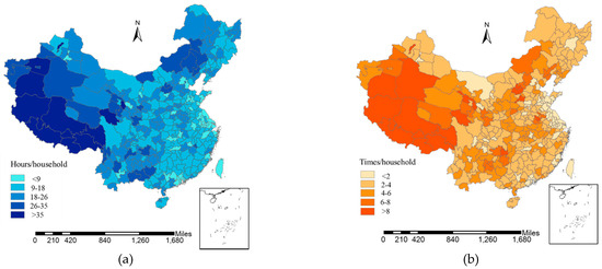
Figure 1.
(a) Distribution of SAIDI in China. (b) Distribution of SAIFI in China. Different ranks in the distribution maps are mainly based on the actual data and referenced by the planning of government’s requirements on the reliability of power grid over the years, for example, during the 11th five-year plan, the State Grid Corporation of China (SGCC) promised to promote the reliability rate of rural ESQ to 99.6%.
Then, we display Lorenz curves of SAIDI based on population and GDP standards, respectively, to manifest the inequality of ESQ distribution in China and calculate the Gini index, as shown in Figure 2. We can find that the Gini coefficients based on GDP are relatively larger, that is, the overall ESQ Lorenz curve based on the cumulative share of GDP has a 0.720 Gini index while the index of the cumulative population is 0.304, which indicates the great gap of ESQ among different economic groups. Comparing the inequality in urban areas with that in rural areas, the Gini coefficients in the former areas are much greater, which means the distribution of ESQ is more unequal in urban cities. This also confirms the fact that the news of the realization of high ESQ always appears in the core urban areas of big cities such as Shanghai and Beijing, while the ESQ in the suburban areas and urban-rural fringe of these cities is far from the same.
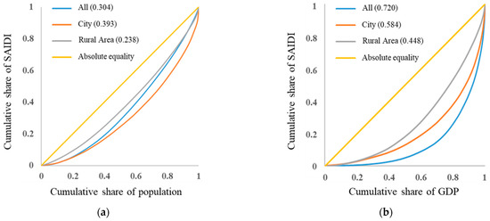
Figure 2.
Lorenz curves of ESQ (SAIDI) in China. (a) Lorenz curve with cumulative share of population on the horizontal axis. (b) Lorenz curve with cumulative share of GDP on the horizontal axis.
We also display Lorenz curves according to the different regional power grid companies, as shown in Figure 3. Again, we find that GDP-based ESQ inequality is much higher than the population-based one. The GDP-based Gini index is about 2.5 times larger than the population-based one in East China. Inner-region ESQ inequalities are significantly different among regions, for example, East China has the highest ESQ inequality with a GDP-based Gini coefficient of 0.733, meanwhile the Gini index of Northeast China is 0.355. The regional ESQ inequality implies the imbalanced development of the construction of the power system and unequal regional economic development.
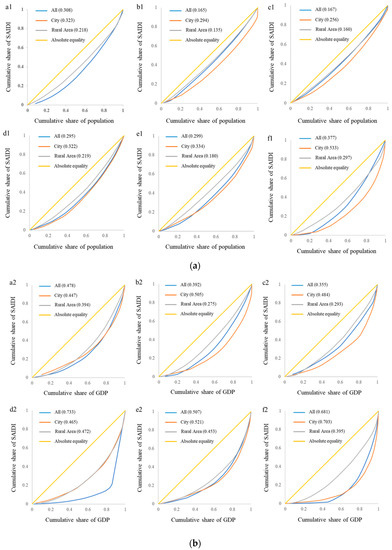
Figure 3.
Lorenz curve by regional power grid companies. (a) Lorenz curve with cumulative share of population on the horizontal axis. (b) Lorenz curve with cumulative share of GDP on the horizontal axis. Numbers 1–6 represent power grid companies in North China, Central China, Northeast China, East China, Northwest China and Southwest China, respectively.
Finally, we measured the internal inequality of ESQ distribution in different provinces, as shown in Figure 4. Two maps show that the degree of the internal ESQ inequality is significantly different among provinces. The internal inequality ESQ of Northwest China is relatively higher than that of East China. The GDP-based SAIFI inequality map shows a higher Gini coefficient rather than the population-based one. This result further indicates that the ESQ of cities with different economic development levels has great distinction. In general, the internal inequality in cities is much higher than that in rural areas, thus it can be considered to narrow the gap within and among cities.
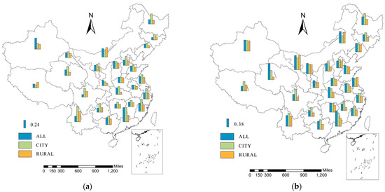
Figure 4.
Within-province inequality of ESQ distribution: (a) Population-based Gini coefficients of SAIFI. (b) GDP-based Gini coefficients of SAIFI.
4.2. The Impacts of ESQ on Regional Economic Output
4.2.1. Regression Results
The OLS regression results are shown in Table 3. SAIDI is incorporated into the benchmark regression model (4), named Model 1. All independent variables are significant at the 1% significance level and the sum of the parameters is also close to the assumption of constant returns to scale. The results of Model 1 show that every 1% reduction in ESQ will lead to a decline of 0.142% of the regional economic output on average. To initially measure the robustness of our regression results, we use another indicator that can be used to represent ESQ, SAIFI, to replace SAIDI in the regression model, obtaining Model 2 whose results are also significant. The results of Model 2 indicate that the deterioration of ESQ in every 1% will lead to a decline of 0.108% of the economic output, which is close to the above result. In a later section, we will further explore other auxiliary regression methods to ensure the robustness of our regression results.
Table 3.
Estimation results.
4.2.2. Regional Heterogeneity
China is in the stage of marketization reform of electricity power, and different regional electricity companies pay different attention to power supply quality due to different regional policies. In order to explore whether ESQ will vary among differentiated regional policies, we divide ESQ into groups according to different regional divisions of SGCC, as shown in Table 4. The results suggest that the parameters of ESQ in four of the six regions are significant, which indicates that generally ESQ has a negative effect on regional output in these regions. It should be noted that the parameters of ESQ of North China and Northwest China are not significant, which may be the result of the relatively small sample size of these two regions to the area so that those limited sample data cannot represent regional ESQ characteristics well and many data are regarded as outliers. The results of Central China and Northeast China indicate that ESQ may matter more than what our previous results show, and the impact of the ESQ on output is much deeper in these regions.
Table 4.
Regression results among different regions.
4.2.3. Trimmed Data for Robustness Test
We further use the robustness test to confirm the persuasiveness of the regression results, so as to ensure that the core parameters will not fluctuate sharply with the change in external conditions. We observe that the ESQ of some cities is much better or worse than that of other cities, so we trim 1% or 5% at each end of the data, respectively, and regress Model 1 again. The results of two trimmed data shown in Table 5 indicate that low ESQ has a significantly negative impact on economic output, which further proves the robustness of our previous OLS results.
Table 5.
OLS regression using trimmed data.
4.3. The Impacts of ESQ Improvement on Regional Inequality Gaps
In this section, we will discuss and analyze the effect of the improvement of ESQ on bridging the gap among regional economic development. We constructed three scenarios, as shown in Table 6. We obtain ESQ-improved GDP by comparing the ESQ of the past with the present one using the results of output elasticity of ESQ shown in Section 4.2.1 and Section 4.2.2. Again, we use SAIDI to represent ESQ here.
Table 6.
Scenario-based design of ESQ improvement.
China put forward the one belt, one road strategic development goal in late 2013. In 2015, China set the goal of alleviating poverty in an all-round way. They are the two most frequently used words in major government reports in recent years, where the key words of poverty alleviation policy have appeared 120 times and “One belt, one road” policy issues have appeared 70 times from 2013 to 2020. Although China has gotten rid of poverty by the end of 2020, the follow-up consolidation work is still in progress, which means that the Chinese government will attach great importance to these areas in the foreseeable future, and give preferential policies in these regions. In this context, it is of realistic significance to roughly estimate the extent to which the improvement of ESQ in these areas can promote the development of regional economy and further enhance the achievements of poverty alleviation, reducing the inequality of regional economic development.
Again, the Gini index is used to measure the effect of the improvement of ESQ on bridging the regional economic output gap. It is still controversial among the Gini indexes released by the official and university institutions in China, so they are not good references for this part. We calculate and compare the Gini index using GDP data before and after the ESQ improvement so that we can analyze the effect of ESQ improvement on reducing the economic inequality.
Based on the ESQ data in 2018 and the impact mechanism in Section 4.2, national Gini coefficients of GDP distribution under different scenarios are calculated based on the Lorenz curves with the cumulative percentage of GDP along the vertical axis and the cumulative percentage of population on the horizontal axis, as shown in Figure 5. The Gini coefficient of GDP distribution under three ESQ improvement scenarios is 0.247, 0.324 and 0.325, reduced by 24.9%, 1.52% and 1.22%, respectively, compared with the no-ESQ improvement scenario (benchmark in Figure 5). Compared with an annual average Gini decrease of 0.15% from 2003 to 2018 and an annual average Gini increase of 0.43% in the last three years according to Appendix B [55], we can confirm that the ESQ improvement can effectively bridge the regional economic gap.
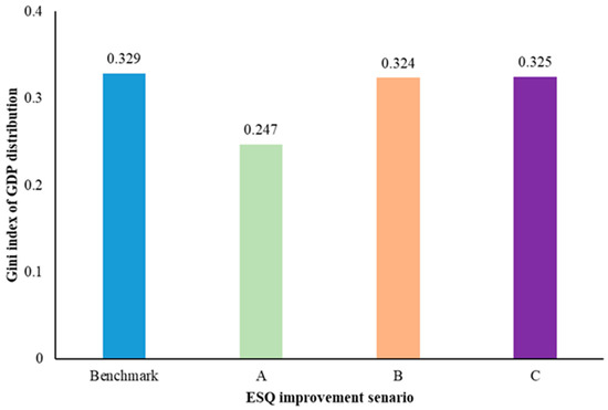
Figure 5.
The effect of ESQ improvement on narrowing regional economic gap.
5. Conclusions and Policy Implications
5.1. Conclusions
Electricity is the lifeline of economic development. However, unbalanced ESQ improvement strategies among regions and the large-scale application of renewable energy result in an enormous gap in the ESQ among cities in China. It is crucial to understand the state of ESQ inequality and the status and role of ESQ in the Chinese economy for reducing the regional economic gap. With this motivation, this study first introduced the Gini index to illustrate the inequality of the distribution of ESQ in China. Then, from a macro perspective, we built an ESQ-to-economic output model to estimate the impact of ESQ on the regional economy using cross-sectional data. Finally, based on the several frequently mentioned regional development policies by the Chinese government, we designed three possible ESQ improvement scenarios in the future and then calculated the effect on narrowing the economic gap.
The results indicate that the inequality of the distribution of ESQ in China is great, and the inequality among population groups varies significantly. The east coast enjoys much higher ESQ than the west coast of China does. Meanwhile, the higher Gini index based on GDP indicates the bias favor of the economically developed regions. Lorenz curves in six regions governed by different power grid companies indicate that within the regions, East China is the most unequally distributed region with the highest Gini index (0.733), while that within Northwest China is 0.355. The internal inequality in different provinces also indicates that the regions with more evenly distributed ESQ enjoy more balanced economic development.
Our econometrical model based on an augmented Cobb–Douglas production function verifies the negative impact of low ESQ on the regional economic output. The results show that every 1% decrease in ESQ (or 1% increase in SAIDI) leads to a decline of 0.142% of the regional economic output.
As to the effect of ESQ improvement on reducing the economic gap, the scenario design indicates that the regional economic gap can be narrowed up to 24.9%, with the Gini index of GDP decreasing from 0.329 to 0.247, 0.324, and 0.325, respectively.
Although we have answered several important questions about the inequality of ESQ distribution in China, there are limitations in this study and there is broad space for further research on the regional inequality of ESQ. First, with the improvement of information disclosure, more detailed panel data can be used to estimate the impact of ESQ on China’s economy more accurately. Second, more input variables, that is, the influence path of ESQ to economic output, such as the transportation industry, communication industry and manufacturing industry, can be given different weights for in-depth estimation when more data are available. Third, considering that the Gini index is introduced into the measurement of ESQ inequality for the first time, further comparison between the Gini index and other tools, such as standard deviation and coefficient of variance, and modeling optimization can be implemented in the future research. In addition, cost–benefit analysis can be used in the evaluation of the effect of ESQ improvement. The limitations in our study highlight the important directions for future research to reduce the economic gap in China by attaching importance to the ESQ.
5.2. Policy Implications
Although the Chinese government has made great efforts to develop the regional economy and to alleviate poverty, coordinating the development among regions and optimizing the industrial structure, inequality is still a big problem in China. Therefore, this paper tries to propose some policy implications on how to alleviate inequality from the perspective of improving ESQ based on the above discussions and conclusions.
First, it is an essential part of reducing the regional economic development to pay attention to the improvement of ESQ. Given that the demand for high ESQ is concentrated mainly in the cities of the eastern and central regions of China, low power supply quality areas should be paid more attention in the context of the construction of UHV power grids and ESQ improvement. Meanwhile, according to the actual development demand in different regions, the improvement degree of ESQ should be different among different regions. With the gradual deepening of China’s western development, the ESQ in central and western regions should be gradually improved. With the ESQ improved in the future, the inequality of ESQ among regions may slow down, showing the Kuznets process.
Second, with the growth of power demand and the use of clean energy, technologies and other supporting policies to ensure high-quality electricity supply need to be designed and implemented. Some cities in China have encountered the problem of electricity shortage because stable coal-fired power is gradually withdrawing with China’s goal of achieving carbon neutrality before 2060, thus high ESQ needs to be guaranteed by technologies such as demand side management, electricity storage, and microgrids, and relevant policy design needs to be further improved as well.
Author Contributions
Conceptualization, B.Z.; methodology, B.Z.; software, B.Z.; validation, B.Z., M.W.; formal analysis, B.Z.; investigation, B.Z.; resources, B.Z., M.W.; data curation, B.Z.; writing—original draft preparation, B.Z.; writing—review and editing, B.Z., M.W.; visualization, B.Z., M.W.; supervision, B.Z.; project administration, B.Z. All authors have read and agreed to the published version of the manuscript.
Funding
This research received no external funding.
Institutional Review Board Statement
Not applicable.
Informed Consent Statement
Not applicable.
Data Availability Statement
Data will be available on request.
Acknowledgments
The authors would like to acknowledge the contribution of all partners for their participation and ideas during the development of this article. The authors would also like to extend a special thanks to the editor and the anonymous reviewers for their constructive comments and suggestions, which improved the quality of this article.
Conflicts of Interest
The authors declare no conflict of interest.
Abbreviations
ESQ—electricity supply quality; SDGs—sustainable development goals; SAIDI—the System Average Interruption Duration Index; SAIFI—the System Average Interruption Frequency Index; TFP—total factor productivity; ESR—electricity supply reliability rate; GDFCF—Gross Domestic Fixed Capital Formation.
Appendix A
Table A1.
List of the 832 national-level poor counties.
Table A1.
List of the 832 national-level poor counties.
| Province | Number of Poverty Counties | Names of Poverty Counties |
|---|---|---|
| Anhui | 20 | Yuexi, Shou, Qianshan, Susong, Yingshang, Dangshan, Lingbi, Si, Yu’an, Shucheng, Lixin, Taihu, Shitai, Funan, Xiao, Huoqiu, Wangjiang, Linquan, Jinzhai, Yingdong |
| Chongqing | 14 | Wanzhou, Qianjiang, Wulong, Fengdu, Xiushan, Kaizhou, Yunyang, Wushan, Fengjie, Shizhu, Chengkou, Pengshui, Youyang, Wuxi |
| Gansu | 58 | Gaolan, Kongtong, Zhengning, Liangdang, Linxia, Hezuo, Yongdeng, Yuzhong, Jingtai, Gangu, Wushan, Jingchuan, Lingtai, Cheng, Hui, Zhuoni, Diebu, Maqu, Luqu, Xiahe, Wen, Wudu, Kang, Lintan, Zhouqu, Jishishan, Yongjing, Guanghe, Hezheng, Kangle, Maiji, Zhangjiachuan, Qin’an, Qingshui, Zhuanglang, Jingning, Heshui, Huachi, Ning, Qingcheng, Lintao, Anding, Longxi, Zhang, Weiyuan, Huining, Jingyuan, Gulang, Tianzhu, Huan, Dangchang, Xihe, Li, Dongxiang, Linxia, Zhengyuan, Tongwei, Min |
| Guangxi | 33 | Longzhou, Longsheng, Ziyuan, Tianyang, Tiandong, Xilin, Fuchuan, Jinxiu, Ningming, Daxin, Huanjiang, Rongan, Longan, Shanglin, Lingyun, Tianlin, Xincheng, Mashan, Debao, Donglan, Fengshan, Bama, Jingxi, Zhaoping, Tiandeng, Longlin, Rongshui, Luocheng, Leye, Napo, Dahua, Sanjiang, Duan |
| Guizhou | 66 | Chishui, Tongxin, Fenggang, Meitan, Xishui, Xixiu, Pingba, Qianxi, Bijiang, Wanshan, Jiangkou, Yuping, Xingren, Wengan, Longli, Liuzhi, Panzhou, Daozhen, Wuchuan, Puding, Zhenning, Dafang, Shiqian, Yinjiang, Anlong, Shibing, Sansui, Zhenyuan, Leishan, Majiang, Danzhai, Guiding, Huishui, Puan, Zhenfeng, Guanling, Songtao, Sinan, Dejiang, Changshun, Dushan, Pingtang, Libo, Cengong, Tianzhu, Taijiang, Huangping, Liping, Qixingguan, Zhijin, Jinping, Luodian, Zhengan, Ceheng, Jianhe, Shuicheng, Sandu, Ziyun, Wangmo, Congjiang, Qinglong, Yanhe, Rongjiang, Hezhang, Nayong, Weining |
| Hainan | 5 | Baoting, Qiongzhong, Wuzhishan, Lingao, Baisha |
| Hebei | 45 | Haixing, Nanpi, Wangdu, Pingshan, Qinglong, Weixian, Pingxiang, Wei, Yi, Pingquan, Yanshan, Wuyi, Raoyang, Fucheng, Xingtang, Lingshou, Zanhuang, Daming, Lincheng, Julu, Xinhe, Guangzong, Laishui, Tang, Quyang, Shunping, Xuanhua, Wanquan, Chongli, Chengde, Luanping, Wuqiang, Weichang, Longhua, Fengning, Fuping, Laiyuan, Zhangbei, Shangyi, Wei, Huaian, Chicheng, Guyuan, Kangbao, Yangyuan |
| Heilongjiang | 20 | Gannan, Fuyu, Raohe, Fuyuan, Wangkui, Longjiang, Tailai, Kedong, Suibin, Huanan, Huachuan, Tangyuan, Tongjiang, Lanxi, Mingshui, Gangang, Baiquan, Hailun, Lindian, Yanshou |
| Henan | 38 | Lankao, Hua, Xin, Shenqiu, Xincai, Luanchuan, Yiyang, Luoning, Fengqiu, Zhenping, Neixiang, Minquan, Sui, Ningling, Zhecheng, Yucheng, Guangshan, Shangcheng, Gushi, Huangchuan, Shangshui, Dancheng, Huaiyang, Taikang, Song, Ruyang, Lushan, Fan, Taiqian, Lushi, Nanzhao, Xichuan, Tongbai, Sheqi, Huaibin, Shangcai, Pingyu, Queshan |
| Hubei | 28 | Hongan, Shennongjia, Yangxin, Danjiangkou, Zigui, Baokang, Tuanfeng, Luotian, Yingshan, Xuanen, Laifeng, Hefeng, Yunyang, Yunxi, Zhuxi, Zhushan, Fang, Changyang, Wufeng, Xiaochang, Dawu, Macheng, Qichun, Enshi, Lichuan, Jianshi, Xianfeng, Badong |
| Hunan | 40 | Chaling, Yanling, Shimen, Guidong, Zhongfang, Xinshao, Suining, Wugang, Pingjiang, Cili, Anhua, Yizhang, Rucheng, Anren, Jianghua, Chenxi, Hetong, Xinhuang, Zhijiang, Jingzhou, Sangzhi, Luxi, Fenghuang, Huayuan, Baojing, Guzhang, Yongshun, Tongdao, Mayang, Xupu, Yuanling, Xinning, Shaoyang, Longhui, Dongkou, Chengbu, Xinhua, Lianyuan, Longshan, Xintian |
| Inner Mongolia | 31 | Linxi, Wuchuan, Balinyou banner, Kalaqin banner, Ningcheng, Horqin Left Wing Back banner, Chahar Right Wing Back Banner, Arshan, Jalaid Banner, Horqin Right Wing Middle Banner, Sonid Right Banner, Oroqen, Molidava Banner, Tuquan, Horqin Right Front Banner, Horqin Left Middle Banner, Kulun flag, Naiman Banner, Ar Horqin Banner, Ongniud Banner, Aohan Banner, Bairin Left Banner, Zhengxiangbai Banner, Taibus Banner, Zhuozi, Chahar Right Front Banner, Shangdu, Xinghe, Chahar Right Middle Banner, Siziwang Banner, Huade |
| Jiangxi | 24 | Jinggangshan, Jian, Ruijin, Wanan, Yongxin, Guangchang, Shangrao, Hengfeng, Lianhua, Shangyou, Anyuan, Huichang, Xunwu, Shicheng, Nankang, Suichuan, Lean, Yugan, Xingguo, Yudu, Ningdu, Ganxian, Boyang, Xiushui |
| Jilin | 8 | Zhenlai, Longjing, Helong, Jingyu, Tongyu, Wangqing, Antu, Da’an |
| Ningxia | 8 | Yanchi, Longde, Jingyuan, Pengyang, Tongxin, Yuanzhou, Haiyuan, Xiji |
| Qinghai | 42 | Tongde, Henan, Dulan, Pingan, Xunhua, Gangcha, Golmud, Delingha, Wulan, Tianjun, Datong, Huangzhong, Huangyuan, Huzhu, Menyuan, Qilian, Haiyan, Xinghai, Guinan, Maduo, Yushu, Chindu, Ledu, Minhe, Hualong, Jianzha, Tongren, Zeku, Gonghe, Guide, Jiuzhi, Maqin, Banma, Zhidoi, Zadoi, QumarlêumaNangqian, Gande, Dari, Lenghu, Mangya, Dachaidan |
| Shaanxi | 56 | Yanchang, Foping, Hengshan, Dingbian, Zhouzhi, Yijun, Fufeng, Longxian, Qianyang, Linyou, Taibai, Yongshou, Changwu, Xunyi, Chunhua, Heyang, Chengcheng, Pucheng, Fuping, Yanchuan, Yichuan, Liuba, Suide, Mizhi, Wubao, Zhenping, Zhenan, Yintai, Yaozhou, Baishui, Jiaxian, Qingjian, Zizhou, Nanzheng, Chenggu, Yangxian, Xixiang, Mianxian, Ningqiang, Zhenba, Hanbin, Ziyang, Baihe, Ningshan, Lueyang, Xunyang, Pingli, Shiquan, Hanyin, Langao, Shangzhou, Luonan, Danfeng, Shangnan, Shanyang, Zhashui |
| Shanxi | 36 | Youyu, Jixian, Zhongyang, Loufan, Yanggao, Lingqiu, Yunzhou (Datong), Wuxiang, Zuoquan, Heshun, Pinglu, Fanshi, Shenchi, Wuzhai, Kelan, Hequ, Baode, Xixian, Lanxian, Fangshan, Guangling, Hunyuan, Tianzhen, Wutai, Huguan, Ningwu, Jingle, Pianguan, Xingxian, Pingshun, Yonghe, Daning, Fenxi, Shilou, Linxian, Daixian |
| Sichuan | 66 | Nanbu, Guangan, Beichuan, Muchuan, Jialing, Yilong, Bazhou, Wenchuan, Lixian, Maoxian, Maerkang, Luding, Pingwu, Zhaohua, Chaotian, Qingchuan, Langzhong, Nanjiang, Songpan, Jiuzhaigou, Jinchuan, Xiaojin, Ruoergai, Hongyuan, Kangding, Danba, Jiulong, Xiangcheng, Daocheng, Cangxi, Wangcang, Jiange, Xuanhan, Wanyuan, Pingchang, Tongjiang, Xuyong, Gulin, Mabian, Pingshan, Aba, Rangtang, Heishui, Seda, Shiqu, Litang, Dege, Ganzi, Xinlong, Yajiang, Luhuo, Derong, Daofu, Batang, Baiyu, Leibo, Ganluo, Yanyuan, Muli, Meigu, Butuo, Zhaojue, Jinyang, Xide, Yuexi, Puge |
| Tibet | 74 | Chengguan, Yadong, Naidong, Bayi, Karuo, Lhünzhub, Damxung, Nyêmo, Qushui, DoilungdêoilunDagzêagMaizhokunggar, RiwoqêiwoqnqêqwoSangri, Qonggyai, Qusum, Lhozhag, Gyaca, Cona, Bainang, Kangmar, DinggyêinGyirong, Nyalam, Biru, Gar, Gongbujiangda, Mainling, BomêomJomda, Lhorong, Bianba, Zhanang, Konka, Comai, LhünzêzLNagarzêagSangzhuzi, Tingri, Ngamring, Rinbung, Zhongba, Kamba, Lhari, Nyainrong, Anduo, Sog, Bange, Purang, Zanda, Rutog, Medog, Zayüayay, ZaNamling, Saga, Lazi, GyangzêyaXietongmen, Sa’gya, Gonjo, Chagyab, Markam, Zuogong, Basu, Naqu, Baqing, Shenzha, Nyima, Shuanghu, GarzêzGCoqen, Gengya |
| Xinjiang | 32 | Minfeng, Qapqal Xibe, Qinghe, Tuoli, Barkoi, Nilka, Jeminay, Akqi, Wuqia, Zepu, Hetianxian, Hetian, Yuepuhu, Shule, Shufu, Bachu, Kashgar, Makit, Tajik, Artux, Wushi, Kalpin, Pishan, Luopu, Qira, Karakax, Yutian, Yecheng, Payzawat, Yengisar, Yarkant, Aketao |
| Yunan | 88 | Xundian, Luoping, Yulong, Ninger, Yunxian, Mouding, Yaoan, Shiping, Menghai, Xiangyun, Binchuan, Weishan, Eryuan, Heqing, Mang, Dongchuan, Luquan, Shizong, Fuyuan, Longling, Changning, Suijiang, Weixin, Jinggu, Zhenyuan, Menglian, Ximeng, Linxiang, Fengqing, Zhenkang, Shuangjiang, Gengma, Cangyuan, Shuangbai, Nanhua, Dayao, Yongren, Luxi, Yanshan, Xichou, Mengla, Yangbi, Nanjian, Yongping, Yingjiang, Longchuan, Shangri-La, Deqin, Xuanwei, Shidian, Longyang, Yanjin, Ludian, Zhaoyang, Daguan, Yiliang, Yongshan, Qiaojia, Yongsheng, Jingdong, Mojiang, Jiangcheng, Yongde, Wuding, Honghe, Luchun, Jinping, Wenshan, Malipo, Maguan, Qiubei, Funing, Midu, Yuanyang, Yunlong, Jianchuan, Lianghe, Gongshan, Weixi, Jinze, Zhenxiong, Ninglang, Lancang, Pingbian, Guangnan, Lushui, Fugong, Lanping |
| Total | 832 | - |
Appendix B
Table A2.
National Gini coefficients of per capita disposable income.
Table A2.
National Gini coefficients of per capita disposable income.
| Year | Gini Coefficient |
|---|---|
| 2003 | 0.479 |
| 2004 | 0.473 |
| 2005 | 0.485 |
| 2006 | 0.487 |
| 2007 | 0.484 |
| 2008 | 0.491 |
| 2009 | 0.49 |
| 2010 | 0.481 |
| 2011 | 0.477 |
| 2012 | 0.474 |
| 2013 | 0.473 |
| 2014 | 0.469 |
| 2015 | 0.462 |
| 2016 | 0.465 |
| 2017 | 0.467 |
| 2018 | 0.468 |
References
- Cingano, F. Trends in Income Inequality and Its Impact on Economic Growth; OECD Social, Employment and Migration Working Papers; OECD: Paris, France, 2014; pp. 1–64. [Google Scholar] [CrossRef]
- Deininger, K.; Olinto, P. Asset Distribution, Inequality, and Growth; The World Bank: Washington, DC, USA, 1999; pp. 1–19. [Google Scholar]
- Jones, C.I. Intermediate goods and weak links in the theory of economic development. Am. Econ. J. Macroecon. 2011, 3, 1–28. [Google Scholar] [CrossRef]
- NBS. China Statistical Yearbook. Available online: http://www.stats.gov.cn/ (accessed on 20 April 2021).
- CHFS; Survey and Research Center for China Household Finance. China Household Finance Survey, CHFS. Available online: https://chfs.swufe.edu.cn/ (accessed on 20 April 2021).
- Calderón, C.; Servén, L. The Efects of Infrastructure Development on Growth and Income Distribution; The World Bank: Washington, DC, USA, 2004; pp. 1–42. [Google Scholar]
- Escribano, A.; Guasch, J.L.; Pena, J. Assessing the Impact of Infrastructure Constraints on Firm Productivity in Africa. Cross-Country Comparisons Based on Investment Climate Surveys from 1999 to 2005; Working Paper 09-86; Economic Series; Departamento de Economia Universidad Carlos III de Madrid: Madrid, Spain, 2009; pp. 11–27. [Google Scholar]
- Hallegatte, S.; Rentschler, J.; Rozenberg, J. Lifelines: The Resilient Infrastructure Opportunity; The World Bank: Washington, DC, USA, 2019; pp. 2–137. [Google Scholar]
- Gertler, P.J.; Lee, K.; Mobarak, A.M. Electricity Reliability and Economic Development in Cities: A Microeconomic Perspective; EEG State-of-Knowledge Paper Series; University of California: Berkeley, CA, USA, 2017; pp. 4–12. [Google Scholar]
- Wenzel, L.; Wolf, A. Protection against Major Catastrophes: An Economic Perspective; HWWI Research Paper; Hamburg Institute of International Economics (HWWI): Hamburg, Germany, 2013; pp. 5–12. [Google Scholar]
- Adenikinju, A.F. Analysis of the Cost of Infrastructure Failures in a Developing Economy: The Case of the Electricity Sector in Nigeria; AERC Research Paper 148; African Economic Research Consortium: Nairobi, Kenya, 2005; pp. 1–31. [Google Scholar]
- Foster, V.; Steinbuks, J. Paying the Price for Unreliable Power Supplies: In-House Generation of Electricity by Firms in Africa; The World Bank: Washington, DC, USA, 2009; pp. 1–26. [Google Scholar]
- Heylen, E.; Ovaere, M.; Proost, S.; Deconinck, G.; Van Hertem, D. Fairness and inequality in power system reliability: Summarizing indices. Electr. Power Syst. Res. 2019, 168, 313–323. [Google Scholar] [CrossRef]
- Strbac, G.; Kirschen, D.; Moreno, R. Reliability Standards for the Operation and Planning of Future Electricity Networks; Now Foundations and Trends: Delft, The Netherlands, 2016; pp. 175–176. [Google Scholar]
- Chen, H.; Chen, X.; Niu, J.; Xiang, M.; He, W.; Küfeoğlu, S. Estimating the marginal cost of reducing power outage durations in China: A parametric distance function approach. Energy Policy 2021, 155, 112366. [Google Scholar] [CrossRef]
- Chen, H.; Liu, S.; Liu, Q.; Shi, X.; Wei, W.; Han, R.; Küfeoğlu, S. Estimating the impacts of climate change on electricity supply infrastructure: A case study of China. Energy Policy 2021, 150, 112119. [Google Scholar] [CrossRef]
- Tang, C.F.; Tan, B.W.; Ozturk, I. Energy consumption and economic growth in Vietnam. Renew. Sustain. Energy Rev. 2016, 54, 1506–1514. [Google Scholar] [CrossRef]
- Adhikari, D.; Chen, Y. Energy consumption and economic growth: A panel cointegration analysis for developing countries. Rev. Econ. Financ. 2013, 3, 68–80. [Google Scholar]
- Ocal, O.; Aslan, A. Renewable energy consumption—Economic growth nexus in Turkey. Renew. Sustain. Energy Rev. 2013, 28, 494–499. [Google Scholar] [CrossRef]
- Zhang, W.; Yang, S. The influence of energy consumption of China on its real GDP from aggregated and disaggregated viewpoints. Energy Policy 2013, 57, 76–81. [Google Scholar] [CrossRef]
- Zhang, X.-P.; Cheng, X.-M. Energy consumption, carbon emissions, and economic growth in China. Ecol. Econ. 2009, 68, 2706–2712. [Google Scholar] [CrossRef]
- Lee, C.-C.; Chang, C.-P. Energy consumption and economic growth in Asian economies: A more comprehensive analysis using panel data. Resour. Energy Econ. 2008, 30, 50–65. [Google Scholar] [CrossRef]
- Hashemi, M.; Jenkins, G.P.; Jyoti, R.; Ozbafli, A. Evaluating the cost to industry of electricity outages. Energy Sources Part B Econ. Plan. Policy 2018, 13, 340–349. [Google Scholar] [CrossRef]
- Andersen, T.B.; Dalgaard, C.-J. Power outages and economic growth in Africa. Energy Econ. 2013, 38, 19–23. [Google Scholar] [CrossRef]
- Arlet, J. Electricity Tariffs, Power Outages and Firm Performance: A Comparative Analysis. In Proceedings of the DECRG Kuala Lumpur Seminar Series, Kuala Lumpur, Malaysia, 19 March 2017; pp. 1–41. [Google Scholar]
- Sun, T.; Wang, X.; Ma, X. Relationship between the economic cost and the reliability of the electric power supply system in city: A case in Shanghai of China. Appl. Energy 2009, 86, 2262–2267. [Google Scholar] [CrossRef]
- Pachauri, S. Energy Inequality. 2014. Available online: https://iiasa.ac.at/web/home/research/alg/energy-inequality.html (accessed on 20 April 2021).
- Ahluwalia, M.S. Inequality, poverty and development. J. Dev. Econ. 1976, 3, 307–342. [Google Scholar] [CrossRef]
- Duncan, G.J.; Murnane, R.J. Whither Opportunity? Rising Inequality, Schools, and Children’s Life Chances; Russell Sage Foundation: New York, NY, USA, 2011; pp. 1–534. [Google Scholar]
- Lynch, J.W.; Smith, G.D.; Kaplan, G.A.; House, J.S. Income inequality and mortality: Importance to health of individual income, psychosocial environment, or material conditions. BMJ 2000, 320, 1200–1204. [Google Scholar] [CrossRef]
- Wu, S.; Zheng, X.; Wei, C. Measurement of inequality using household energy consumption data in rural China. Nat. Energy 2017, 2, 795–803. [Google Scholar] [CrossRef]
- Bianco, V.; Cascetta, F.; Marino, A.; Nardini, S. Understanding energy consumption and carbon emissions in Europe: A focus on inequality issues. Energy 2019, 170, 120–130. [Google Scholar] [CrossRef]
- Latif, A.; Gawlik, W.; Palensky, P. Quantification and mitigation of unfairness in active power curtailment of rooftop photovoltaic systems using sensitivity based coordinated control. Energies 2016, 9, 436. [Google Scholar] [CrossRef]
- Choe, J. Income inequality and crime in the United States. Econ. Lett. 2008, 101, 31–33. [Google Scholar] [CrossRef]
- Oishi, S.; Kesebir, S.; Diener, E. Income inequality and happiness. Psychol. Sci. 2011, 22, 1095–1100. [Google Scholar] [CrossRef]
- Woldemichael, A.; Takian, A.; Sari, A.A.; Olyaeemanesh, A. Inequalities in healthcare resources and outcomes threatening sustainable health development in Ethiopia: Panel data analysis. BMJ Open 2019, 9, e022923. [Google Scholar] [CrossRef]
- Shkolnikov, V.M.; Andreev, E.E.; Begun, A.Z. Gini coefficient as a life table function: Computation from discrete data, decomposition of differences and empirical examples. Demogr. Res. 2003, 8, 305–358. [Google Scholar] [CrossRef]
- Hörcher, D.; Graham, D.J. The Gini index of demand imbalances in public transport. Transportation 2020. [Google Scholar] [CrossRef]
- Lawrence, S.; Liu, Q.; Yakovenko, V.M. Global inequality in energy consumption from 1980 to 2010. Entropy 2013, 15, 5565–5579. [Google Scholar] [CrossRef]
- Groot, L. Carbon lorenz curves. Resour. Energy Econ. 2010, 32, 45–64. [Google Scholar] [CrossRef]
- Breton, T.R. Can institutions or education explain world poverty? An augmented Solow model provides some insights. J. Socio Econ. 2004, 33, 45–69. [Google Scholar] [CrossRef]
- Fang, Y. Economic welfare impacts from renewable energy consumption: The China experience. Renew. Sustain. Energy Rev. 2011, 15, 5120–5128. [Google Scholar] [CrossRef]
- Ibragimov, Z.; Vasylieva, T.A.; Liulov, O.V. The national economy competitiveness: Effect of macroeconomic stability, renewable energy on economic growth. In Proceedings of the Socio Economic Problems of Sustainable Development—37th International Scientific Conference on Economic and Social Development, Baku, Azerbaijan, 14–15 February 2019; pp. 878–887. [Google Scholar]
- Mensah, J.T. Bring back our light: Power outages and industrial performance in sub-Saharan Africa. In Proceedings of the AAEA 2016 Annual Meeting, Boston, MA, USA, 31 July–2 August 2016; pp. 1–28. [Google Scholar]
- World Bank. World Development Report 1994: Infrastructure for Development; Oxford University Press: New York, NY, USA, 1994; pp. 252–257. [Google Scholar]
- Matthewman, S.; Byrd, H. Blackouts: A Sociology of Electrical Power Failure. Social Space 2013, 6, 1–25. [Google Scholar]
- World Bank Group. State of Electricity Access Report 2017 (Vol. 2): Full Report (English). Available online: http://documents.worldbank.org/curated/en/364571494517675149/full-report (accessed on 20 April 2021).
- Ackah, C.G.; Asuming, P.O.; Abudu, D. Misallocation of Resources and Productivity: The Case of Ghana; Institute of Statistical, Social and Economic Research, University of Ghana: Accra, Ghana, 2018; pp. 1–20. [Google Scholar]
- Fisher-Vanden, K.; Mansur, E.T.; Wang, Q.J. Costly Blackouts? Measuring Productivity and Environmental Effects of Electricity Shortages; 0898-2937; National Bureau of Economic Research: Cambridge, MA, USA, 2012; pp. 1–29. [Google Scholar]
- Doing Business. Getting Electricity. Available online: https://www.doingbusiness.org/en/data/exploretopics/getting-electricity (accessed on 27 May 2021).
- NBS. China City Statistical Yearbook. Available online: http://www.stats.gov.cn/ (accessed on 20 April 2021).
- NBS. Statistical Yearbook of the Chinese Investment in Fixed Assets. Available online: http://www.stats.gov.cn/ (accessed on 20 April 2021).
- NEA. Power Reliability Index Report of Prefecture Level Cities. Available online: http://www.nea.gov.cn/ (accessed on 20 April 2021).
- NEA. Annual Report of National Power Reliability. Available online: http://www.nea.gov.cn/ (accessed on 20 April 2021).
- NBS. China Yearbook of Household Survey. Available online: http://www.stats.gov.cn/ (accessed on 20 April 2021).
Publisher’s Note: MDPI stays neutral with regard to jurisdictional claims in published maps and institutional affiliations. |
© 2021 by the authors. Licensee MDPI, Basel, Switzerland. This article is an open access article distributed under the terms and conditions of the Creative Commons Attribution (CC BY) license (https://creativecommons.org/licenses/by/4.0/).