Abstract
Digital rock physics is an often-mentioned approach to better understand and model transport processes occurring in tight nanoporous media including the organic and inorganic matrix of shale. Workflows integrating nanometer-scale image data and pore-scale simulations are relatively undeveloped, however. In this paper, a workflow is demonstrated progressing from sample acquisition and preparation, to image acquisition by Scanning Transmission Electron Microscopy (STEM) tomography, to volumetric reconstruction to pore-space discretization to numerical simulation of pore-scale transport. Key aspects of the workflow include (i) STEM tomography in high angle annular dark field (HAADF) mode to image three-dimensional pore networks in µm-sized samples with nanometer resolution and (ii) lattice Boltzmann method (LBM) simulations to describe gas flow in slip, transitional, and Knudsen diffusion regimes. It is shown that STEM tomography with nanoscale resolution yields excellent representation of the size and connectivity of organic nanopore networks. In turn, pore-scale simulation on such networks contributes to understanding of transport and storage properties of nanoporous shale. Interestingly, flow occurs primarily along pore networks with pore dimensions on the order of tens of nanometers. Smaller pores do not form percolating pathways in the sample volume imaged. Apparent gas permeability in the range of 10−19 to 10−16 m2 is computed.
1. Introduction
Transport through shale occurs within fracture and pore volumes with dimensions that cascade downward to the nanometer. Because pores are diminutive features, they are challenging to observe in detail. Likewise, measurement and interpretation of important storage and transport properties is frustrated by the significant structural and compositional heterogeneity, the multiscale pore and fracture network sizes, and shale permeability in the range of nanoDarcy to microDarcy. Digital Rock Physics (DRP) is a multidisciplinary solution to these problems that encompasses advanced electron microscopy and fluid mechanics to understand how pore-scale microstructure and fluid mechanics interplay to determine the transport properties of impermeable rocks such as shale [1,2,3].
Electron microscopy techniques have been favored for imaging because they offer the significant magnification and image contrast necessary to resolve details of the fabric of shale [4,5,6,7,8,9,10,11,12,13,14]. A representative sampling of the literature shows efforts to characterize pore geometry [4], to identify the operative length scales of storage and transport properties [9,10,11,12], to correlate Scanning Electron Microscope (SEM) images with transmission X-ray microscope (TXM) images to obtain enhanced image contrast (i.e., super resolution) [13], and to explore the creation of porous and fracture structures resulting from thermal maturation of shale [5,14].
Recently, Scanning Transmission Electron Microscopy (STEM) has been used to resolve three-dimensional (3D) geometric details of the pore network structure of organic matter and surrounding minerals of shale with nm resolution [15]. The combination of Focused Ion Beam SEM (FIB-SEM) lamella preparation and STEM imaging appears to be a key approach for visualizing connected pore networks and interfaces at high resolution [9,15].
High-resolution imaging of shale samples has inspired efforts to model transport processes directly based upon image data. Such efforts are advancing rapidly but are still relatively immature. One approach follows the microcontinuum framework whereby unresolved volumes are modeled as a continuum that obeys Darcy’s law and transport in resolved pores is modeled as Stokes flow [16,17]. Various challenges include computational efficiency and incorporation of nonzero slip phenomena along pore walls [17]. On the other hand, lattice Boltzmann method (LBM) simulations are directly applicable to 3D pore-scale volumes obtained using STEM. The LBM simulation framework has been extended beyond Darcy flow to include shale transport processes and sorption [18,19,20]. Deviations from Darcy’s law generally arise when the collisions of molecules with pore walls increase in frequency relative to intermolecular collisions. The extent of deviations is quantified using the Knudsen number (Kn) that is the ratio of the molecular mean free path to the characteristic pore dimension. Gas flow in nanoporous media is typically characterized in four regimes using Knudsen number [21]: continuum flow (Kn < 0.001) where Darcy’s law is applicable, slip flow (0.001 < Kn < 0.1) where Klinkenberg corrections are applied, transitional flow (0.1 < Kn < 10), and Knudsen diffusion (Kn > 10).
Upon this backdrop of direct simulation using image data, and the relative immaturity of such efforts, the objective of this paper is to demonstrate a flexible method for conducting transport simulations on STEM images of real nanoporous shale matrix. We emphasize the development of imaging capabilities appropriate to 3D volumes of nanoporous media and the importation of such images of pore space into LBM simulators. Accordingly, this study addresses fundamental scientific questions arising about the transport of fluids in nanoporous shale including the following.
- How are the structural features of shale fabric characterized at the scale of nanometers to microns and how do these attributes influence transport through shale?
- How are experimental data and simulation methods combined to provide petrophysical information?
- How are robust predictive models developed for highly complex, heterogeneous, multiscale geological systems?
This paper proceeds with a brief description of the workflow with each element of the workflow then presented and discussed in relative detail. We devote special attention to the connection of experimental images with models to create a numerical representation of fluid transport in shale. Specifically, we study transport through the smallest connected pore spaces that can be imaged in the organic matrix. Discussion and conclusions complete the paper.
2. Methods
As a complement to current petrophysical characterization of unconventional rocks, we suggest a digital rock physics workflow in Figure 1 that integrates fine-scale 3D tomographic imaging, pore-space reconstruction, and LBM simulation. Now, transport simulations are limited to single-phase permeability, but more complex simulations are envisioned in the future. The workflow includes core sample collection, preparation of a thin sample of shale material referred to as a lamella, STEM tomography of the lamella, image processing and pore space reconstruction of the tomographic volume, exclusion of unconnected porosity, construction of a computational mesh based on the connected STEM porosity, application of slip boundary conditions, and flow simulation.
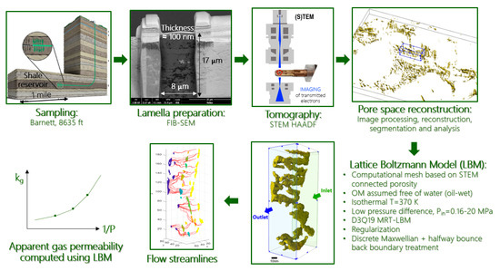
Figure 1.
Workflow from sample acquisition to preparation to STEM tomography to transport simulation.
The first stages in the workflow rely substantially upon imaging and image processing. A key early step is preparation of a roughly 100 nm thick lamella of shale, achieved by FIB-SEM ion milling. Because pore sizes in shale are on the order of nm, the imaging technique needs to have similar resolution. While FIB-SEM has been used in a number of studies for pore-space characterization [4,5,7,13], Scanning Transmission Electron Microscopy (STEM) provides superior spatial resolution. Because 3D realizations of pore space are needed for transport calculations, STEM tomography is used to obtain a volumetric representation of the sample pore network. STEM tomography is conceptually similar to X-ray CT techniques and amenable to pore space reconstruction and statistical analysis of the pore size, shape, and frequency. The pore network is processed to remove unconnected pores that do not contribute to transport but would result in longer computational times. LBM simulations incorporating a combined half-way bounce-back and discrete Maxwellian diffusion boundary treatment in three dimensions are used to simulate gas flow in the shale sample [20]. Apparent gas permeability is calculated based on Darcy’s law using simulation results including Klinkenberg-type effects.
While sample preparation and imaging are time consuming (multiple days), we believe that such characterization via digital rock physics is overall time efficient. Thus, it is a complement to conventional petrophysical measurements. Moreover, once the pore space images are obtained, they are amenable to a number of simulation types in addition to LBM, such as molecular dynamics.
3. STEM Tomographic Imaging
A clay-rich, siliceous, and mature shale sample from the Barnett formation (8635 ft) was selected for this study. The Barnett is one of the most prolific shale plays and is of intense interest. The sample was characterized using X-ray diffraction as containing substantial clay and organic matter (26 wt% illite; 10 wt% mixed illite/smectite; 13 wt% TOC) as well as siliceous material (42 wt% quartz; 4.1 wt% feldspar), while remaining very carbonate poor.
A subsample was cut parallel to bedding, was polished, and was mounted for electron microscopy. STEM is based on the transmission of a beam of electrons through relatively thin samples. Roughly 100 nm thick sections of material (i.e., lamellae) were needed to produce volumetric projections with nanometer resolution. Shale lamella preparation was achieved by FIB-SEM serial cross-sectioning and imaging. A FEI Helios Nanolab 600i was used to mill into samples with nm precision, with a gallium ion (Ga+) Focused Ion Beam (FIB) (ion milling voltage: 5–30 kV). These settings did not cause excessive heating or damage to the shale sample. A trench was milled on each side of the rectangular material that became a lamella. A U-shaped cut was then made to free the sample. Cross-sections were extracted by an omniprobe micromanipulator needle, mounted on a TEM grid, and thinned down to electron transparency. While milling, Scanning Electron (SE) imaging was used for monitoring and imaging.
The STEM High-Angle Annular Dark-Field (HAADF) imaging mode was found to highlight composition with suitable contrast, and was therefore preferred for mineral segmentation of heterogeneous shales. We acquired STEM tomograms at high magnification of regions of interest inside the lamella. The tilt series were collected by rotating the thin section to ±60° from the horizontal. Each image in the tilt series was focused manually because autofocus was not sufficient.
The volumetric sampling at each angle was 2.5 µm × 2.5 µm × 100 nm and the individual voxel resolution was 1.24 × 1.24 × 1.5 nm. Alignment, image processing, 3D reconstruction and segmentation were needed to extract quantitative information from image datasets. Stage shifts and tilt series misalignments were corrected using Inspect3D (Version 3.0, ThermoFisher Scientific, Waltham, MA, USA). A stack of parallel slices was then reconstructed by Weighted Back Projection (WBP) using TomoJ (Version 2.6, plug-in for ImageJ, public domain). The image stack was then segmented on the machine learning-based pixel classification software Ilastik (Version 1.3.3, open source), in order to extract the pore network volume. Visualization and pore scale analysis were performed using Avizo (Version 9.7.0, ThermoFisher Scientific, Waltham, MA, USA), with the methodology described in Frouté and Kovscek [15]. In anticipation of flow simulations using LBM, each two-dimensional image is converted to a binary matrix with ones and zeros representing pore and solid phases, respectively. The computation domain is constructed by stacking these binary matrices.
4. Lattice Boltzmann Method
Due to the dominance of nm-sized pore structures, flows occurring in the shale matrix mainly fall within slip flow or transitional flow regimes where the continuum assumption may not be valid. LBM is suitable for simulating flow in mesoscopic systems [20,22,23] and is used to investigate the transport of methane in a complex nano-scale pore network.
4.1. Governing Equations
The lattice Boltzmann method solves the lattice Boltzmann equation given by [24]
where is the index of the discrete velocity, is the particle distribution function at position and time . We employ the three-dimensional, nineteen-velocity (D3Q19) model where each node delivers particles in a total of nineteen directions as shown in Figure 2. These nineteen directions comprise the node itself (the zero vector), six towards the centroid of each face of the cube (Figure 2), and the remaining twelve are directed towards the midpoint of each edge. The multiple relaxation time (MRT) collision operator is used, as [25]
where is a transformation matrix projecting the distribution functions onto a momentum space. is the diagonal collision matrix given by
where denotes relaxation time and the subscripts refer to the moment: are related to conserved quantities, mass and momentum. and are related to non-conserved moments (i.e., internal energy, internal energy square, energy flux and stress tensor, respectively). Finally, and are related to the cubic and fourth-order polynomials of the momentum. The MRT collision operator enables relaxation of each momentum in accordance with the corresponding physical process. In particular, and [26]. is related to slip velocity and is discussed later. is related to fluid viscosity and is given by [27,28]
where is the lattice number along the characteristic length and is given by The particle distribution function at equilibrium is [29]
where is the square lattice speed of sound given by . The lattice weights, , are given by , , and . The macroscopic fluid density and velocity are calculated as
and
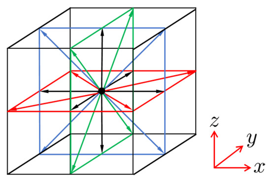
Figure 2.
Schematic of a D3Q19 LBM model.
4.2. Regularization
The discretization scheme is equivalent to projection of the particle distribution function onto a subspace spanned by the leading Hermite orthonormal basis, denoted by [30,31]. The equilibrium distribution function, , is properly projected onto because it maintains second-order terms in its Hermite expansion. However, may not be projected onto due to higher order terms. Therefore, a regularization procedure is used to address this shortcoming [31,32]. The distribution function is expressed as
where is the non-equilibrium component of the distribution. The projection of onto the second-order Hermite expansion is given by
where is the second-order Hermite polynomial, given by
where is the Kronecker delta. Replacing with and substitution of Equations (2) and (8) into (1) yields
4.3. Boundary Conditions
Constant pressure conditions are imposed at the inlet and outlet faces [33,34]. On solid boundaries, we extend the boundary treatment proposed by Wang and Aryana [20] to three dimensions to capture the slip velocity. The second order slip boundary condition is expressed as
where and are the slip coefficients, is the wall normal vector, and the subscript denotes a quantity at the wall. A combination of the discrete Maxwellian and half-way bounce-back boundary condition was used, given by
where is the portion of discrete Maxwellian part in the combination, is the distribution function calculated by discrete Maxwellian diffusion, and is the distribution function calculated by the half-way bounce-back scheme. The value of is given by
where [20]. The bounce-back scheme is
where is the distribution function in the opposite direction to . The Maxwellian diffusion, , is calculated as
where
In Equation (17), , where is the unit normal vector to the boundary, and is the wall velocity. The parameter in Equation (3) is given by
with [20].
4.4. Local Knudsen Number
As shown in Equation (4), is dependent on local and , that are related to local characteristic lengths. For the nodes on the medial axis, is evaluated by doubling the distance between the node and the boundary. For all other nodes, is equal to their distance from the nearest medial axis node.
5. Results
The LBM implementation described above is verified by comparing results with solutions form the Linearized Boltzmann Equation (LBE) and Discrete Simulation Monte Carlo (DSMC) from the literature (see [20] for details). Our workflow from STEM imaging to LBM transport simulations to macroscopic quantities of interest is demonstrated using the clay-rich, mature Barnett shale sample.
5.1. STEM Tomography
A three-dimensional reconstruction by STEM tomography of the Barnett lamella finds the following volume fractions: mineral matrix (87.8%), organic matter (11%) and porosity (1.2%). A representation of the extracted pore network shows that pores down to a few nanometers are well resolved and that nm-sized flow pathways exist across the thin section. In shale systems, pores are commonly associated with organic matter, the clay-rich mineral matrix, or cracks and fractures. Organic pores typically dominate in number and make important contributions to the storage capacity and transport properties as they trap adsorbed gas and free gas. An analysis of the pore space shows that the STEM-based porosity is entirely associated with the organic phase. The surrounding organic matter displays a spongy texture, consistent with gas-window thermal maturity. Additional pore-space analysis of this sample by FIB-SEM imaging and STEM tomography is given in Frouté and Kovscek [15].
Within the reconstructed lamella, we select a sub-volume to create a computational mesh suitable for simulation. The following selection criteria were applied: (1) the sub-volume occupies a central position close to eucentric height on the lamella, therefore remaining in objective focus during tomography and providing the most accurate 3D reconstruction, (2) the sub-volume is located in a region with excellent STEM contrast, therefore limiting pore voxel misclassification during segmentation, (3) the sub-volume comprises no more than 1 million cells, (4) the sub-volume is located in an area of relatively large porosity and pore connectivity suitable for transport simulation. The resulting sub-volume comprises roughly 1 million voxels (voxel size: 1.24 × 1.24 × 1.5 nm). We extract the porosity that is connected across the x-dimension (Figure 3a).

Figure 3.
Visualization of the porosity extracted from the STEM reconstruction (pixel size: 1.24 × 1.24 × 1.5 nm). Note: in this representation, we look upon the outlet face used for simulations. (a) Extracted pore volume connected across the x-dimension (6.5% porosity); (b) The 4 existing flow pathways. (c) Individual pores.
Flow through the lamella occurs primarily along pore channels with dimensions on the order of tens of nanometers. Smaller pores of a few nanometers do not form percolating pathways across the x-dimension and are not shown in this representation. Figure 3b shows the four pathways where flow occurs through the lamella. According to the nomenclature present in the literature [4,9], pores in this sub-volume are classified as intra-organic (pores hosted within the organic matter) and inter-organic (pores at the interface between organic matter and minerals). These organic pores are induced by the thermal maturation of kerogen and create oil-wet flow paths for hydrocarbons through the organic phase. The nature of the pore space (i.e., an oil-wet, hydrocarbon-filled system of interconnected organic pores permeating through the organic phase) therefore provides a representative image-based computational domain to simulate hydrocarbon transport. We expect LBM simulations to offer an insight into methane flow through the distinct organic nanopore channels.
We now subdivide the pore volume into individual pores (Figure 3c). The reconstructed pores display an elongated tubular shape, some tortuosity, and a strong anisotropy. In shale systems, interstitial patches of organic matter often align with bedding planes and with the geometry and orientation of enclosing minerals. It is therefore common for organic pores themselves to align with the surrounding mineral geometry. Work by Minler et al. suggests that the size and shape of organic pores depend on the kerogen content and the geometry of enclosing minerals [12]. Multiple imaging studies also report examples of intra-organic porosity being anisotropic and bearing elongated, eccentric shapes, as well as inter-organic porosity resembling curved lamellae conforming to the shape and orientation of neighboring minerals [9,11]. The preferred orientation and elongated structure of the organic nanoporosity reported in this work is therefore consistent with other examples of shale microstructures imaged at nanometer resolution [9,11,12].
The equivalent diameter, defined as the diameter of a sphere of the same volume, is often used to describe nanopores. Given that most of the reconstructed pores are not spherical and have tubular geometries, we used Feret diameters to provide a better representation of shape attributes. The Feret diameter is a one-dimensional measurement that estimates the dimension of an object in a given direction. For tubular pores, we assume that the maximum of the Feret diameters is a good representation of pore length. The minimum of the Feret diameters is a good representation of pore width. The distribution of pore widths and lengths is shown in Figure 4. Pore dimensions are on the order of tens of nanometers, with the distribution of pore widths centered around 20 nm, and pore lengths up to roughly 100 nm.

Figure 4.
Pore size distribution (pore width and length are measured with Feret diameters).
5.2. Construction of the Computational Mesh
Each image in the reconstructed tomographic stack is binarized, with ones and zeros representing pore and solid phases, respectively. The resulting images are combined to create a 3D computational domain of cells (length width height). The remaining disconnected pores are removed from the computational domain to improve computational efficiency. These pores are identified by their constant pressure, which remains equal to the initial pressure condition in a preliminary simulation run.
5.3. LBM Gas Flow Simulations
We calculate the permeability of the sample by simulating gas flow in the shale matrix using LBM as described above. A constant pressure condition is applied at the inlet and outlet faces. We consider four cases with the reference Knudsen number, , defined as the ratio of the molecular mean free path over the mean value of characteristic length, given by 0.045, 0.223, 1.117, and 5.583. The distribution of the characteristic length in the domain is presented in Figure 5 with a mean of 6.5 nm.
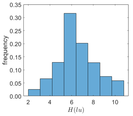
Figure 5.
Distribution of local characteristic length in lattice units.
Figure 6 shows the distribution of density and flow streamlines inside the sample in the case of . In the LBM framework, pressure is related to density in a linear fashion given by . As such, Figure 6 shows density differences, as a surrogate for pressure distribution, that develop in the domain once the steady state flow condition is reached. The maximum density in Figure 6 is 5 lattice units corresponding to 20 MPa. The maximum density difference in the domain is lattice units corresponding to 2 Pa. Streamlines show the tortuous pathways that connect the inlet to the outlet. Figure 7 compares normalized velocity maps of two slices at (Figure 7a,c) and (Figure 7b,d). As highlighted by boxes in Figure 7, compared to the case of , variations of normalized velocity across pores are less significant in the case of . This indicates that the relative magnitude of slip velocity, defined as the ratio of velocity near the wall over that in the middle of the flow pathway, is larger at a greater number.

Figure 6.
Distribution of density in lattice units and streamlines at steady state in the shale sample at .

Figure 7.
Normalized velocity maps at steady state. (a) at ; (b) at ; (c) at ; and (d) at .
The apparent gas permeability is calculated as [22,23]:
where is dynamic viscosity of gas, is the length of the domain in the mean flow direction, is the average velocity at the outlet, and and are the inlet and outlet pressures, respectively. As seen in Figure 8 where results are plotted against the reciprocal mean pressure, , apparent gas permeability increases as the mean pressure decreases; apparent permeability may be described using a quadratic polynomial in reciprocal mean pressure [20]. A smaller mean pressure leads to a larger number and an enhanced flow. This is consistent with observations shown in Figure 7.

Figure 8.
Apparent gas permeability of the shale sample versus inverse pressure.
6. Discussion
Importantly, sufficient numerical tools exist to estimate the permeability of nanoporous media given proper imaging of nanoporosity and the differentiation of connected and unconnected porosity. The use of electron microscopy techniques for direct pore-scale investigation has become common practice recently and succeeds in addressing issues of resolution, particularly for heterogeneous porous media with nm-sized pores such as shale. STEM microscopes have emerged as powerful tools uniquely capable of probing nanometric pore features in 2D and 3D. Thereby, they aid greatly in making sense of the contribution of nanoporosity towards macroscopic petrophysical attributes.
Despite state-of-the-art imaging capabilities, STEM tomography has a few limitations. High-resolution invariably limits the field of view studied, particularly in the depth of the sample. This makes the extraction of representative networks challenging and increases the need for upscaling. Additionally, ion and electron beams may cause excessive heating or damage to the shale sample rendering changes to the shale fabric. This can often be avoided by lowering the electron beam current or using cryogenic electron microscopy methods [35,36,37]. Because electron microscopes operate under vacuum, they also prevent measurements with pore pressures and overburden conditions that would be truly representative of reservoir conditions. In this study, we strive to maintain the integrity of the sample with low-voltage beam settings, to reconstruct the nanoporous network as reliably as possible from high-quality images, and to apply a rigorous image processing and reconstruction workflow. We capture volumetric representations of pore networks associated with the organic phase forming flow paths of a few tens of nanometer in width across the shale sample.
A sensitivity study conducted by measuring pixel misclassifications over repeated segmentations shows little uncertainty in the resulting porosity and pore structure [15]. Despite its relatively large porosity (6.5%), the sub-volume selected for simulation is representative of the geometry of the connected pathways found across the lamella, with pore dimensions on the order of tens of nanometers. Given the volumetric sampling and voxel size, we estimate that STEM observations are representative of pore widths between 5 and 50 nm. The lower resolution limit (about 5 nm) and the constraint on the size of the computational volume (1 million cells) are limitations to be explored in future work.
The validity of pore-scale simulations based on digital rock reconstructions is conditioned by the pertinence of the imaging scale chosen and of the physics included in the simulation. The nature of the pore space extracted by STEM tomography (i.e., an oil-wet network of interconnected organic pores permeating through the organic phase) provides a representative system to simulate hydrocarbon transport. The complex pore network is dominated by pore channels of tens of nanometer in diameter that represent a valid volumetric domain for the study of methane transport in slip flow and transitional flow regimes. Our study uniquely integrates fine-scale 3D STEM tomographic imaging, pore-space reconstruction, and numerical simulation tools using the LBM method to describe gas flow in slip, transitional, and Knudsen diffusion regimes.
In the simulation of the transport of methane, we utilize a combined Maxwellian diffusive reflection and half-way bounce-back to recover the second-order slip boundary condition. This boundary treatment is developed to deal with complex geometries due to its efficient local computation of distribution functions at nodes near boundaries. Moreover, this scheme captures slip velocities in slip flow and transitional flow regimes that dominate gas transport in unconventional reservoirs. Simulation results suggest that the apparent gas permeability depends on the mean pressure of the sample in a nonlinear fashion. This observation may help develop reliable formulations for matrix permeability in shale systems at the field-scale.
For gas flow at relatively large numbers, the confined environment may lead to remarkable interactions between molecules and walls. As a result, the thermodynamic properties of gas deviate from that at bulk condition. Moreover, the fluid density exhibits non-uniform distribution: density near the wall is greater than that in the middle of the flow channel [38,39,40]. This adsorption effect may make a substantial contribution to the overall transport in pores in the organic matrix. In the future, the LBM model shall be extended by accounting for interactions between molecules, and between molecules and boundaries under nanoconfinement. The model framework will also be extended to larger computational volumes by taking advantage of parallelized LBM calculations. Larger domains allow for the incorporation of greater details of heterogeneity of pore size, shape, and mineral composition important to upscaling efforts.
7. Conclusions
We demonstrated a digital rock workflow combining 3D Scanning Transmission Electron Microscopy (STEM) tomography with numerical simulation methods to study methane transport through the nanoporous matrix of shale with permeability in the range of tens of nD. The workflow proceeds from sample preparation, to image acquisition by STEM tomography, to volumetric reconstruction to pore-space discretization to numerical simulation of pore-scale transport. STEM tomography images offer unprecedented insights into the structure and geometry of complex nano-scale porosity within a Barnett shale thin section. LBM provides a tool to transform spatial data into information relevant to transport of gases and liquids. We selected a sub-volume to create a computational mesh suitable for simulation, comprised of roughly 1 million voxels (sub-volume: 79 × 82 × 194 nm, voxel size: 1.24 × 1.24 × 1.5 nm). Elongated pore channels with dimensions on the order of tens of nanometers form connected pathways across the organic phase. LBM simulations offer an insight into the pressure distribution and velocity profiles through the distinct pore channels. Using LBM, an apparent gas permeability in the range of 10−19 to 10−16 m2 (0.1 to 100 µD) is computed for the selected sub-volume. All in all, the workflow incorporating three-dimensional measurements on the nm scale with numerical simulations of flow through the pore network images provides further insight into fluid transport within shale. Importantly, the workflow is extendable to larger images and a larger range of pore spaces.
Author Contributions
Conceptualization, L.F., Y.W., J.M., A.R.K., S.A.A.; methodology, L.F., Y.W., A.R.K., S.A.A.; software, Y.W., J.M.; investigation, L.F., Y.W., J.M.; data curation, L.F., Y.W.; writing—original draft preparation, L.F., Y.W., J.M.; writing—review and editing, A.R.K., S.A.A.; supervision, A.R.K., S.A.A.; project administration, A.R.K., S.A.A.; funding acquisition, A.R.K., S.A.A. All authors have read and agreed to the published version of the manuscript.
Funding
This work was supported as part of the Center for Mechanistic Control of Water-Hydrocarbon-Rock Interactions in Unconventional and Tight Oil Formations (CMC-UF), an Energy Frontier Research Center funded by the U.S. Department of Energy (DOE), Office of Science, Basic Energy Sciences (BES), under Award # DE-SC0019165. L.F. acknowledges TOTAL S.A. for a graduate fellowship.
Acknowledgments
Experimental results were obtained at the Stanford Nano Shared Facilities (SNSF), supported by the National Science Foundation under award ECCS-2026822.
Conflicts of Interest
The authors declare no conflict of interest. The funders had no role in the design of the study; in the collection, analyses, or interpretation of data; in the writing of the manuscript, or in the decision to publish the results.
References
- Blunt, M.J.; Bijeljic, B.; Dong, H.; Gharbi, O.; Iglauer, S.; Mostaghimi, P.; Paluszny, A.; Pentland, C. Pore-scale imaging and modelling. Adv. Water Res. 2013, 51, 197–216. [Google Scholar] [CrossRef]
- Blunt, M.J. Multiphase Flow in Permeable Media: A Pore-Scale Perspective; Cambridge University Press: Cambridge, UK, 2017. [Google Scholar]
- Guan, K.M.; Nazarova, M.; Guo, B.; Tchelepi, H.A.; Kovscek, A.R.; Creux, P. Effects of image resolution on sandstone porosity and permeability as obtained from X-ray microscopy. Transp. Porous Media 2019, 127, 233–245. [Google Scholar] [CrossRef]
- Loucks, R.G.; Reed, R.M.; Ruppel, S.C.; Hammes, U. Spectrum of pore types and networks in mudrocks and a descriptive classification for matrix-related mudrock pores. AAPG Bull. 2012, 96, 1071–1098. [Google Scholar] [CrossRef]
- Bernard, S.; Brown, L.; Wirth, R.; Schreiber, A.; Schulz, H.M.; Horsfield, B.; Aplin, A.C.; Mathia, E.J. FIB-SEM and TEM Investigations of an Organic-rich Shale Maturation Series form the Lower Toarcian Posidonia Shale, Germany: Nanoscale Pore System and Fluid-rock Interactions. Electron Microsc. Shale Hydrocarb. Reserv. AAPG Mem. 2013, 102, 53–66. [Google Scholar] [CrossRef]
- Chen, L.; Kang, Q.; Pawar, R.; He, Y.; Tao, W. Pore-scale prediction of transport properties in reconstructed nanostructures of organic matter in shales. Fuel 2015, 158, 650–658. [Google Scholar] [CrossRef]
- Zhou, S.; Yan, G.; Xue, H.; Guo, W.; Li, X. 2D and 3D nanopore characterization of gas shale in Longmaxi formation based on FIB-SEM. Mar. Pet. Geol. 2016, 73, 174–180. [Google Scholar] [CrossRef]
- Berthonneau, J.; Obliger, A.; Valdenaire, P.L.; Grauby, O.; Ferry, D.; Chaudanson, D.; Levitz, P.; Kim, J.J.; Ulm, F.J.; Pellenq, R.J.M. Mesoscale structure, mechanics, and transport properties of source rocks’ organic pore networks. Proc. Natl. Acad. Sci. USA 2018, 115, 12365–12370. [Google Scholar] [CrossRef]
- Ma, L.; Slater, T.; Dowey, P.J.; Yue, S.; Rutter, E.H.; Taylor, K.G.; Lee, P.D. Hierarchical integration of porosity in shales. Sci. Rep. 2018, 8, 11683. [Google Scholar] [CrossRef] [PubMed]
- Goral, J.; Walton, I.; Andrew, M.; Deo, M. Pore system characterization of organic-rich shales using nanoscale-resolution 3D imaging. Fuel 2019, 258, 116049. [Google Scholar] [CrossRef]
- Wu, T.; Zhao, J.; Zhang, W.; Zhang, D. Nanopore structure and nanomechanical properties of organic-rich terrestrial shale: An insight into technical issues for hydrocarbon production. Nano Energy 2020, 69, 104426. [Google Scholar] [CrossRef]
- Milner, M.; McLin, R.; Petriello, J. Imaging Texture and Porosity in Mudstones and Shales: Comparison of Secondary and Ion-Milled Backscatter SEM Methods. In Proceedings of the SPE/AAPG/SEG Unconventional Resources Technology Conference, Austin, TX, USA, 20–22 July 2010. [Google Scholar] [CrossRef]
- Anderson, T.I.; Vega, B.; Kovscek, A.R. Multimodal imaging and machine learning to enhance microscope images of shale. Comput. Geosci. 2020, 145, 104593. [Google Scholar] [CrossRef]
- Kim, T.W.; Ross, C.M.; Guan, K.M.; Burnham, A.K.; Kovscek, A.R. Permeability and Porosity Evolution of Organic-Rich Shales from the Green River Formation as a Result of Maturation. In Proceedings of the Canadian Unconventional Resources and International Petroleum Conference, Calgary, AB, Canada, 19–21 October 2020; Volume 25, pp. 1377–1405. [Google Scholar] [CrossRef]
- Frouté, L.; Kovscek, A.R. Nano-Imaging of Shale Using Electron Microscopy Techniques. In Proceedings of the SPE/AAPG/SEG Unconventional Resources Technology Conference, Austin, TX, USA, 20–22 July 2020; p. 3283. [Google Scholar] [CrossRef]
- Soulaine, C.; Tchelepi, H.A. Micro-continuum approach for pore-scale simulation of subsurface processes. Transp. Porous Media 2016, 113, 431–456. [Google Scholar] [CrossRef]
- Guo, B.; Ma, L.; Tchelepi, H.A. Image-based micro-continuum model for gas flow in organic-rich shale rock. Adv. Water Res. 2018, 122, 70–84. [Google Scholar] [CrossRef]
- Chen, L.; Zhang, L.; Kang, Q.; Viswanathan, H.S.; Yao, J.; Tao, W. Nanoscale simulation of shale transport properties using the lattice Boltzmann method: Permeability and diffusivity. Sci. Rep. 2015, 5, 1–8. [Google Scholar] [CrossRef]
- Wang, J.; Kang, Q.; Chen, L.; Rahman, S.S. Pore-scale lattice Boltzmann simulation of micro-gaseous flow considering surface diffusion effect. Int. J. Coal Geol. 2017, 169, 62–73. [Google Scholar] [CrossRef]
- Wang, Y.; Aryana, S.A. Pore-scale simulation of gas flow in microscopic permeable media with complex geometries. J. Nat. Gas Sci. Eng. 2020, 81, 103441. [Google Scholar] [CrossRef]
- Karniadakis, G.; Beskok, A.; Aluru, N. Microflows and Nanoflows: Fundamentals and Simulation; Springer Science & Business Media: New York, NY, USA, 2005. [Google Scholar]
- Ning, Y.; Jiang, Y.; Liu, H.; Qin, G. Numerical modeling of slippage and adsorption effects on gas transport in shale formations using the lattice Boltzmann method. J. Nat. Gas Sci. Eng. 2015, 26, 345–355. [Google Scholar] [CrossRef]
- Wang, J.; Kang, Q.; Wang, Y.; Pawar, R.; Rahman, S.S. Simulation of gas flow in micro-porous media with the regularized lattice Boltzmann method. Fuel 2017, 205, 232–246. [Google Scholar] [CrossRef]
- Chen, S.; Doolen, G.D. Lattice Boltzmann method for fluid flows. Annu. Rev. Fluid Mech. 1998, 30, 329–364. [Google Scholar] [CrossRef]
- D’Humieres, D. Multiple–relaxation–time lattice Boltzmann models in three dimensions. Philos. Trans. R. Soc. Lond. Ser. A 2002, 360, 437–451. [Google Scholar] [CrossRef]
- Suga, K. Lattice Boltzmann methods for complex micro-flows: Applicability and limitations for practical applications. Fluid Dyn. Res. 2013, 45, 034501. [Google Scholar] [CrossRef]
- Michalis, V.K.; Kalarakis, A.N.; Skouras, E.D.; Burganos, V.N. Rarefaction effects on gas viscosity in the Knudsen transition regime. Microfluid. Nanofluid. 2010, 9, 9847–9853. [Google Scholar] [CrossRef]
- Li, Q.; He, Y.L.; Tang, G.H.; Tao, W.Q. Lattice Boltzmann modeling of microchannel flows in the transition flow regime. Microfluid. Nanofluid. 2011, 10, 607–618. [Google Scholar] [CrossRef]
- Chen, H.; Chen, S.; Matthaeus, W.H. Recovery of the Navier-Stokes equations using a lattice-gas Boltzmann method. Phys. Rev. A 1992, 45, R5339. [Google Scholar] [CrossRef] [PubMed]
- Zhang, R.; Shan, X.; Chen, H. Efficient kinetic method for fluid simulation beyond the Navier-Stokes equation. Phys. Rev. E 2006, 74, 046703. [Google Scholar] [CrossRef] [PubMed]
- Shan, X.; Yuan, X.F.; Chen, H. Kinetic theory representation of hydrodynamics: A way beyond the Navier–Stokes equation. J. Fluid Mech. 2006, 550, 413–441. [Google Scholar] [CrossRef]
- Latt, J.; Chopard, B. Lattice Boltzmann method with regularized pre-collision distribution functions. Math. Comput. Simul. 2006, 72, 165–168. [Google Scholar] [CrossRef]
- Zou, Q.; He, X. On pressure and velocity boundary conditions for the lattice Boltzmann BGK model. Phys. Fluids 1997, 9, 1591–1598. [Google Scholar] [CrossRef]
- Hecht, M.; Harting, J. Implementation of on-site velocity boundary conditions for D3Q19 lattice Boltzmann simulations. J. Stat. Mech. Theory Exp. 2010, 2010, P01018. [Google Scholar] [CrossRef]
- Deglint, H.J.; Clarkson, C.R.; DeBuhr, C.; Ghanizadeh, A. Live imaging of Micro-Wettability experiments performed for Low-Permeability oil Reservoirs. Sci. Rep. 2017, 7, 1–13. [Google Scholar] [CrossRef]
- Lubelli, B.; de Winter, D.A.M.; Post, J.A.; van Hees, R.P.J.; Drury, M.R. Cryo-FIB-SEM and MIP study of porosity and pore size distribution of bentonite and kaolin at different moisture contents. Appl. Clay Sci. 2013, 80–81, 358–365. [Google Scholar] [CrossRef]
- Schmatz, J.; Urai, J.L.; Berg, S.; Ott, H. Nanoscale imaging of pore-scale fluid-fluid-solid contacts in sandstone. Geophys. Res. Lett. 2015, 42, 2189–2195. [Google Scholar] [CrossRef]
- Wang, Y.; Aryana, S.A. Coupled confined phase behavior and transport of methane in slit nanopores. Chem. Eng. J. 2020, 404, 126502. [Google Scholar] [CrossRef]
- Yu, H.; Chen, J.; Zhu, Y.; Wang, F.; Wu, H. Multiscale transport mechanism of shale gas in micro/nano-pores. Int. J. Heat Mass Transf. 2018, 111, 1172–1180. [Google Scholar] [CrossRef]
- Zhao, J.; Yao, J.; Zhang, L.; Sui, H.; Zhang, M. Pore-scale simulation of shale gas production considering the adsorption effect. Int. J. Heat Mass Transf. 2016, 103, 1098–1107. [Google Scholar] [CrossRef]
Publisher’s Note: MDPI stays neutral with regard to jurisdictional claims in published maps and institutional affiliations. |
© 2020 by the authors. Licensee MDPI, Basel, Switzerland. This article is an open access article distributed under the terms and conditions of the Creative Commons Attribution (CC BY) license (http://creativecommons.org/licenses/by/4.0/).