Article

Modeling of Axial Flux Permanent Magnet Generators

by
Natalia Radwan-Pragłowska
,
Tomasz Węgiel
* and
Dariusz Borkowski
Faculty of Electrical and Computer Engineering, Cracow University of Technology, Warszawska 24 St., 31-155 Cracow, Poland
*
Author to whom correspondence should be addressed.
Energies 2020, 13(21), 5741; https://doi.org/10.3390/en13215741
Submission received: 28 August 2020 / Revised: 14 October 2020 / Accepted: 29 October 2020 / Published: 2 November 2020
(This article belongs to the Special Issue Permanent Magnet Electrical Machines)

Abstract

:
This article focuses on modeling of an Axial Flux Permanent Magnet Generator (AFPMG). The authors analyzed selected variants of disk generators, including coreless stator constructions and with iron core ones, also taking into account the Permanent Magnet (PM) arrangement in order to show the way to obtain the optimal machine characteristics based on analytical equations. In addition to the full model, which takes into account the higher harmonics of the magnetic field distribution, the paper presents a simplified mathematical model developed for generator operation cases such as standalone, connected to a 3-phase power grid and loaded with a diode rectifier. The analytical and finite-element method (FEM) calculations were performed as well as laboratory tests to confirm the correctness of presented model assumptions.

1. Introduction

The interest in synchronous generators excited by Permanent Magnets (PM) is related to the global tendencies to support the power industry with the help of local power plants based on renewable energy sources such as water or wind energy, in which PM synchronous generators are often used. For these solutions, it is possible to develop a structure with a very large pole number and relatively small dimensions. The aim of the work is related to the search for design solutions for electromechanical energy converters with permanent magnets dedicated to small power plants. These include machines excited by PM with a radial magnetic field as well as disk machines with an axial flux permanent magnetic field [1,2,3,4,5,6,7].
The first Axial Flux Permanent Magnets (AFPM) machines appeared in the 1830s [8]. In 1831 M. Faraday constructed a unipolar generator (the so-called Faraday disk), which was a machine with axial magnetization. This type of machine also appeared in N. Tesla’s patent [9], published in 1889. Earlier, in 1837, there was also a patent by T. Davenport [8], in which the first machine with axial magnetization was described. However, the wider development of axially magnetized machines started after 1983, when modern high-energy rare earth permanent magnets based on the combination of Neodymium, Iron and Boron appeared.
Currently produced AFPM machines are characterized by a simple design and relatively small dimensions, especially in the rotor axis, as well high torque-to-weight ratio and efficiency. These benefits sometimes give AFPM machines advantages over conventional machines. AFPM machines are commonly used in various applications. In papers from the recent years, apart from the structural analyses of AFPM generators used for wind farms [1,3,4,5], there are more and more other possibilities of their use. One can mention here electric cars, traction drives and low-speed vehicles [2,7,8,10].
The stator construction of AFPM machines can be with or without armature slots, with or without armature core [8,10]. Among the commonly used stator designs, there are two variants of the stator coil arrangement: non-overlapping and overlapping windings [11,12]. The structure of the rotor is based on the selection of its type: internal or external permanent-magnet rotors, with surface-mounted or interior permanent-magnet and as single-stage or multistage [8].
In recent years, a lot of research has been carried out to optimize the design and modelling of AFPM machines [13,14,15,16,17,18,19,20,21,22,23,24,25,26,27,28]. There are considerations for which analyses are carried out strictly on the basis of calculations of the magnetic field distribution with the use of numerical methods based on the finite-element method (FEM) [18,21,24] and with the use of analytical models which also allow one to obtain quantitatively satisfactory results. However, numerical modeling techniques do not easily allow a synthesized study for phenomena occurring in the machine, hence analytical models are very popular. For AFPM machines, there are some areas for which one can make some interesting considerations regarding complementation of the analytical models, similar to classic aspects of electrical machine modelling. Basically, analytical models are based on two approaches, analytical resolutions of the Maxwell’s equations [13,14,15,17,19,20,23] and the magnetomotive force (MMF) by the permeance product [16,22,25,26,27,28]. The first analytical approach leads to very complex equations that are often difficult to accept by engineers. Mathematical models based on permeance functions are more understandable for designers. Additionally, these models allow for analyzing the formation and reduction of cogging torques for iron core AFPM machines [25,26,27,28].
The aim of this article is the presentation of a universal analytical methodology that allows for comprehensive modelling of various designs of AFPM machines. This approach has not been widely published for this class of machines. This paper focuses in particular on a representative case of AFPM disc generators with a stationary stator with non-overlapping windings and two rotor discs. These solutions are well known; however, the aim of this work is to modify the structure and consequently, to correct the analytical mathematical models. The mentioned structure was chosen because of its simplicity, with the possibility of modifying the stator (coreless; with cores) and the arrangement of the permanent magnets (simple; skewed), in order to improve the generator characteristics and parameters, in particular to increase the obtained power and reduce the cogging torque. In this article, the four structures of AFPM generators ware considered, taking into account the higher harmonics of flux density distributions. An additional aspect of created models is their usability for operational purposes, e.g., cooperation with a six-pulse diode rectifier, which was also presented in this paper. The correctness of the result was obtained on the basis of the created mathematical models, and it was verified on the basis of laboratory tests and FEM calculations.

2. Mathematical Model

A generator with non-overlapping stator windings and permanent magnets placed on one side of two rotor disks was selected for the further analysis. The model created in ANSYS Maxwell software is shown in Figure 1. The generator model was divided into ten regions, with a separate mesh defined for each. The total number of tetrahedral elements (for the basic model mesh) was 857,643.
The main features of considered AFPM machine with non-overlapping windings [29,30,31,32]: number of coils per phase p s , total number of stator coils 3 p s , number of magnets per 1 rotor disc 2 p   =   4 p s , p   /   p s = 2, maximum angle of coil pitch ε max = 2 π 3 p s = 4 π 3 p .
Further analyses were carried out for four generator variants: two stator designs [30,31,32] and two ways of magnets arrangement. In case of amateur solutions, these design options are quite simple and often performed.
The authors considered stator topologies shown in Figure 2: a coreless stator and a stator with iron cores placed inside the coils. Cases of simple and skewed arrangement of PM on the rotor disks were considered.

2.1. Distribution of Magnetic Field

2.1.1. Basic Model of Flux-Density Distribution Induced by PM

First of all, as the basic one for the further considerations, only the distribution of the magnetic field from permanent magnets was used. The authors assumed a linear approximation of the demagnetization characteristics of permanent magnets B m = B r + μ 0 μ rm H m and neglected the iron saturations and magnetic voltage drops. For the discussed cases, these assumptions are justified due to the relatively large dimensions of the air gaps. Despite the assumed simplicity, the problem of analytical modelling of the magnetic field distribution becomes more complicated and relatively more difficult to describe than in the case of classic machines. Based on the principles presented in exemplary literature [8,13,15,29,33,34,35], analytical equations describing the flux-density distribution in the air gap for the base model of a coreless generator were used. The cross-section is presented in Figure 3 and Figure 4. where:
  • θ—it is the angular coordinate associated with the air-gap,
  • φ—it is the angle of the rotor position with respect to the reference frame.
Approximation of the axial component of magnetic flux-density distribution induced by the permanent magnets in the middle of the air gap (component z = 0 ) for coreless AFPM machine is presented in Figure 5 [29,30,31,32].
The distribution of magnetic flux-density in the gap induced by permanent magnets can be approximated using the Fourier series [13,15,29,30,31,32]:
B m ( θ φ , r ) = ς Q B ς PM ( r ) · e j ς ( θ φ )
where the Fourier spectrum contains harmonics of ςth order, which belong to the set Q = { 5 p , 3 p , p , p , 3 p , 5 p , } .
Fourier coefficients B ς PM ( r ) can be defined using a two-dimensional (2D) model of the magnetic field distribution according to [13,15]. The 1D models in this case are too imprecise and do not provide sufficient quantitative correspondence.

2.1.2. Distribution of Flux-Density in a Machine with Real Shapes of a Magnetic Circuit

An illustration of the methodology of deriving an analytical model of the magnetic flux density distribution in the air gap was made for the model with cores [32], presented in the coordinate system according to Figure 6. Basing on this model, any other shapes of the magnetic circuit can also be inserted.
Figure 7 shows an example of windings arrangement [8] and placement of the iron cores inside the coils.
The model of magnetic flux-density distribution in the air-gap of an AFPM generator is a function of four variables (dependent on a axial component z, location according to the stator θ, angle of the rotor position φ and radial location R i r R o ). It was assumed that the general equation describing the distribution of magnetic flux-density is simplified and is considered only for the axial component z = 0 . It means that:
B δ ( z , θ , φ , r ) = B m ( z , θ , φ , r ) = B ( z = 0 , θ , φ , r )
By applying Ampere’s circuital law for the contour marked in Figure 6 and the assuming linearity of the magnetic circuit, one can get the equations describing magnetic field distribution, well known from classical considerations:
B ( z = 0 , θ , φ , r ) = B ( θ , φ , r ) = B Θ ( θ , r ) + B PM ( θ φ , r )
where:
  • B Θ ( θ , r ) —axial component of the flux-density distribution resulting from winding currents (windings magnetomotive forces MMF),
  • B PM ( θ φ , r ) —axial component of flux-density from permanent magnets.
By assuming l m ( θ φ , r ) = l m ( θ φ , r ) μ rm and defining the unit permeance function as a magnitude proportional to the inverse of the magnetic field force lines length:
λ ( θ , φ , r ) = μ 0 l δ ( θ , r ) + l m ( θ φ , r )
Function l δ ( θ , r )   in case of the cores placed inside the stator coils, can be approximated as shown in Figure 8.
And the function l m ( θ φ , r ) can be approximated as shown in Figure 9:
By defining the winding magnetomotive force (MMF) function as:
Θ s ( θ , r ) = a s ( θ , r ) d θ θ θ + 2 π Θ s ( θ , r ) d θ 0
where a s ( θ , r ) —stator ampere-turns, the axial components of flux-density can be defined as follows:
B Θ ( θ , r ) = λ ( θ , r )   { Θ s ( θ , r ) θ θ + 2 π λ ( θ , r ) · Θ s ( θ , r )   d θ θ θ + 2 π λ ( θ , r )   d θ }
B PM ( θ , φ , r ) = λ ( θ , φ , r ) λ ref ( r )   {   B m ( θ φ , r )   θ θ + 2 π λ ( θ , φ , r )   · B m ( θ φ , r )   d θ θ θ + 2 π λ ( θ , φ , r ) d θ }
where:
  • λ ref ( r ) = λ ( 0 , 0 , r ) is the reference magnitude for the origin of the coordinate system,
  • B m ( θ φ , r )   is the flux-density distribution induced by permanent magnets for a coreless machine.
The obtained Equations (6) and (7) are modifications of the well-known classical equation describing the one-dimensional distribution of the magnetic field in the air gap [33,34]. The presence of permanent magnets in the machine magnetic circuit causes some modifications in the form of an additional component B PM ( θ , φ , r ) [29,35] described by the Equation (7).
The magnetomotive force (MMF) of a 3-phase symmetrical AFPM winding (the arrangement of the stator windings is shown in Figure 7) can be described by the following relationship [29,34,35].
Θ s ( θ , r ) = a = 1 3 Θ a ( θ , r )
The Fourier distribution of the magnetomotive (Figure 10) force for the winding “a” is presented by the following equation:
Θ a ( θ , r ) = v P Θ v a ( r ) · e j v ( θ θ a )
where the Fourier spectrum of the magnetomotive force MMF contains harmonics of vth order, belonging to the set P = { 3 p s , 2 p s , p s , p s , 2 p s , 3 p s , } .
For 3-phase winding, θ a = ( a 1 ) 2 π 3 p s , where a = 1 , 2 , 3 .
The coefficients in Equation (9) are as follows:
Θ v a ( r ) = i a 1 π W v s ( r )
where: W v s ( r ) = w s · k s | v | ( r ) | v | , k s | v | —the winding factor for vth harmonic and w s —the total number of turns of the stator winding. For concentrated coils, the winding factor [8,29,34,35] can be defined as:
k s | ν |   ( r ) = sin ( | ν | ε ( r ) 2 )   · sin ( | ν | α sc ( r ) 2 ) | ν | α sc ( r ) 2
  • ε ( r ) = a c r —an angle of coil pitch or coil span at coordinate r, a c a co + a ci 2 .
  • α sc ( r ) = a sc r —an angle of the coil side width at coordinate r.
The above equations are valid for both coreless and core stators. However, in case of coreless machines, the components of the flux-density distribution have a simpler form.

2.1.3. Flux-Density Distribution in Stator Coreless Machine

The unit permeance, in general, is a function dependent on the coordinates θ, φ and r. For the machine model with a coreless stator (Figure 11), the equations described in the previous sections are significantly simplified.
Assuming again that the relative magnetic permeability of permanent magnets is similar to the air magnetic permeability ( μ rm 1.01 1.1 ) for the case of a coreless machine, the distribution of the unit permeability function can be approximated only by the constant component:
λ 0 = μ 0 l δ + 2 l m
where: l m = l m μ rm .
The MMF component describing the field distribution, depending on the winding currents for a 3-phase AFPM machine, can be presented as [29,30,31,32]:
B Θ ( θ , r ) = λ 0 · a = 1 3 ν P Θ ν a ( r )   · e j ν ( θ θ a )
The form of a component from permanent magnets is also simplified:
B PM ( θ , φ , r ) = B m ( θ φ , r ) = ς Q B ς PM ( r ) · e j ς ( θ φ )
The coefficients of a 2D magnetic flux-density component distribution from permanent magnets (the distribution preferred for the coreless stator) in the middle of the air gap according to [13,15,29,30,31,32] are as follows:
B ς PM ( r ) = 2   B r π p ς   ·   sin ( ς · β ( r ) )   2 sinh ( ς l m r ) · cosh ( ς 2   l m + l δ   2 r ) μ rm · sinh ( ς l δ + 2   l m r )
where: β ( r ) = a m 2 r ; a m a mo + a mi 2 .

2.1.4. Flux-Density Distribution in Machine with Cores

In relation to a coreless machine, the unit permeability for a machine with iron cores is a function of the radial coordinate r and a coordinate θ associated with the stator. If we re-assume that the relative magnetic permeability of PM is close to the magnetic permeability of air ( μ rm 1.01 1.1 ) the unit permeance function is independent of the rotor position (reference system to the first winding first coil axis).
The Fourier distribution of the unit permeance function (Figure 12) can be therefore defined as (16):
λ ( θ , r ) = m M λ m ( r )   · e j m θ
where:
λ m ( r ) =   { λ min + ( λ max λ min ) 3 π p s   ε ( r ) α sc ( r ) 2   for   m = 0 ( λ max λ min ) 3 π p s m sin ( m   ε ( r ) α sc ( r ) 2 )   for   m M { 0 }
λ max = μ 0 l δ l i + 2 l m λ min = μ 0 l δ + 2 l m
m-order of the permeance harmonic belonging to the set M = { 9 p s , 6 p s , 3 p s , 0 , 3 p s , 6 p s , 9 p s , } .
Magnetic flux density distribution induced by PM for AFPMG with iron cores can be analyzed using the unit permeance function and the base flux density distribution for a coreless machine. The equation describing the distribution of the flux-density component depending on the winding currents can be simplified according to the Equation (6) by eliminating the constant component according to the following equation:
θ θ + 2 π λ ( θ , r ) · Θ a ( θ , r )   d θ = { 2 π m M   ν P λ m ( r )   Θ ν a ( r )   for   m + ν = 0 0 for   m + ν 0 θ θ + 2 π λ ( θ , r ) d θ = 2 π   λ 0
Finally, one can obtain the Equation (20) describing the flux density component, dependent on the winding currents, in the form:
B Θ ( θ , r ) = a = 1 3 m M   ν P c ( m , ν ) · λ m ( r ) · Θ ν a ( r )   ·   e j ( m + ν ) θ ·   e j ( ν θ a )
where:
c ( m , ν ) = { 0   for   m + ν = 0 1     for     m + ν 0
Similar simplifications can be assumed for the flux-density component excited by PM (7). Finally, it can write:
B PM ( θ , φ , r ) = m M   ς Q c ( m , ς )   λ m ( r ) λ ref ( r )   B ς PM ( r ) · e j ( ς + m ) θ · e j ( ς )   φ
The Fourier spectrum coefficients of the flux-density distribution excited by PM, appearing in Equation (22) can be presented for a two-dimensional (2D) field distribution model in the form [13,15,29,30,31,32]:
B ς PM ( r ) = 2   B r π p ς   sin ( ς · β ( r ) ) 2   sinh ( ς   l m r ) · cosh ( ς 2 l m + l δ l i     2 r ) μ rm · sinh ( ς   2   l m + l δ l i r )

2.2. Generator Model Equations

The usage of Lagrange’s formalism, based on the characteristics of the windings and the elements co-energy function of the entire electromechanical system, allows for a mathematical modelling of the AFPMG. Basing on [29,30,31,32,33,34,35] the equations of a permanent magnet machine with a three-phase winding, (assuming sign convention for passive component) can be defined in a standard matrix form:
[ L σ s + L ss L σ s + L ss L σ s + L ss ]   d d t [ i 1 i 2 i 3 ]   + R s ·   [ i 1 i 2 i 3 ]   + d d t [ ψ PM 1 ( φ ) ψ PM 2 ( φ ) ψ PM 3 ( φ ) ]   = [ u 1 u 2 u 3 ]
J d 2 φ d t 2 = T L + T em ( i 1 , i 2 , i 3 , φ ) + T cog ( φ ) D d φ d t
where the electromagnetic torque T em and cogging torque T cog :
T em ( i 1 , i 2 , i 3 , φ ) = [ i 1 i 2 i 3 ] · φ [ ψ PM 1 ( φ ) ψ PM 2 ( φ ) ψ PM 3 ( φ ) ]
T cog = E 0 PM ( φ ) φ
E 0 PM ( φ ) —co-energy component independent of winding currents.
The above equations are quite obvious, and their structure is very similar to the Lagrange equations for conventional electrical machines. Due to the presence of permanent magnets in the machine magnetic circuit, some adjustments should be made while determining the basic parameters in relation to classic models.
In order to describe the basic parameters of the generator mathematical model (24), the winding flux linkage was defined. The equation describing the flux ψ a ( φ ) , linked with the winding “a” can be defined as:
ψ a ( φ ) =   R i R o w s   { ε ( r ) + α sc ( r ) 2 + θ a ε ( r ) α sc ( r ) 2   + θ a     B ( θ , φ , r )   d θ }   r   d r
In order to simplify, some averaging has been made by assuming that r r s = R o + R i 2 . Then flux ψ PM a , linked with winding “a”, generated by permanent magnets in zero current state, is described by standard relation:
ψ PM a ( φ ) =   ς Q   ψ ς PMs   ·   e j ς { ( a 1 ) 4 π 3 p φ } for   a   =   1 , 2 , 3
while the generator electromotive force (EMF) for winding “a” (in zero current state) at constant speed, is determined by the relationship:
e PM a = ς = p , 3 p , 5 p   E ς ·   cos ς { Ω t ( a 1 ) 4 π 3 p } for   a = 1 , 2 , 3
where: E ς = 2 ς   Ω   ψ ς PMs .
The leakage inductances are analytically expressed as the sum of two components [8]. The first one is related to the leakage flux around the active conductors’ radial part (coil sides) and the second one depends on the leakage flux around the end windings (top and bottom of the coil). The leakage inductance coefficient can be determined from following equation:
L σ s 2 μ 0 ·   ( w s ) 2   [ l c + ( a c a sc ) ]   · 0.3 / p s
where l c is the length of the active side of the coil and in most cases l c R o R i .

2.2.1. Model of Coreless Generator with Simple Magnets

The distribution function coefficients of the flux from permanent magnets linked with the stator winding (29) must be modified due to the weakening of the flux at the magnets’ edges. This correction is important for the quantitative analysis due to the relatively large air gap in the analyzed structure of discussed generator with a coreless stator.
Considering a two-dimensional distribution of flux-density in the air gap (taking into account the Equation (15)) it is possible to model the effects on the magnets side edges along the coordinate θ . A separate problem is to include the weakening of the permanent magnets flux at the edges that are perpendicular to the coordinate r (Figure 13), that is, on the inside (for r = R i ) and outer (for r = R o ) magnets edges. The proposed analytical equations allowing us to derive appropriate correction functions are not quite as complex [13,15]. In this paper, a simpler approach is proposed. Approximate distribution of the magnetic flux-density produced by PM in the middle of the air gap ( z = 0 ), along the radial coordinate, is shown in Figure 13.
The authors proposed to introduction a correction factor k e , which represents the flux weakening at the inner and outer magnets edges. This coefficient can be determined as the ratio:
k e =   B r   ( AV ) B θ   ( AV )
where:
  • B r   ( AV ) —the average value of the axial component of the magnetic flux-density distribution from PM in the middle of the air gap B m ( ( θ φ ) = 0 , r ) along the coordinate r (Figure 13) in the range of ( R i , R o ),
  • B θ   ( AV ) —the average value of the axial component of the magnetic flux-density distribution from PM in the middle of the air gap B m ( θ φ , r s ) (Equation (1), Figure 5) according to the coordinates θ φ in the range of ( β ( r s ) ,   β ( r s ) ) ,
  • B max —maximum flux-density value,
  • B edge —the value of the magnetic flux-density at the edge of the magnets.
B edge ,   B max values (Figure 13) can be determined both by finite element analysis and by using analytical equations. Using the analytical waveform approximation (Figure 13) for the cases where l c > ( l m + l δ ) one can get:
B r   ( AV )   = B max l c   ( l m + l δ ) l c + B edge l m + l δ l c + ( B max B edge ) 2 π l m + l δ l c
where:
B max = ς Q B ς PM ( r s )
l c = R o R i is the magnet length.
In case of analytical considerations, assuming that l c > ( l m + l δ ) and considering:
B edge = 1 2 B max
the Equation (33) is reduced to a very simple form:
B r   ( AV )   = B max · [   1 ( 1 2 π ) l m + l δ 2   l c ]
Basing on the analytical equations of magnetic flux-density distribution induced by PM in the middle of the air gap (1), it is possible to determine the average value of this function in the range ( β ( r s ) , β ( r s ) ) :
B θ   ( AV ) = ς Q B ς PM ( r s )   · sin   ς   β ( r s ) ς   β ( r s )
The corrected form of coefficients of flux linkages induced by PM (29) is presented by the following equation:
ψ ς PMs =   2   k e · B ς   PM ( r s )   · W ς s ( r s )   · r s · l c
After formal mathematical operations, the windings inductances can be described using standard relationships [8,34,35]:
L ss = ν P L ν ss L ν ss = 2 π   · [ W ν s   ( r s ) ] 2   · r s · l c · λ 0
Co-energy function for a coreless machine in a zero current state is constant ( E 0 PM ( φ ) = const ) and therefore the cogging torque does not occur ( T cog ( φ ) = 0 ).

2.2.2. Model of a Generator with Stator Cores and Simple Magnets

While deriving the flux linkage distribution coefficients (29), for the generator model with cores, it can be assumed that the problem of the magnet flux weakening at the inner and outer magnets edges is not so significant and there is no need to take these effects into account ( k e = 1). After formal mathematical transformations, the coefficients of the flux linkage function distribution take the following form:
ψ ς PMs = m M   2   c ( m , ς )   λ m ( r s ) λ ref ( r s )   · B ς   PM ( r s )   · W ς + m s ( r s )   · r s · l c
The windings inductances can be defined as follows [29,30,31,32,34,35]:
L ss = m M   ν P 2 π   c ( m , ν )   · W ν s   ( r s )   · W ν + m s   ( r s )   · r s · l c · λ m ( r s )
For the machine with cores, the co-energy component, independent of the winding currents, should be analyzed. This component is related to the energy stored in the air gap and in permanent magnets [35,36]. The following analysis is based on the magnetic flux-density distribution equations in the zero-current state for the base model and the unit permeance function. The co-energy component in zero current state can be defined as [35,36]:
E 0 PM ( φ ) = R i R o { 0 2 π [ B PM ( θ , φ , r ) ] 2 λ ( θ , r )   d θ }   r   d r l c   r s 2   λ ref ( r s ) 2 0 2 π [ λ ( θ , r s )   B m ( θ φ , r s ) 2 ]   d θ
The function of squared magnetic flux density from PM, occurring in Equation (42), can be approximated by the function:
B m ( θ φ ) 2 = k K B B m   k · e j k ( θ φ )
The Fourier distribution coefficients of this function belong to the set K = { 6 p , 4 p , 2 p , 0 , 2 p , 4 p , 6 p , } . The Fourier decomposition coefficients of the squared magnetic flux density function are obtained using analytical Equations (1), (14) and the FFT procedure. Determining the integral in (42), the following relationship can be obtained:
0 2 π   [ λ ( θ , r s )   B m ( θ φ , r s ) 2 ]   d θ = { 2 π k K m M   λ m ( r s )   · B B m   k ·   e j ( k ) φ for   k + m = 0 0 for   k + m 0
After performing the formal mathematical transformations, a general equation defining co-energy in a current less state for AFPMG with stator cores is obtained:
E 0   PM ( φ ) = π   · l c ·   r s λ ref ( r s ) 2   Real   { q K M   λ q ( r s ) ·   B B m   q   · e j q φ }
An important phenomenon in case of machines with PM is the presence of cogging torque [25,26,27,28,35,36]. For a model with cores, these torques will occur. The cogging torque can be described as:
T cog ( φ ) = π · l c · r s λ ref ( r s ) 2   Imag   {   q K M   ( q ) · λ q ( r s ) · B B m   q · e j q φ }

2.2.3. Model of a Generator with Skewed Magnets

For the cases of skewed magnets arrangement, the co-energy function and associated relations representing the windings linkage fluxes require some adjustments. In classical machines, adjustments resulting from the skew of slots on the stator or rotor are made using the so-called skew factor. This can also be taken into account for disc machines with PM.
Assuming of permanent magnets skew (according to Figure 14), it is necessary to correct the origin of the reference system related to the rotor (coordinate φ) relative to the radial coordinate r with a reference selection of the middle magnet length.
φ ( r ) = φ + r r s l c α sk
where α sk —skew angle of permanent magnets; α sk a sk R o 2 + a sk 2 , l c = R o R i ; r s = R o + R i 2 .
Based on the Equations (14) and (22) it is possible to modify the general dependencies determining the distribution of magnetic flux-density from PM in the AFPM machine with a magnets skew, which can be written as:
B PM ( θ , φ ( r ) , r ) = m M   ς Q c ( m , ς )   λ m ( r ) λ ref ( r )   B ς PM ( r ) · e j ( ς + m ) θ · e j ( ς )   φ ( r )
where: c ( m , ς ) = { 0 for   m + ς = 0 1 for   m + ς 0
Flux ψ PM a from PM linked with winding “a” in zero current state, should be refactored into below equation:
ψ PM a ( φ ) =   R i R o w s   { ε ( r ) 2 + θ a ε ( r ) 2   + θ a     B PM ( θ , φ ( r ) , r )   d θ }   r   d r
In order to simplify the integration (Equation (49)) the authors assumed an average value r r s for λ m ( r ) λ ref ( r ) ; B ς PM ( r ) . Integration over the coordinate “r” takes the form of the following expression:
R i R o e j   ς r r s l c α sk d r = l c sin   ( ς   α sk 2 ) ς   α sk 2 = l c   k sk | ς |
from which the skew factor of the permanent magnets k sk | ς | is obtained [36].
For winding “a” the flux linkage ψ PM a from PM in zero current state, can be defined as:
Ψ P M a ( φ ) = ζ Q · Ψ ζ P M s · e j ζ θ a φ for a = 1 , 2 , 3
where:
Ψ ζ P M s = m M 2 c ( m , ζ ) λ m ( r s ) λ r e f ( r s ) · B ζ P M ( r s ) · W ζ + m s p ( r s ) · k s k ζ · r s · 1 c
W ς sp ( r ) = w s · k sp | ς | ( r ) | ς |   ;   k sk   | ς | = sin   ( ς   α sk   2 ) ς   α sk 2
Similar adjustments should also be made to the co-energy component (42) independent of the winding currents:
E 0 PM ( φ ) = R i R o { 0 2 π [ λ ( θ , r )   B m ( θ φ ( r ) , r ) 2 ] d θ }   r   d r
After integrating Equation (54) and taking into account the Equation (48), the following relation can be obtained:
0 2 π   [ λ ( θ , r )   B m ( θ φ ( r ) , r ) 2 ]   d θ = { 2 π k K m M   λ m ( r ) · B B m k · e j ( k ) φ ( r ) for   k + m = 0 0 for   k + m 0
Considering the defined forms of the unit permeance function (4), the magnetic flux density square (43) for the simplified case when r r s and performing formal mathematical operations, the equation describing the co-energy for the zero current state in a modified form can be obtained:
E 0 PM ( φ ) = π · l c · r s ( λ δ m ) 2   Real   {   q K M   λ q ( r s ) · B B m q · k sk | q | · e j q φ }
which contains the skew factor of the magnets.
From the Equation (56), one can get the modified form of Equation (46) which describes the cogging torque of a generator with magnets placed obliquely:
T cog ( φ ) = π · l c · r s ( λ δ m ) 2   Imag   {   q K M   ( q ) · λ q ( r s ) · B B m q · k sk | q | · e j q φ }
By using the appropriate magnets skew angle, one can work on effective reduction of the cogging torque. By analyzing the relationships presented above, it can be seen that the set of squared magnetic flux density function harmonics for a coreless machine K = {   6 p ,   4 p ,   2 p ,   0   ,   2 p   ,   4 p   ,   6 p } , while the set of unit permeance function harmonics M = { 3 Z s ,   2 Z s ,   Z s ,   0 ,   Z s ,   2 Z s ,   3 Z s , } and, therefore, the smallest common part of the sets K and M different from 0 is equal 6 p = 4 Z s , so the fundamental harmonic of the cogging torque for the analyzed generators will always correspond to the number 6p (fourth permeance harmonic).

3. Simplified, Monoharmonic AFPMG Model in Steady State

The steady-state generator model assumes the presence of all significant spatial harmonics. This is reflected in the sets of winding currents harmonics, and thus also in the electromagnetic torque [29]. The purpose of the considerations in this chapter is to refer to the classic models of electric machines and show the structure of the simplified model, which is valid assuming the presence of only basic harmonics of the magnetic field distribution and the internal and external symmetry of the machine operating in the steady-state, which means that the rotor angular speed is constant ( ω   =   Ω ). Therefore, the generator model can be reduced to the following equivalent diagram (Figure 15) in which there are phase quantities (RMS) of the voltage (EMF) of the grid and the generator:
By defining:
E G   ph =   p Ω   2   ψ p PM   s ; R SL = R s + R L ; X SL = X S + X L ; X L = p Ω   L L ; X s = p Ω   ( L σ s + L ss ) .
The equation for phase current (RMS) calculation is as follows:
I _ G = E S   ph · e j   β 0     E G   ph · e j ( ϑ + β 0 ) R SL + j   X SL
where ϑ determines the power angle, while the equation describing the electromagnetic torque is as follows:
T em ( AV ) =   3 E G   ph 2 Ω R SL 2 + X SL 2 { cos ( α 0 ) E S   ph E G   ph cos ( ϑ + α 0 ) }
where: α 0 = arctan ( X SL R SL )
Equation (59) can also be defined as follows:
T em ( AV ) =   3 E G   ph 2 Ω ( R SL 2 + X SL 2 ) [ R SL E S   ph E G   ph { R SL cos ( ϑ ) X SL sin ( ϑ ) } ]
The above dependencies may be useful to determine the generator’s operating parameters in the steady state as well as to determine the unknown power angle value. The simplified equation describing the value of the machine electrical power can be presented in the form:
P el = 3   Real   { I _ G · E S   ph · e j   β 0   R L | I _ G | 2 }
In case of a standalone generator state operation, the generator phase current, electromagnetic torque and processed electrical power equations can be described by very simple forms:
I _ G = E G   ph · e j ϑ R SL + j   X SL  
T em ( AV ) =   3 E G   ph 2   R SL Ω ( R SL 2 + X SL 2 )  
P el = 3   R L | I _ G | 2
According the above equations one can see that for analyzes of standalone generator operation state with RL load, there is no need to seek power angle. The power angle which is defined as the angle between the generator EMF and the load voltage will be equal to:
ϑ = α 0 α 0 L   where   α 0 L = arctan ( X L R L )  
The application of a simplified model also allows for the analysis of generator operation with a 6-pulse bridge diode rectifier load [37,38,39]. Due to the relatively low generator reactance, one can assume a rectifier model, in which 3 diodes conduct during the commutation period, while only two diodes operate during the conduction period.
The commutation angle is then τ π 3 which corresponds to condition fulfilment:
| I _ G | 3 E G   ph 2 π   X S
In that case, a simplified equivalent circuit is valid (Figure 16).
The parameters used in the diagram from Figure 16 according to [39] are as follows:
I G = 6 π   I DC
E DC = 3 6 π   E G   ph  
R DC = 2   R s + 6 2 π X S  
Commutation angle:
τ = arccos (   1   2 3 X S · I DC E G   ph )
The shift angle between the generator EMF and the generator current is defined by the following relation:
ϕ = arctan ( τ 1 2 sin ( 2 τ ) sin 2 ( τ ) )
The average value of the electromagnetic torque of a generator operating with a rectifier load can be determined using the standard equation:
T em ( AV ) =   3   E G   ph   I G cos ϕ Ω

4. Laboratory Tests and Model Verification

4.1. Characteristic of the Tested Generators

The verification of created models was carried out for generators, with the main elements in the form of: two rotor discs (each disc with a diameter of 650 mm and 28 permanent magnets placed on the surface of one side), a stator with a diameter of 780 mm (with 21 coils, with non-overlapping windings). The laboratory equipment included a tested generator coupled by a torque measuring shaft with a DC drive machine (Figure 17, Figure 18 and Figure 19). Measurements were carried out for various resistive loads and a load with a six-pulse diode rectifier. The models’ verifications were extended by finite element analysis, performed in the ANSYS Maxwell environment (Figure 1). The main dimensions and parameters of AFPM generators are summarized according to Table 1.
The following naming convention was assumed:
  • coreless generator with simple magnets-G1
  • coreless generator with skewed magnets-G2
  • generator with cores and simple magnets-G3
  • generator with cores and skewed magnets-G4

4.2. Models Verification

4.2.1. Verification of the Induced EMFs

The main goal of performed analysis of selected AFPM generator models was to find the construction variants for which it is possible to increase the obtained generator power while keeping the proper machine work.
The first step of created model verification was the comparison of induced generators’ electromotive force EMF. Figure 20, Figure 21, Figure 22 and Figure 23 show the EMF waveforms for the first phase of the generator for rotational speed of 206 rpm (48 Hz), obtained from finite element analyses-FEM (performed in ANSYS Maxwell) as well as from analytical calculations and laboratory tests of four generator topologies (G1–G4).
Figure 24a–d show the induced EMF spectra presented in dB for the tested generator design variants (G1–G4) for rotational speed of 206 rpm (48 Hz). The reference value was assumed to be 1 mV.
Figure 20, Figure 21, Figure 22, Figure 23 and Figure 24 show the satisfactory compatibility of the obtained results. For all cases, the difference in voltage RMS values is less than 10%. In case of FFT spectrum of the electromotive force, the fundamental harmonic is consistent. The THD factors being an indicator of the content of higher harmonics for EMF (THDE) are presented in Table 2.
The differences in higher harmonics can be considered acceptable, due to the technological aspects of creating a laboratory model (e.g., the difficulty of setting the constant air gap) and the accuracy of numerical calculations (FEM), depending on the model projection and mesh settings.

4.2.2. Verification of Operating Simplified Models

The verification of simplified analytical models was based on the performed laboratory tests. The obtained results are presented in Figure 25, Figure 26, Figure 27, Figure 28, Figure 29, Figure 30, Figure 31 and Figure 32. Selected generator characteristics are presented for different rotational speed values for four generator topologies (G1–G4). The figures present the following waveforms at selected resistive loads: generator power as a function of rotation and the AFPM generator external characteristics (UG = f(IG)) as well as the characteristics presenting the waveforms for the case when generator operates with a diode rectifier with a resistive load (for G1 RL = 20 Ω, for G2 RL = 40 Ω, for G3 and for G4 RL = 80 Ω).
  • Coreless generator with simple magnets–G1
  • Coreless generator with skewed magnets-G2
  • Core generator with simple magnets-G3
  • Core generator with skewed magnets-G4
The characteristics presented in Figure 25 and Figure 26 confirm the satisfactory compliance of the results for G1 obtained from the analytical models and from laboratory measurements, which confirms the correctness of the created models for the AFPMG coreless generator with simple magnets. The differences in the obtained results are less than 5% for the resistive load of the generator and less than 10% for the load through the diode rectifier. Based on Figure 27a it can be seen that for a coreless structure with skewed double magnets (G2), it is possible to obtain a power of more than 4.5 kW, at a generator speed of 400 rpm (for G1, it was about 2.1 kW). The generator characteristics of Figure 27 and Figure 28 confirm the correctness of the analytical model for a coreless generator with skewed magnets. The appearing differences do not exceed 5%. For the G3 generator, the convergence of the results with resistive load while working with a rectifier can be considered as correct only for 100 rpm. The results obtained from analytical models and laboratory tests for rotational speed higher than 150 rpm slightly differ from each other. For the generator with skewed double magnets (G4) the differences between the analytical model and laboratory test were at an acceptable level (less than 10%). For the G3 and G4 cases, relatively higher powers were obtained than for G1 and G2. However, for both structures (G3 and G4), the occurring cogging torque was at a very high level and the vibrations of the whole structure were generated. The worst case in this regard was the case of the G3. This fact caused that it was practically impossible for the G3 and G4 to operate at a speed of 200 rpm and higher.

4.3. Comparison of the Results Obtained from the Analytical Calculations and Laboratory Measurements

In order to prove and confirm correctness of developed models compare the analytical calculation with real model measurements of PM disc generators, the results obtained for rotational speed of 206 rpm (48 Hz) for RMS phase values of EFM-EG (RMS) (zero current state) and current-IG (RMS) (phase resistive load of 40 Ω) as well as the percentage differences between analytical calculations and measurements related to measurements (ΔEG (%), ΔIG (%)) are presented in Table 3.
The results from Section 4.2 and Table 3 confirm that for the analytical and numerical calculations and for the laboratory tests, the differences between the created models can be considered as acceptable. According to Table 3 one can see a good results agreement in the form of RMS voltage and current, obtained from the analytical calculations and the laboratory measurements for the four models (G1–G4).
It should also be mentioned that for the topology of the generator with cores considered in this paper (where p = 14 and Z s = 3 p s = 21 ) the cogging torque occurs, with the fundamental harmonic equal to q = ± 4 Z s = ± 12 p s = ± 6 p = ± 84 . The next harmonics of the cogging torque will be multiples of 84 (168, 252…). This information may be important for torque analysis and, above all, for further search for optimal design solutions.

5. Conclusions

The paper presents the modelling methodology and test results for four design topologies of an AFPM generator. The class of symmetrical three-phase AFPM disk generators with a symmetrical structure was selected as representative, which, however, does not limit the possibility of developing models using the presented methodology for machines with internal asymmetry of windings and magnetic circuit.
In order to create the equations of mathematical models, the Lagrange formalism was used, defining a modified co-energy function and the winding characteristics. The parameters of the created models are integral values, so the results accuracy obtained based on the created circuit models of generators excited by PM are limited. Some discrepancies occur because many phenomena occurring in real laboratory models, are not and cannot be easily represented in discussed mathematical models (for example: magnetic voltage drops, iron saturation, eddy currents).
In this paper, for most cases (for the following quantities: EMF, currents, voltages, powers), for the performed calculation and measurement results the authors obtained the error level of less than 10%, which can be considered a satisfactory result. This result confirms the assumption that the developed circuit models of disc generators excited by PM are sufficiently accurate and can be useful for the analysis of various operational issues and the study of their properties in the final stages of the design process and also for diagnostic purposes.
The main reason for some discrepancies in the results is the inaccuracy and imprecision in the assembling of the physical model, which was characterized by certain asymmetries due to the unbalanced axial magnetic forces between the rotors. These forces twist the structure very easily and make it difficult to set a constant regular length of air gap around the circumference. Unfortunately, this is a disadvantageous feature of the presented AFPMG construction. In this case, a more complex bearing arrangement and oversized, thicker rotor discs are required.
The performed calculations and measurement tests show that placing the iron cores inside the stator windings resulted in an increase of the obtained power, with simultaneous formation of cogging torques and torque pulsations. Compatibility of the created models has been confirmed for this solution. On the other hand, for practical solutions (from a technological point of view), this variant requires optimization, due to the difficulty of precisely setting the constant air gap and the occurrence of very high vibration levels related to the cogging torques.
Summarizing, the main goal set by the authors was to present the AFPMG modelling methodology using analytical methods, and the presented examples FEM calculations and laboratory tests confirmed its correctness and usefulness.

Author Contributions

Conceptualization, N.R.-P. and T.W.; methodology N.R.-P. and T.W.; validation, N.R.-P., T.W. and D.B.; investigation, N.R.-P., T.W. and D.B.; data curation, N.R.-P. and T.W.; writing—original draft preparation, N.R.-P. and T.W.; writing—review and editing, N.R.-P. and T.W.; supervision, N.R.-P. and T.W.; All authors have read and agreed to the published version of the manuscript.

Funding

This work presented in this paper was funded by subsidies on science granted by Polish Ministry of Science and Higher Education for Cracow University of Technology.

Conflicts of Interest

The authors declare no conflict of interest.

References

  1. Chalmers, B.; Spooner, E. An axial-flux permanent-magnet generator for a gearless wind energy system. IEEE Trans. Energy Convers. 1999, 14, 251–257. [Google Scholar] [CrossRef]
  2. Caricchi, F.; Crescimbini, F.; Honrati, O. Modular axial-flux permanent-magnet motor for ship propulsion drives. IEEE Trans. Energy Convers. 1999, 14, 673–679. [Google Scholar] [CrossRef]
  3. Chen, Y.; Pillay, P.; Khan, A. PM Wind Generator Topologies. IEEE Trans. Ind. Appl. 2005, 41, 1619–1626. [Google Scholar] [CrossRef] [Green Version]
  4. Chan, T.F.; Lai, L.L. An Axial-Flux Permanent-Magnet Synchronous Generator for a Direct-Coupled Wind-Turbine System. IEEE Trans. Energy Convers. 2007, 22, 86–94. [Google Scholar] [CrossRef]
  5. Park, Y.-S.; Jang, S.-M.; Choi, J.-H.; Choi, J.-Y.; You, D.-J. Characteristic Analysis on Axial Flux Permanent Magnet Synchronous Generator Considering Wind Turbine Characteristics According to Wind Speed for Small-Scale Power Application. IEEE Trans. Magn. 2012, 48, 2937–2940. [Google Scholar] [CrossRef]
  6. Borkowski, D.; Wegiel, T. Small Hydropower Plant with Integrated Turbine-Generators Working at Variable Speed. IEEE Trans. Energy Convers. 2013, 28, 452–459. [Google Scholar] [CrossRef]
  7. Kaňuch, J.; Ferkova, Z. Design and simulation of disk stepper motor with permanent magnets. Arch. Electr. Eng. 2013, 62, 281–288. [Google Scholar] [CrossRef] [Green Version]
  8. Gieras, J.F.; Wang, R.-J.; Kamper, M.J. Axial Flux Permanent Magnet Brushless Machines; Kluwer Academic Publishers: Dordrecht, The Netherlands, 2004. [Google Scholar]
  9. Tesla, N. Electro-Magnetic Motor. U.S. Patent 405,858, 3 December 1889. [Google Scholar]
  10. Kirtley, J.L. Permanent Magnets in Electric Machines; John Wiley & Sons Ltd.: Chichester, UK, 2019; pp. 371–396. [Google Scholar]
  11. Aydin, M.; Huang, S.; Lipo, T.A. Axial flux permanent magnet disc machines: A review, Wisconsin Electric Machines & Power Electronics Consortium—Report. Conf. Rec. SPEEDAM 2004, 8, 61–71. [Google Scholar]
  12. Kamper, M.J.; Wang, R.-J.; Rossouw, F. Analysis and Performance of Axial Flux Permanent-Magnet Machine with Air-Cored Nonoverlapping Concentrated Stator Windings. IEEE Trans. Ind. Appl. 2008, 44, 1495–1504. [Google Scholar] [CrossRef]
  13. Zhilichev, Y.N. Three-dimensional analytic model of permanent magnet axial flux machine. IEEE Trans. Magn. 1998, 34, 3897–3901. [Google Scholar] [CrossRef]
  14. Parviainen, A.; Niemela, M.; Pyrhonen, J. Modeling of Axial Flux Permanent-Magnet Machines. IEEE Trans. Ind. Appl. 2004, 40, 1333–1340. [Google Scholar] [CrossRef]
  15. Azzouzi, J.; Barakat, G.; Dakyo, B. Quasi-3-D Analytical Modeling of the Magnetic Field of an Axial Flux Permanent-Magnet Synchronous Machine. IEEE Trans. Energy Convers. 2005, 20, 746–752. [Google Scholar] [CrossRef]
  16. Wang, R.-J.; Kamper, M.J.; Van Der Westhuizen, K.; Gieras, J. Optimal design of a coreless stator axial flux permanent-magnet generator. IEEE Trans. Magn. 2005, 41, 55–64. [Google Scholar] [CrossRef]
  17. Virtic, P.; Pisek, P.; Marcic, T.; Hadziselimovic, M.; Stumberger, B. Analytical Analysis of Magnetic Field and Back Electromotive Force Calculation of an Axial-Flux Permanent Magnet Synchronous Generator with Coreless Stator. IEEE Trans. Magn. 2008, 44, 4333–4336. [Google Scholar] [CrossRef]
  18. Hosseini, S.; Agha-Mirsalim, M.; Mirzaei, M. Design, Prototyping, and Analysis of a Low Cost Axial-Flux Coreless Permanent-Magnet Generator. IEEE Trans. Magn. 2007, 44, 75–80. [Google Scholar] [CrossRef]
  19. Choi, J.-Y.; Lee, S.-H.; Ko, K.-J.; Jang, S.-M. Improved Analytical Model for Electromagnetic Analysis of Axial Flux Machines with Double-Sided Permanent Magnet Rotor and Coreless Stator Windings. IEEE Trans. Magn. 2011, 47, 2760–2763. [Google Scholar] [CrossRef]
  20. Sung, S.-Y.; Jeong, J.-H.; Park, Y.-S.; Choi, J.-Y.; Jang, S.-M. Improved Analytical Modeling of Axial Flux Machine with a Double-Sided Permanent Magnet Rotor and Slotless Stator Based on an Analytical Method. IEEE Trans. Magn. 2012, 48, 2945–2948. [Google Scholar] [CrossRef]
  21. Stamenkovic, I.; Milivojevic, N.; Schofield, N.; Krishnamurthy, M.; Emadi, A. Design, Analysis, and Optimization of Ironless Stator Permanent Magnet Machines. IEEE Trans. Power Electron. 2012, 28, 2527–2538. [Google Scholar] [CrossRef]
  22. Jin, P.; Yuan, Y.; Minyi, J.; Shuhua, F.; Heyun, L.; Yang, H.; Ho, S.L. 3-D Analytical Magnetic Field Analysis of Axial Flux Permanent-Magnet Machine. IEEE Trans. Magn. 2014, 50, 1–4. [Google Scholar] [CrossRef]
  23. Huang, Y.; Zhou, T.; Dong, J.; Lin, H.; Yang, H.; Cheng, M. Magnetic Equivalent Circuit Modeling of Yokeless Axial Flux Permanent Magnet Machine with Segmented Armature. IEEE Trans. Magn. 2014, 50, 1–4. [Google Scholar] [CrossRef]
  24. Maryam, S.; Naghi, R.; Vahid, B.; Juha, P.; Majid, R. Comparison of Performance Characteristics of Axial-Flux Permanent-Magnet Synchronous Machine with Different Magnet Shapes. IEEE Trans. Magn. 2015, 51, 1–6. [Google Scholar]
  25. Aydin, M.; Zhu, Z.Q.; Lipo, T.A.; Howe, D. Minimization of Cogging Torque in Axial-Flux Permanent-Magnet Machines: Design Concepts. IEEE Trans. Magn. 2007, 43, 3614–3622. [Google Scholar] [CrossRef]
  26. Tiegna, H.; Amara, Y.; Barakat, G. Study of Cogging Torque in Axial Flux Permanent Magnet Machines Using an Analytical Model. IEEE Trans. Magn. 2014, 50, 845–848. [Google Scholar] [CrossRef]
  27. Aydin, M.; Gulec, M. Reduction of Cogging Torque in Double-Rotor Axial-Flux Permanent-Magnet Disk Motors: A Review of Cost-Effective Magnet-Skewing Techniques with Experimental Verification. IEEE Trans. Ind. Electron. 2013, 61, 5025–5034. [Google Scholar] [CrossRef]
  28. Wanjiku, J.; Khan, M.A.; Barendse, P.S.; Pillay, P. Influence of Slot Openings and Tooth Profile on Cogging Torque in Axial-Flux PM Machines. IEEE Trans. Ind. Electron. 2015, 62, 7578–7589. [Google Scholar] [CrossRef]
  29. Wegiel, T. Space harmonic interactions in axial flux permanent magnet generator. Tech. Trans. Electr. Eng. 2016, 65–79. [Google Scholar] [CrossRef]
  30. Radwan-Pragłowska, N.; Borkowski, D.; Wegiel, T. Model of coreless axial flux permanent magnet generator. In Proceedings of the 2017 International Symposium on Electrical Machines (SME), Naleczow, Poland, 18–21 June 2017; pp. 1–6. [Google Scholar] [CrossRef]
  31. Radwan-Pragłowska, N.; Węgiel, T.; Borkowski, D. Parameters identification of coreless axial flux permanent magnet generator. Arch. Electr. Eng. 2018, 67, 391–402. [Google Scholar]
  32. Radwan-Praglowska, N. Mathematical Model of PM Disc Generator with Iron Cores of Stator Coils. In Proceedings of the 2018 14th Selected Issues of Electrical Engineering and Electronics (WZEE), Szczecin, Poland, 19–21 November 2018; pp. 1–6. [Google Scholar] [CrossRef]
  33. Heller, B.; Hamata, V. Harmonic Field Effects in Induction Machines; Elsevier: Amsterdam, The Netherlands, 1977. [Google Scholar]
  34. Sobczyk, T.J.; Drozdowski, P. Inductances of electrical machine winding with a nonuniform air-gap. Electr. Eng. 1993, 76, 213–218. [Google Scholar] [CrossRef]
  35. Wegiel, T. Space Harmonic Interactions in Permanent Magnet Generator; Monograph No 447; Cracow University of Technology: Cracow, Poland, 2013. [Google Scholar]
  36. Wegiel, T. Cogging torque analysis based on energy approach in surface-mounted PM machines. In Proceedings of the 2017 International Symposium on Electrical Machines (SME), Naleczow, Poland, 18–21 June 2017; pp. 1–6. [Google Scholar] [CrossRef]
  37. Di Gerlando, A.; Foglia, G.; Iacchetti, M.F.; Perini, R. Analysis and Test of Diode Rectifier Solutions in Grid-Connected Wind Energy Conversion Systems Employing Modular Permanent-Magnet Synchronous Generators. IEEE Trans. Ind. Electron. 2011, 59, 2135–2146. [Google Scholar] [CrossRef]
  38. Sudhoff, S.; Corzine, K.; Hegner, H.; Delisle, D. Transient and dynamic average-value modeling of synchronous machine fed load-commutated converters. IEEE Trans. Energy Convers. 1996, 11, 508–514. [Google Scholar] [CrossRef]
  39. Borkowski, D. Average-value model of energy conversion system consisting of PMSG, diode bridge rectifier and DPC-SVM controlled inverter. In Proceedings of the 2017 International Symposium on Electrical Machines (SME), Naleczow, Poland, 18–21 June 2017; pp. 1–6. [Google Scholar] [CrossRef]
Figure 1. Axial Flux Permanent Magnet (AFPM) generator model with ANSYS Maxwell program: (a) stator disc with non-overlapping windings; (b) a rotor disc with basic (simple) Permanent Magnet (PM) arrangement; (c) assembling.
Energies 13 05741 g001
Figure 2. Design of an AFPM generator: (a) coreless stator; (b) stator with iron cores.
Energies 13 05741 g002
Figure 3. Basic model to illustrate the magnetic field distribution from permanent magnets in the air gap.
Energies 13 05741 g003
Figure 4. (a,b) Arrangement of permanent magnets with an exemplary shape.
Energies 13 05741 g004
Figure 5. Approximated distribution function of magnetic flux-density from permanent magnets in the air gap according to θ φ ; Models: 1D—solid line, 2D—dashed line.
Energies 13 05741 g005
Figure 6. Model for the analysis of Axial Flux Permanent Magnet Generator (AFPMG) magnetic flux-density distribution with stator cores.
Energies 13 05741 g006
Figure 7. (a) Assumed winding arrangement; (b) the distribution of the iron cores inside the coils.
Energies 13 05741 g007
Figure 8. Equivalent function of the magnetic field force lines length in the air gap.
Energies 13 05741 g008
Figure 9. Equivalent function of the magnetic field force lines length in permanent magnets.
Energies 13 05741 g009
Figure 10. Winding “a” magnetomotive force (MMF) distribution.
Energies 13 05741 g010
Figure 11. Cross section of coreless AFPMG construction.
Energies 13 05741 g011
Figure 12. Unit permeance function AFPMG with stator cores.
Energies 13 05741 g012
Figure 13. Approximate distribution of the magnetic flux-density produced by permanent magnets in the middle of the air gap ( z = 0 ) along coordinate “r” for θ φ   =   0 .
Energies 13 05741 g013
Figure 14. Cross-section of a skewed PM: (a) reference frame; (b) rotor disc with skewed PM.
Energies 13 05741 g014
Figure 15. Simplified equivalent phase generator diagram.
Energies 13 05741 g015
Figure 16. Simplified equivalent diagram of a generator loaded with a diode rectifier.
Energies 13 05741 g016
Figure 17. Laboratory set.
Energies 13 05741 g017
Figure 18. Stator disk.
Energies 13 05741 g018
Figure 19. Rotor discs; (a) simple magnets; (b) skewed magnets.
Energies 13 05741 g019
Figure 20. Waveform of induced electromotive force (EMF) (phase 1) for the basic model G1: (a) numerical calculations finite-element method (FEM); (b) analytical calculations; (c) laboratory measurements.
Energies 13 05741 g020
Figure 21. Waveform of induced EMF (phase 1) for the oblique model G2: (a) numerical calculations FEM; (b) analytical calculations; (c) laboratory measurements.
Energies 13 05741 g021
Figure 22. Waveform of induced EMF (phase 1) for the basic model with cores G3: (a) numerical calculations FEM; (b) analytical calculations; (c) laboratory measurements.
Energies 13 05741 g022
Figure 23. Waveform of induced EMF (phase 1) for the oblique model with cores G4: (a) numerical calculations FEM; (b) analytical calculations; (c) laboratory measurements.
Energies 13 05741 g023
Figure 24. FFT spectrum of EMF for laboratory measurements, finite element analyses and analytical calculations: (a) generator G1; (b) generator G2; (c) generator G3; (d) generator G4.
Energies 13 05741 g024
Figure 25. (a) Generator G1-power as a function of rotational speed for different resistive loads; (b) generator G1-voltage as a function of current for selected rotational speed values; points-measurement results, solid line-analytical calculations.
Energies 13 05741 g025
Figure 26. Generator G1: (a) voltage changes with the rectifier load; (b) electric power changes with rectifier load; for selected rotational speed values, points-measurement results, solid line-analytical calculations.
Energies 13 05741 g026
Figure 27. (a) Generator G2-power as a function of rotational speed for different resistive loads; (b) generator G2-voltage as a function of current for selected rotational speed values; points-measurement results, solid line-analytical calculations.
Energies 13 05741 g027
Figure 28. Generator G2: (a) voltage changes with the rectifier load; (b) electric power changes with rectifier load; for selected rotational values, points-measurement results, solid line-analytical calculations.
Energies 13 05741 g028
Figure 29. (a) Generator G3-power as a function of rotational speed for different resistive loads; (b) generator G3-voltage as a function of current for selected rotational speed values; points-measurement results, solid line-analytical calculations.
Energies 13 05741 g029
Figure 30. Generator G3: (a) voltage changes with the rectifier load; (b) electric power changes with rectifier load; for selected rotational values, points-measurement results, solid line-analytical calculations.
Energies 13 05741 g030
Figure 31. (a) Generator G4-power as a function of rotational speed for different resistive loads; (b) generator G4-voltage as a function of current for selected rotational speed values; points-measurement results, solid line-analytical calculations.
Energies 13 05741 g031
Figure 32. Generator G4: (a) voltage changes with the rectifier load; (b) electric power changes with rectifier load; for selected rotational values, points-measurement results, solid line-analytical calculations.
Energies 13 05741 g032
Table 1. Design AFPMG data.
Parameters and Dimensions of the Permanent Magnets of AFPM Generators
  • Magnets type: N40; Dimensions of a single magnet: 10 × 18 × 40 mm
  • B r = 1.2 T; H c = 899 kA/m; μ rm = 1.07;
  • β ( r s ) = 0.0290 rad; a m = 18 mm; l m = 10 mm
  • Number of magnets (on one rotor disc): 28; p = 14;
  • l c = 40 mm–for the construction with simple magnets (cases G1 and G3);
  • l c = 70 mm–for skewed magnets effective length of the magnet (cases G2 and G4)
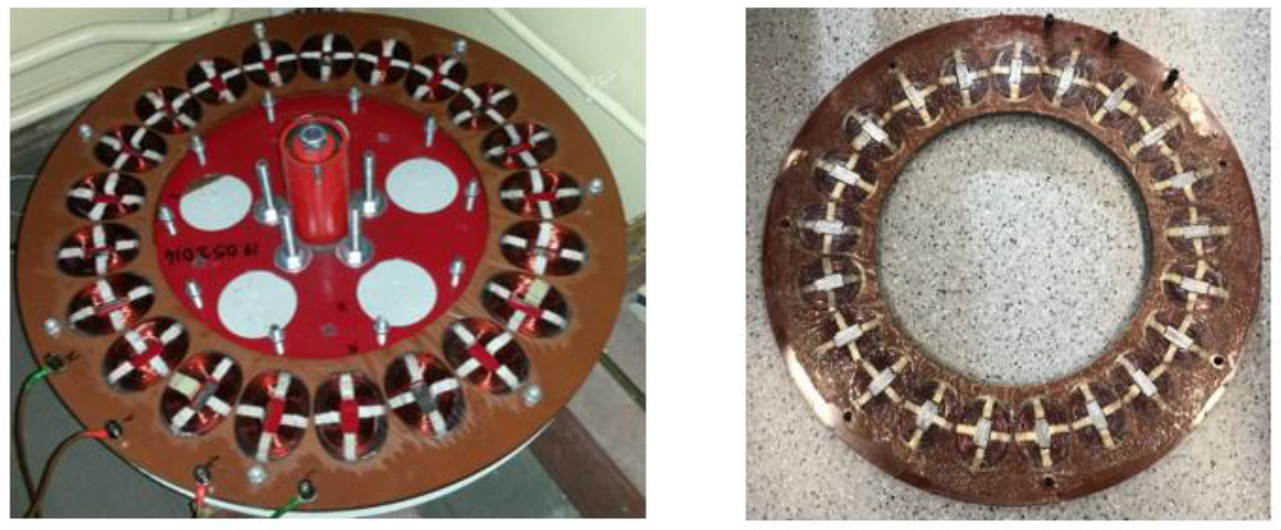
Construction of the stator in AFPM generator
  • R i = 270 mm; R o = 310 mm; r s = 290 mm;
  • l c = 40 mm; a c = 50 mm; a sc = 30 mm; l δ = 26 mm;
  • l i = 15 mm–for stator structure with cores
  • w s = 980; p s = 7 ; α sc ( r s ) = 0.1034 rad; ε ( r s ) = 0.1517 rad
  • R s = 2 Ω
Table 2. Comparison of the results obtained from analytical models and laboratory tests for THD factors of EMF.
AFPMGTHDE
Analytical CalculationsMeasure
G1Single magnets; coreless stator6.1%6.5%
G2Oblique magnets; coreless stator2.0%2.2%
G3Single magnets; stator with cores6.0%7.3%
G4Oblique magnets; stator with cores1.3%1.9%
Table 3. Comparison of the results obtained from analytical models and laboratory tests.
AFPMGEG (RMS)IG (RMS)
Analytical MeasureEG (%)|Analytical MeasureIG (%)|
G1Simple magnets; coreless stator 61.3 V62.6 V2.1%1.65 A1.69 A2.4%
G2Skewed magnets; coreless stator 101.5 V105.1 V3.4%2.42 A2.46 A1.6%
G3Simple magnets; stator with cores101.3 V95.8 V5.7%2.29 A2.23 A2.6%
G4Skewed magnets; stator with cores143.4 V140.9 V1.8%3.52 A3.43 A2.6%
Publisher’s Note: MDPI stays neutral with regard to jurisdictional claims in published maps and institutional affiliations.

