Abstract
The corrosion behavior of pure aluminum (Al) in 20 v/v% ethanol–gasoline blends has been studied using electrochemical techniques. Ethanol was obtained from different fruits including sugar cane, oranges, apples, or mangos, whereas other techniques included lineal polarization resistance, electrochemical noise, and electrochemical impedance spectroscopy for 90 days. Results have shown that corrosion rates for Al in all the blends were higher than that obtained in gasoline. In addition, the highest corrosion rate was obtained in the blend containing ethanol obtained from sugar cane. The corrosion process was under charge transfer control in all blends; however, for some exposure times, it was under the adsorption/desorption control of an intermediate compound. Al was susceptible to a localized, plotting type of corrosion in all blends, but they were bigger in size and in number in the blend containing ethanol obtained from sugar cane.
1. Introduction
Engines that use gasoline and alcohol as renewable energy sources have gained relevance lately and have been the subject of intense research studies all over the world. Due to its high octane number, ethanol has been extensively used either as an additive to gasoline or as another fuel instead of fossil fuel, leading to a number of research works dealing with both engine performance and pollution. However, alcohol absorbs water because it is highly hygroscopic and shows ethanol impurities (i.e., organic acids, esters, and ketones), which makes metallic materials that come in contact with ethanol–gasoline highly susceptible to corrosive attacks [1,2,3]. Numerous studies have been undertaken to evaluate the corrosion behavior of metallic materials used in components of vehicle fuel systems [4,5,6,7,8,9,10,11,12,13,14,15,16,17]. Bahena et al. [18] evaluated the corrosion behavior of four metals, including pure aluminum, chromium steel carbon steel, and copper in a 20% ethanol-80–gasoline blend using both weight loss and electrochemical impedance spectroscopy. They found that carbon steel and copper exhibited a greatest corrosion rate. Similarly, Yoo et al. studied the corrosion behavior of A384 aluminum alloy in bio-ethanol blended gasoline with 10, 15, and 20% of ethanol at 60, 80, and 100 °C using electrochemical impedance spectroscopy [19]. They found that the corrosion rate increased with an increase in the ethanol contents, and the lowest value was found at 80 °C. The type of corrosion was a plotting type. In a similar work carried out by Park et al. [20] with the same alloy in the same environment, it was found that acetic acid increased the alloy corrosion rate but water enhanced the formation of protective corrosion products, which led to a decreasing corrosion rate of the alloy. Finally, in a similar study [21], Jafari et al. evaluated the effect of ethanol contents (0, 5, 10, and 15%) and the addition of water with gasoline on the corrosion behavior of 304 type stainless steel, low/high carbon steel, aluminum, copper, and brazing alloy by using electrochemical impedance spectroscopy. They found that the corrosion rate in all tested alloys increased when ethanol contents increase. However, the addition of water increased the corrosion rate in ferrous metals, whereas the opposite behavior was observed for the nonferrous alloys. Metals were susceptible to a uniform type of corrosion, either in the presence or absence of water. No localized types of corrosion were observed in any specimen. Thus, the goal of the present study was to evaluate the effect of the ethanol source on the corrosion behavior of pure Al in a 20% ethanol–gasoline blend by using different electrochemical techniques. Herein, we used different sources of ethanol, such as sugar cane, oranges, apples, or mangos.
2. Experimental Procedure
2.1. Synthesis of Ethanol
Ethanol is most commonly produced by the fermentation of fruits. In this study, we produced ethanol via sugar cane, oranges, apples, or mangos, which were obtained by standard fermentation procedures. All fruits were obtained in a local market. Herein, we used the following substrates: modified Yellow Prussiate of Soda (YPS) with 250 g/L, KH2PO4 (99.3%, Sigma) 1 g/L, MgSO4.7H2O (99%, J.T. Baker) 0.5 g/L, peptone frm Bacto (Becton, Dickinson) 10 g/L, and yeast (Oxoid, Hampshire) 5 g/L. Sugar content was determined using the dinitrosalicylic acid method, whereas saccharose was determined via hydrolysis with 10% HCl al 10% at 95 °C. The ethanol quantification process was performed using gas chromatography (Agilent 300 A). To determine water content, 10 g of ethanol was weighed in glass tubes (in triplicate) that were previously dried in a muffle and weighed. After one hour at 105 °C in a forced convection oven, samples were removed and placed in a desiccator for 20 min at room temperature. Then, the samples were weighed. The procedure was repeated until a constant weight value was obtained. To determine the water content, the following formula was used:
where w is the initial weight (sample + tube), w1 is the weight after drying (sample + tube), and w2 is the sample weight.
2.2. Fourier Transform Infrared Spectroscopy (FTIR) Analysis
A Perkin–Elmer FTIR system was used to study the obtained ethanol by analyzing the attenuated total reflectance (ATR) under a ZnSe crystal in a range 4000 cm−1 to 650 cm−1. Commercial gasoline was used as a reference and was mixed with the different ethanol.
2.3. Electrochemical Measurements
Employed electrochemical techniques had open circuit potential (OCP), specifically electrochemical impedance spectroscopy (EIS) and electrochemical noise (EN). For this purpose, a potentiostat from ACM instruments was used. By using a standard glass cell, a graphite rode was used as the auxiliary electrode, where a saturated calomel electrode (SCE) was the reference electrode and aluminum (Al) bars with a surface area of 0.32 cm2 were used as working electrodes. Before carrying the experiments, specimens were abraded with 1200 grade emery paper, degreased with acetone, and rinsed with deionized water. For the EN measurements, the current between the working electrode and another nominally identical working electrode were taken. Moreover, the potential noise was taken versus the SCE reference electrode in blocks of 1024 points. EIS measurements were taken with the application of a signal of 30 mV around the free corrosion potential value, Ecorr, in a frequency range of 0.05–20,000 Hz. Experiments lasted 90 days at room temperature, which was around 25 °C.
2.4. Surface Characterization
Specimens that corrode surfaces were investigated using a LEO brand, model 1450 VP scanning electron microscope (SEM) (ZEISS, Jena, Germany).
3. Results and Discussion
3.1. Infrared Results and Chemical Composition
FTIR results of the obtained alcohols are shown in Figure 1, whereas the water content of different obtained ethanols are given in Table 1. This table shows that the water content was higher for the ethanol made from sugar cane than ethanol obtained from oranges, apples, or mangos, which affected corrosion results. Ethanol purity was higher than 99%, according to Table 1. Figure 1 clearly shows that the four alcohols displayed a virtually identical FTIR spectrum to a different intensity for different functional groups. The hydroxyl group was identified by its bending vibration, which was found with an intense and wide signal at 3370 cm−1. There was evidence that a hydroxyl group was found from an alcohol group at 1053 and 594 cm−1. The presence of CH3- and CH2-OH groups were evident at 2887 and 2972 cm−1, respectively, whereas those for CH2- and C-OH are found at 1647 and 1040 cm−1. All signals were more intense in the mango ethanol.
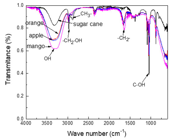
Figure 1.
Fourier transform infrared spectroscopy (FTIR) spectra for the different obtained ethanols.

Table 1.
Water and oxygen contents for the different obtained ethanols.
3.2. OCP Measurements
The effect of the ethanol source on the variation of the OCP value with time for Al in the different ethanol–gasoline blends are shown in Figure 2. The noblest values were obtained in pure gasoline, due to its high resistivity, as well as its low water and oxygen solubility. On the other hand, the most active OCP value was obtained in the blend made with ethanol obtained from sugar cane, which was probably due to higher water and oxygen contents. The OCP values obtained in the blends made with ethanol from oranges and mangos were very noble; however, after 30 days of exposure, their values became more active. A similar trend was observed for the OCP values obtained for the blend made with ethanol obtained from apples. The shift towards more active values was probably due to the dissolution of any air formed from the oxide layer, whereas the shift into the noble direction was due to the formation of corrosion product layers after metal dissolution [22].
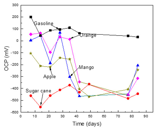
Figure 2.
Variation on the open circuit potential (OCP), value for Al in the different ethanol–gasoline blends.
3.3. LPR Measurements
Time variation for polarization resistance, Rp, in different ethanol–gasoline blends is given in Figure 3. Corrosion current density values, Icorr, can be calculated by using following equation:
where K is a constant that involves cathodic and anodic Tafel slopes obtained from polarization curves not obtained in this study due to the high solution resistivity values. Figure 3 shows that the lowest Rp values, and thus the highest Icorr values, were obtained for the blend made with the ethanol obtained from sugar cane. The Rp obtained in blends made with ethanols obtained from either oranges, apples, or mangos were higher by at least two orders of magnitude than those obtained in the blend made with sugar cane ethanol. The highest Rp values, and thus the lowest Icorr values, were obtained from pure gasoline, due to its low water and oxygen affinity [21]. However, in all cases, regardless of the ethanol source, Rp values had erratic behavior with time, since sometimes it increased and other times it decreased.
Icorr = K/Rp
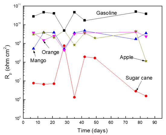
Figure 3.
Variation on the Rp value for Al in the different ethanol–gasoline blends.
The increase in the Rp value was a result of the accumulation of a corrosion product layer on the metal surface, whereas a decrease on its value was a result of the detachment of this corrosion product layer. According to Rawat et al. [23], the oxygen contents in pure gasoline was 0, whereas in sugar cane the ethanol was 34.7 wt. %. In a 20% ethanol–gasoline blend, this decreased to 7.0. Similarly, water solubility in pure gasoline was 0, whereas in ethanol it was 100%. Yet in the 20% ethanol–gasoline blend this value was between 0.5 and 0.7%. Thus, the difference in Rp values and, therefore, in the corrosion rates, were a result of a difference in both oxygen content and water solubility value in the different ethanol sources. In the same research work [23], Rawat et al. evaluated the effect of different ethanol–gasoline blends on the corrosion rate of different metals, including carbon steel, copper, and brass. In all cases, regardless of the metal chemical composition, they found that the corrosion rate increased with the ethanol contents due to an increase in both oxygen content and water solubility value.
3.4. Electrochemical Noise Measurements
The spontaneous fluctuations in both potential and current density values of a metal in an electrolyte (i.e., its electrochemical noise) was a powerful tool to determine the susceptibility of that metal for a localized type of corrosion, such as plotting [24]. As an example of these fluctuations, the time series in both the current density and potential density 84 days after exposure in a blend containing ethanol made from sugar cane are given in Figure 4. For day 1, the time series consisted of a combination of low intensity and high frequency transients, with some other transients with a slightly higher intensity but much lower frequency, indicating a metal undergoing a localized type of corrosion [25,26]. The intensity was around 10−8 mA/cm2 for the transients in the current density and 0.02 mV for the transients in the potential density, respectively. However, after 84 days of exposure, the frequency of transients with a higher intensity increased, since the intensity for these transients was 10−6 mA/cm2, which indicated a higher susceptibility to a localized type of corrosion. By dividing the standard deviation in the potential density, δV, by the standard deviation in the current density, δI, we could calculate the noise resistance, Rn, as stated below:
Rn = δV/ δI
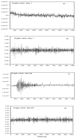
Figure 4.
Noise in current and in potential for Al in the blend containing ethanol obtained from sugar cane after ((a) and (b)) 1 day and ((c) and (d)) 84 days of exposure.
The variation on the Rn value with time in the different ethanol–gasoline blends are given in Figure 5. The lowest Rn value was, once again, for the tests carried out in the blend with the ethanol made from sugar cane, whereas the highest values were obtained in pure gasoline, similar to the results given by Rp in Figure 4. Thus, different techniques give similar results, which was encouraging, as it confirmed that the highest corrosion rates were obtained in the blends made with ethanol obtained from sugar cane.
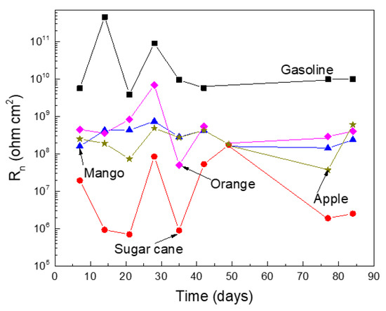
Figure 5.
Variation on the Rn value for Al in the different ethanol–gasoline blends.
In order to have a quantitative estimation of the metal susceptibility to localized corrosion, a factor called the “localized index”, LI, can be calculated by dividing the root mean square value of the current density, Irms, by the standard deviation in the current density, δI, according to:
Rn = Irms/δI
Obtained results are given in Figure 6. Metal had a high propensity to suffer from the localized type of corrosion when the LI value were between 0.1 and 1, where it would suffer from a uniform mixture and localized corrosion type if its value were between 0.01 and 0.1. Results shown in Figure 6 indicate that Al was highly susceptible to a localized type of corrosion, such as plotting, in all the ethanol–gasoline blends regardless of the ethanol source. For the blend containing ethanol made from sugar cane, these results indicated that Al could develop a mixture of localized and uniform type of corrosion.
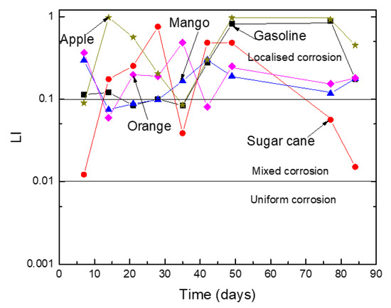
Figure 6.
Variation on the LI value for Al in the different ethanol–gasoline blends.
3.5. Electrochemical Impedance Spectroscopy (EIS) Measurements
EIS data in both the Nyquist and Bode formats for Al corroding in the ethanol–gasoline blend that contained ethanol made from mango during 90 days of exposure are given in Figure 7.
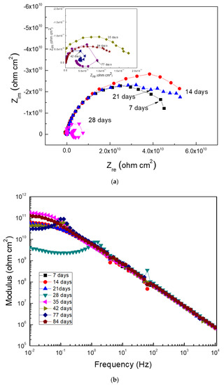
Figure 7.
Electrochemical impedance spectroscopy (EIS) data in the (a) Nyquist and (b) Bode formats for Al in the blend containing ethanol obtained from mangos.
Data plotted in the Nyquist diagram shows a charge-transfer control since it observed one capacitive semicircle at all frequency values (Figure 7a). However, in some cases such as at 28, 42, and 77 days of exposure, an inductive loop at low frequency values appeared, which showed that the corrosion process was controlled by the adsorption/desorption of some intermediate compounds. The Bode diagram, shown in Figure 7b, indicated that the impedance modulus sometimes increased or decreased with time, which was indicative of the formation of the corrosion product layer and its detachment. The presence of two different slopes in this plot was also evident, thus indicating the presence of two time constants. Thus, in Nyquist plots, there were two different semicircle: one, at high and intermediate frequency values, due to the redox reactions that took place at the metal/corrosion products layer, and a second semicircle at lower frequency values, due to the redox reactions that took place at the metal/electrolyte interface (the double electrochemical layer). According to the Bode plot, the highest impedance modules were within the order of 1010 ohm cm2, which was similar to the Rp and Rn values reported above in Figure 4 and Figure 5.
Figure 8 shows EIS data in the Nyquist and Bode formats for Al that corroded in the ethanol–gasoline blend containing ethanol made from sugar cane 90 days after exposure. Nyquist diagrams (Figure 8a) display one capacitive semicircle at high and intermediate frequency values, whereas at lower frequencies an unfinished capacitive semicircle was observed, indicating a charge transfer controlling corrosion process. The observed loop at the high frequency semicircle represented the redox reactions that took place at the metal/corrosion product layer, whereas the low frequency loop represented the electrochemical reactions that took place at the metal/electrolyte (double electrochemical layer) interface. This time, the presence of inductive loops was not observed as in the ethanol–gasoline blend containing ethanol made from mangos (Figure 7a). Bode plots (Figure 8b) show that the impedance modulus decreased with an increase in exposure time and presence of two different slopes, suggesting two different time constants: one for the electrochemical reactions that took place at the double electrochemical layer, and a second one for the electrochemical reactions that took place through the corrosion product layer. It is important to note that the impedance values were within the order of 106 ohm cm2, which was much lower than those obtained for Al in the blend containing ethanol made from mangos, similar to the Rp and Rn values given in Figure 4 and Figure 5.
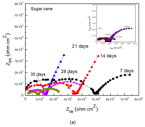
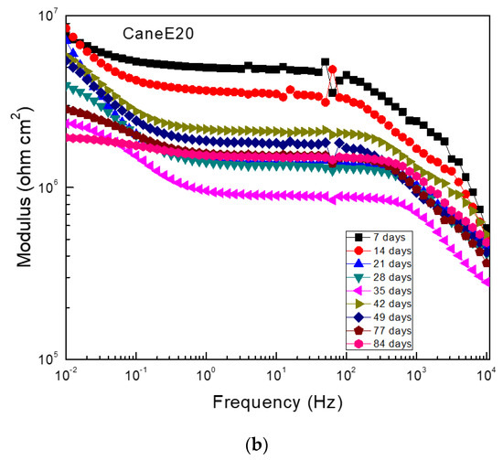
Figure 8.
EIS data in the (a) Nyquist and (b) Bode formats for Al in the blend containing ethanol obtained from sugar cane.
For Al corroding in the ethanol–gasoline blend containing ethanol made from apples, Nyquist data (Figure 9a) shows the presence of one capacitive semicircle at high and intermediate frequency values, overlapped with a second capacitive loop at the lowest frequency values; the high frequency loop was associated with the redox reactions that took place at the metal/corrosion product film, whereas the lowest frequency loop was related to the redox reactions that took place at the metal/electrolyte interphase or double electrochemical layer, indicating that the corrosion process was under charge transfer control. On the other hand, Bode plots (Figure 9b) show that the impedance modulus sometimes increased or decreased with time, indicating the formation of a corrosion products film detached from the corrosion product film. Two different slopes were observed in the modulus-frequency plots, which was indicative of two different time constants. The impedance values were within the order of 1010 ohm cm2, which was similar to the Rp and Rn values given in Figure 4 and Figure 5.
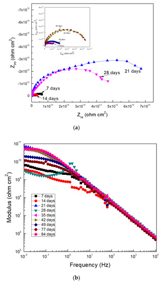
Figure 9.
EIS data in the (a) Nyquist and (b) Bode formats for Al in the blend containing ethanol obtained from apples.
Finally, Figure 10 presents the Nyquist and Bode plots for Al corroding in the ethanol–gasoline blend containing ethanol made from oranges. The Nyquist diagrams (Figure 10a) show a single capacitive semicircle in the whole frequency interval, i.e., a corrosion process controlled by the charge transfer reaction; however, the presence of two slopes were observed in the Bode plots (Figure 10b). Thus, the two time constants indicated that there were two different capacitive loops: one at high and intermediate frequency values, which was associated with the electrochemical reaction that took place at the metal/corrosion product film, and a second capacitive low frequency loop, which was associated with the electrochemical reaction that took place at the metal/electrolyte interface or double electrochemical layer. However, after 35, 42, and 77 days of exposure, an inductive loop at the lowest frequency values following the high frequency loop was observed, indicating that the corrosion process was controlled by the adsorption/distortion of some intermediate species. Bode plots also showed that the impedance modulus values, in general terms, increased as time increased due to the formation of corrosion product films, and the existence of two different time constants: one corresponding to the electrochemical reactions that took place at the metal/corrosion products film, and a second one representing the electrochemical reactions that took place at the metal/electrolyte interphase or double electrochemical layer.
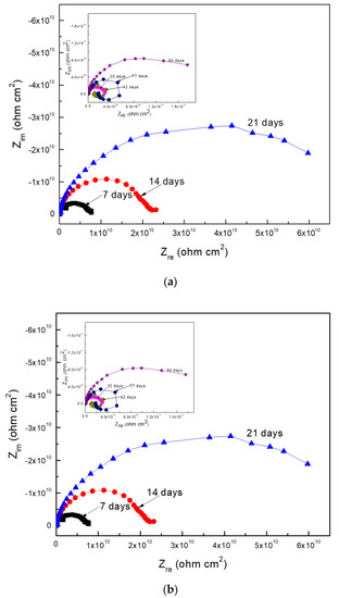
Figure 10.
EIS data in the (a) Nyquist and (b) Bode formats for Al in the blend containing ethanol obtained from oranges.
Electric circuits are commonly used to simulate EIS results and. in this case, the ones that had the best fit are shown in Figure 11, As such, their elements had a solution resistance, Rs, and charge transfer resistance, Rct, associated with the double electrochemical layer. Moreover, Cdl was the double layer capacitance that was inversely proportional; Rf had corrosion product film resistance and Cf was its capacitance; L was the inductor and RL its resistance. Polarization resistance, Rp, was the sum of all of these resistances, i.e., Rs + Rct + Rf. The double layer and corrosion products film capacitance value, Cdl and Cf, were affected by surface imperfections, such as roughness, which were made instead of a pure double layer capacitor, Cdl, when a constant phase element, CPE, was used [27]. The impedance of CPE, ZCPE, is given by [28]:
where is the admitance, is (−1)1/2, is the angular frequency, and n is the CPE exponent that gives information on the metal surface such as metal roughness (Figure 11). Obtained parameters that best fit the Nyquist and Bode results of Al after 7 days of exposure to the different ethanol–gasoline blends by using electric circuits are shown in Figure 11 and Table 2.
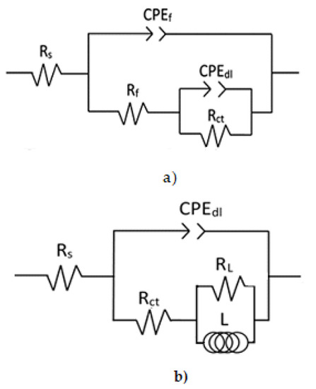
Figure 11.
Electric circuits used to simulate EIS data for Al in ethanol–gasoline blends when the corrosion process is under (a) cage transfer and (b) adsorption/desorption control.
Table 2.
Parameters used to fit the EIS data for Al corroding in the different ethanol–gasoline blends after 7 days of exposure.
The first important thing to note is the high solution resistance values, Rs, within the order of 104 ohm cm2 regardless of the ethanol source. The second thing to note is that the values for Rf are always higher than those for Rct, indicating that the corrosion resistance of Al in the different blends is given by the protectiveness of the corrosion product film. The lowest values for Rf and Rct were obtained in the blend containing ethanol made from sugar cane, indicating that, in this blend, Al exhibited the highest corrosion rate as given by Equation (1) above, in agreement with the results obtained in the LPR and electrochemical noise measurements (Figure 4 and Figure 5). Since the capacitance was inversely proportional to the resistance value, an increase in the resistance value corresponded to a decrease in its capacitance. When the values for n were close to 1.0, a low metal surface roughness had a low dissolution rate. On the contrary, when it was close to 0.5, it was because of a high surface roughness due to a high dissolution rate. According to data given in Table 1, values for both nct and nf were within 0.8 and 0.9 for the tests carried out in blends containing ethanol obtained from oranges, apples, or mangos, due to a low surface roughness because the corrosion rate of Al in these blends was low. On the contrary, the values for both nct and nf were 0.6 and 0.7 for the tests carried out in the blend containing ethanol obtained from sugar cane due to a high surface roughness because the corrosion rate of Al in this blends was high. Thus, all the test suggest that the blend containing ethanol obtained from sugar cane was more aggressive for Al than the blends containing ethanol obtained from oranges, apples, or mangos, which may be a result of higher water and oxygen content.
3.6. Surface Characterization
Figure 12 shows micrographs of Al corroded surfaces after 90 days of exposure to different ethanol blends. For the test done in pure gasoline, specimens did not show any type of attack, as can be seen in Figure 12a; however, for the tests carried out in blends containing ethanol made from oranges, apples, or mangos, some shallow plots with a size smaller than 10 μm could be seen. Even more, for the test carried out in the blend containing ethanol made from sugar cane (Figure 12d), the plot size was larger than 40 μm and deeper than those observed in other blends. Nonetheless, it was very likely that it was a coalescence of several smaller plots. Thus, these micrographs were in agreement with all the electrochemical tests results, i.e., that Al did not suffer from any type of corrosion attack in pure gasoline; that the ethanol made from oranges, apples, or mangos were more aggressive than pure gasoline; and that ethanol made form sugar cane was the most aggressive among the different ethanol tested in this research work, perhaps because of its higher oxygen and water contents than those in the rest of the ethanol obtained from oranges, apples, or mangos.
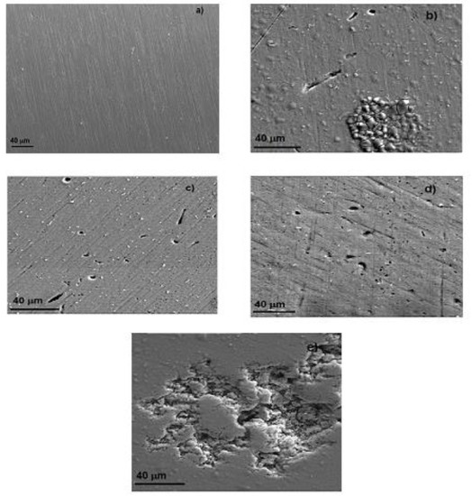
Figure 12.
Micrograph of Al corroded in (a) gasoline and in ethanol–gasoline blends containing ethanol made from (b) apples, (c) mangos, (d) oranges, and (e) sugar cane.
4. Discussion
The most widely used form to explain Al corrosion in ethanol–gasoline blends was the electrochemical process produced by water and dissolved oxygen, which enhanced cathodic reactions due to phase separation [28]. Oxygen was introduced as an automotive fuel that could produce better engine performance, whereas ethanol was oxidized by this dissolved oxygen to form water plus acetic acid [29].
C2H5OH + O2 →CH3COOH + H2O
Acetic acid corroded Al not in an electrochemical way, but in a chemical way that produced hydrogen gas and aluminum acetate [30]:
Al + CH3COOH → 3/2H2 + Al(CO3COO)3
Water either facilitates aqueous conditions that enhance corrosion processes, or forms protective layers of corrosion products, such as bayerite (Al(OH)3) or boehmite (AlOOH) [30]. This film can be disrupted in some localized places or, due to the amount of water and oxygen present in the blend, it does not cover the whole Al surface, inducing a localized type of corrosion, such as the observed plots. The protective nature of these films depends upon the presence of impurities such as chlorides, sulfates, and other organic compounds that depend on the source of the ethanol, among other factors. Due to the different nature of the obtained ethanol, the presence of these impurities must be different to explain the diverse effects they have on Al corrosion behavior.
5. Conclusions
In this study, we conducted an investigation on the corrosion behavior of pure Al in 20% ethanol–gasoline blends using electrochemical techniques that contained ethanol obtained from sugar cane, oranges, apples, or mangos. Each technique showed that corrosion rates obtained in the blends were higher than that obtained in gasoline. However, corrosion rates were highest in the blend containing ethanol obtained from sugar cane. The corrosion process was controlled by the charge transfer in all the blends regardless of the ethanol source; however, for some exposure times, it was under the adsorption/desorption of an intermediate compound. Although Al was susceptible to the localized type of corrosion in all blends, plots were much bigger and deeper in the blend containing ethanol obtained from sugar cane.
Author Contributions
Conceptualization, J.G.G.-R.; methodology, A.B.-F. and S.A.S.-B.; software, R.L.-S. and J.A.H.-P.; validation, C.R.-V. and I.R.-C.; formal analysis, J.U.; investigation, A.B.-F.; resources, S.A.S.-B.; data curation, J.A.H.-P; writing—original draft preparation, J.G.G.-R.; writing—review and editing, C.R.-V.; visualization, I.R.-C.; supervision, J.U.; project administration, A.B.-F.; funding acquisition, J.G.G.-R. All authors have read and agreed to the published version of the manuscript.
Funding
This research was funded by CONACYT Mexico under grant number 827388.
Acknowledgments
Authors want to thank René Guardian Tapia in providing the SEM images.
Conflicts of Interest
The authors declare no conflict of interest.
References
- Von Blottnitz, H.; Curran, M.A. A review of assessments conducted on bio-ethanol as a transportation fuel from a net energy, greenhouse gas, and environmental life cycle perspective. J. Clean. Prod. 2007, 15, 607–619. [Google Scholar] [CrossRef]
- Tibaquirá, J.E.; Huertas, J.I.; Ospina, S.; Quirama, L.F.; Niño, J.E. The Effect of Using Ethanol–gasoline Blends on the Mechanical, Energy and Environmental Performance of In-Use Vehicles. Energies 2018, 11, 221. [Google Scholar] [CrossRef]
- Xiaoyuan, L.; Singh, P.M. Cathodic activities of oxygen and hydrogen on carbon steel in simulated fuel-grade ethanol. Electrochim. Acta 2011, 56, 2312–2320. [Google Scholar]
- De souza, J.P.; Mattos, O.R.; Sathler, L.; Takenouti, H. Impedance measurements of corroding mild steel in an automotive fuel ethanol with and without inhibitor in a two and three electrode cell. Corros. Sci. 1987, 27, 1351–1364. [Google Scholar] [CrossRef]
- Scholz, M.; Ellermeier, J. Corrosion behavior of different aluminum alloys in fuels containing ethanol under increased temperatures. Mater. Werkst. 2006, 37, 842–851. [Google Scholar] [CrossRef]
- Eppel, K.; Scholz, M.; Troßmann, T.; Berger, C. Corrosion of metals for automotive applications in ethanol blended biofuels. Energy Mater. 2008, 3, 227–231. [Google Scholar] [CrossRef]
- Del-Pozo, A.; Torres-Islas, A.; Villalobos, J.C.; Sedano, A.; Martínez, H.; Campillo, B.; Serna, S. Stress corrosion cracking of microalloyed pipeline steel in biofuels E-10 and E-85. Corros. Eng. Sci. Technol. 2019, 54, 37–45. [Google Scholar] [CrossRef]
- Jafari, H.; Idris, M.H.; Ourdjini, A.; Rahimi, H.; Ghobadian, B. Effect of ethanol as gasoline additive on vehicle fuel delivery system corrosion. Mater. Corros. 2010, 61, 432–440. [Google Scholar]
- Dimatteo, A.; Lovicu, G.F.; Desanctis, M.; Valentini, R.; Santarelli, S.; Cognetta, F. Compatibility of nickel and silver-based brazing alloys with E85 fuel blends. Mater. Corros. 2015, 66, 158–168. [Google Scholar] [CrossRef]
- Aperador, W.; Caballero-Gómez, J.; Delgado, A. Corrosion Behavior of the AA2124 Aluminium Alloy Exposed to Ethanol Mixtures. Int. J. Electrochem. Sci. 2013, 8, 6154–6161. [Google Scholar]
- Pedraza-Basulto, G.K.; Arizmendi-Morquecho, A.M.; Cabral Miramontes, J.A.; Borunda-Terrazas, A.; Martinez-Villafane, A.; Chacón-Nava, J.G. Effect of Water on the Stress Corrosion Cracking Behavior of API 5L-X52 Steel in E95 Blend. Int. J. Electrochem. Sci. 2013, 8, 5421–5437. [Google Scholar]
- Liu, C.; Frankel, G.S.; Sridhar, N. Effect of Oxygen on Ethanol Stress Corrosion Cracking Susceptibility: Part 1—Electrochemical Response and Cracking-Susceptible Potential Region. Corrosion 2013, 69, 768–780. [Google Scholar]
- Sridhar, N. Knowledge-Based Predictive Analytics in Corrosion. Corrosion 2018, 74, 181–196. [Google Scholar] [CrossRef]
- Skoropinski, D.B. Corrosion of aluminum fuel system components by reaction with EGME icing inhibitor. Energy Fuel 1996, 10, 108–116. [Google Scholar] [CrossRef]
- Yoo, Y.H.; Park, I.J.; Kim, J.G.; Kwak, D.H.; Ji, W.S. Corrosion characteristics of aluminium alloy in bio-ethanol blended gasoline fuel: Part 1. The corrosion properties of aluminum alloy in high temperature fuels. Fuel 2011, 90, 633–639. [Google Scholar] [CrossRef]
- Cavalcanti, E.; Wanderley, V.G.; Miranda, T.R.V.; Uller, L. The effect of water, sulphate and pH on the corrosion behavior of carbon steel in ethanolic solutions. Electrochim. Acta 1987, 32, 935–947. [Google Scholar] [CrossRef]
- Monteiro, M.R.; Ambrozin, A.R.P.; Santos, A.O.; Contri, P.P.; Kuri, S.E. Evaluation of metallic corrosion caused by alcohol fuel and some contaminants. Mater. Sci. Forum 2010, 636, 1024–1029. [Google Scholar] [CrossRef]
- Baena, L.M.; Gomez, M.; Calderon, J.A. Aggressiveness of a 20% bioethanol–80% gasoline mixture on auto parts: I behavior of metallic materials and evaluation of their electrochemical properties. Fuel 2012, 95, 320–328. [Google Scholar] [CrossRef]
- Yoo, Y.H.; Park, I.J.; Kim, J.G.; Kwak, D.H.; Ji, W.S. Corrosion characteristics of aluminium alloy in bio-ethanol blended gasoline fuel: Part 2. The effects of dissolved oxygen in the fuel. Fuel 2011, 90, 1208–1214. [Google Scholar] [CrossRef]
- Hassan, J.; Idris, M.H.; Ourdjini, A.; Rahimi, H.; Ghobadian, B. EIS study of corrosion behavior of metallic materials in ethanol blended gasoline containing water as a contaminant. Fuel 2011, 90, 1181–1187. [Google Scholar]
- Olafsen, A.; Fjellvag, H. Synthesis of rare earth oxide carbonates and thermal stability of Nd2O2CO3. J. Mat. Chem. 1999, 9, 2697–2702. [Google Scholar] [CrossRef]
- Rawat, J.; Rao, P.V.C.; Nettem, V.C. Effect of Ethanol–gasoline Blends on Corrosion Rate in the Presence of Different Materials of Construction used for Transportation, Storage and Fuel Tanks. Open Electrochem. J. 2009, 1, 32–36. [Google Scholar]
- Turgoose, S.; Cottis, R.A. Corrosion Testing Made Easy: Electrochemical Impedance and Noise; NACE International: Houston, TX, USA, 1999; pp. 1–149. [Google Scholar]
- Hladky, K.; Dawson, J.L. The measurement of localized corrosion using electrochemical noise. Corros. Sci. 1981, 21, 317–322. [Google Scholar] [CrossRef]
- Hladky, K.; Dawson, J.L. The measurement of corrosion using electrochemical 1/f noise. Corros. Sci. 1982, 22, 231–237. [Google Scholar] [CrossRef]
- Bommersbach, P.; Alemany-Dumont, C.; Millet, J.P.; Normand, B. Hydrodynamic effect on the behavior of a corrosion inhibitor film: Characterization by electrochemical impedance spectroscopy. Electrochim. Acta 2006, 51, 4011–4018. [Google Scholar] [CrossRef]
- Behpour, M.; Ghoreishi, S.M.; Salavati-Niasari, M.; Ebrahimi, B. Evaluating two new synthesized S–N Schiff bases on the corrosion of copper in 15% hydrochloric acid. Mater. Chem. Phys. 2008, 107, 153–157. [Google Scholar] [CrossRef]
- French, R.; Malone, P. Phase equilibria in ethanol fuel blends. Fluid Phase Equilib. 2005, 229, 27–40. [Google Scholar] [CrossRef]
- MArinov, N. A detailed chemical kinetic model for ethanol oxidation. Int. J. Chem. Kinet. 1999, 31, 183–220. [Google Scholar] [CrossRef]
- Vargel, C. Corrosion of Aluminum; Elsevier Ltd.: Oxford, UK, 2004; pp. 1–120. [Google Scholar]
Publisher’s Note: MDPI stays neutral with regard to jurisdictional claims in published maps and institutional affiliations. |
© 2020 by the authors. Licensee MDPI, Basel, Switzerland. This article is an open access article distributed under the terms and conditions of the Creative Commons Attribution (CC BY) license (http://creativecommons.org/licenses/by/4.0/).