Abstract
The aging of rechargeable batteries, with its associated replacement costs, is one of the main issues limiting the diffusion of electric vehicles (EVs) as the future transportation infrastructure. An effective way to mitigate battery aging is to act on its charge cycles, more controllable than discharge ones, implementing so-called battery-aware charging protocols. Since one of the main factors affecting battery aging is its average state of charge (SOC), these protocols try to minimize the standby time, i.e., the time interval between the end of the actual charge and the moment when the EV is unplugged from the charging station. Doing so while still ensuring that the EV is fully charged when needed (in order to achieve a satisfying user experience) requires a “just-in-time” charging protocol, which completes exactly at the plug-out time. This type of protocol can only be achieved if an estimate of the expected plug-in duration is available. While many previous works have stressed the importance of having this estimate, they have either used straightforward forecasting methods, or assumed that the plug-in duration was directly indicated by the user, which could lead to sub-optimal results. In this paper, we evaluate the effectiveness of a more advanced forecasting based on machine learning (ML). With experiments on a public dataset containing data from domestic EV charge points, we show that a simple tree-based ML model, trained on each charge station based on its users’ behaviour, can reduce the forecasting error by up to 4× compared to the simple predictors used in previous works. This, in turn, leads to an improvement of up to 50% in a combined aging-quality of service metric.
1. Introduction
Given the environmental impact of petroleum-based transportation and the recent developments of renewable energy production technologies, electric vehicles (EVs) are gaining traction as the most promising transportation infrastructure for the future [1]. EVs are considered environmental-friendly because the electric power they consume can be generated from a wide variety of sources including various renewable ones [2]. Using renewables for transportation has the potential to massively reduce fuel consumption and gas emissions as well as increase the security level of energy usage, via geographic diversification of the available sources. In addition to protecting the environment, EVs also have advantages in terms of higher energy efficiency and lower noise than internal combustion engines [3].
Although EVs are currently ordinary in most sectors of public and private transportation, with rapidly growing market demands, one critical issue that still limits their adoption is related to batteries. There is an urgent demand for advanced battery optimization strategies that can satisfy customers’ demands, such as increasing the driving range and reducing the charge time, while also containing the costs associated with battery replacement [4]. In fact, the battery is the main contributor to the total cost of an EV, accounting for more or less 75% of the total capital cost of the full vehicle [5]. Thus, prolonging the lifetime of the battery becomes a crucial issue in the development of EVs.
Since two decades, Lithium-ion has become the dominant battery chemistry adopted in EVs due to its relatively high energy density and power delivery ability [6]. Among the weaknesses of Lithium-ion technology, capacity loss is one of the essential aspects that influences EVs’ widespread adoption [7]. The aging of a Lithium-ion battery, intended as the loss of usable capacity over time, strongly affects the battery replacement cost. The aging of the battery depends on several quantities such as temperature, depth of discharge (DOD), average state of charge (SOC), and magnitude of the charge/discharge currents [8,9,10]. The values of these quantities during the discharge phase (in particular the DOD and the discharge current) cannot be controlled because they depend on the motor power demand, which in turn is a function of the EV driving profile, and therefore is determined by user habits. In contrast, the charge phase is more controllable and as such provides some space for battery aging optimization.
EV battery charging is usually constrained to use standardized schemes, based on pre-defined current and voltage profiles. Because of the low cost and straightforward implementations, constant current-constant voltage (CC-CV) charge protocol is the most common one for Lithium-ion batteries. The CC-CV protocol effectively limits the risk of overcharging, which has to be carefully managed in Lithium-ion batteries. Although constraining to CC-CV does limit the space for optimizations, this protocol still offers some degrees of freedom (namely, the charge starting time and the charge current) that can be leveraged to mitigate aging [10,11,12,13,14,15,16,17].
As a matter of fact, vehicles are often connected to a charge station for a time much longer than what is needed to charge their battery, that is, the plug-in duration is often much longer than the actual charge duration. The default charge scheme starts the CC phase as soon as the vehicle is plugged in, using a large current to obtain a fast charge. While this solution yields a 100% charged battery as fast as possible, it can significantly degrade the battery capacity. This fast capacity loss is due to a twofold effect. The first direct cause is that battery aging worsens with large charge currents. Moreover, according to the default charge protocol, charging is typically completed well before the actual plug-out time. This early completion implies a higher average SOC stored in the battery, which also negatively affects the aging [8]. Therefore, there exists a trade-off between (fast) charge time and battery aging: the former requires larger charge currents and an immediate start of the charging protocol at plug-in time, both of which degrade battery capacity.
Several works in the literature have proposed aging-aware charging protocols that try to overcome the limitations of this default solution [10,11,12,13,14,15,16,17]. To do so, these protocols jointly optimize the final charge state of the battery in each charge cycle and its aging. Both objectives have to be considered since, paradoxically, the ideal policy for aging-only optimization would otherwise coincide with leaving the battery fully discharged (0 charge current and SOC), which is clearly not meaningful. In contrast, the charge state of the battery at plug-out time is fundamental for the EV driver’s user experience. In practice, these approaches optimize the two free parameters of the CC-CV protocol (start time and charge current) in such a way that the battery becomes fully charged exactly when it is plugged out of the charge station.
To this end, an estimate of the plug-in duration is needed. The accuracy of such an estimate is fundamental, as pointed out in [17]. Indeed, overestimating the plug-in duration would cause the battery to have a low SOC at plug-out time, dramatically degrading user experience. On the other hand, overestimating it would worsen the battery aging as charging would complete before the actual plug-out time, increasing the average SOC. Despite the importance of accurate plug-in duration estimation, previous works have only relied on elementary models. Several works [10,11,13] assume that the plug-in duration is set directly by the user when plugging the EV into the station. In those approaches, the responsibility of providing an accurate estimate is entirely left to the user, who mostly cares about the driving experience rather than battery aging. Other approaches, although not targeting EV batteries specifically, attempt an automatic estimate [12,17], but only using basic models such as fixed-time predictions or moving averages.
In this work, we assess the effectiveness of using a machine learning (ML) model in improving the accuracy of plug-in duration estimation. Our approach is based on the observation that, especially for domestic stations, plug-in and plug-out instants depend on the habits of a single user (or a small group). Therefore, we envision a system in which each charge station autonomously learns its users’ plug-in behaviour from history. With experiments on a public dataset containing records from domestic charge stations in the UK [18], we show that a simple tree-based model (light gradient boosting or LightGBM) can reduce the prediction error compared to all straightforward policies considered in previous work. Using this model on top of an aging-aware charging protocol, in turn, yields an improvement of up to 54% on a combined quality-of-service/aging metric. Moreover, the accuracy of the ML predictor is strongly related to the number of records present in the dataset for a given charge station, suggesting that even better results could be achieved with more available data.
In summary, our main contributions are the following:
- We evaluate for the first time the effectiveness of a ML-based approach for predicting the plug-in duration of EVs in domestic charge stations.
- We show that this method is superior in terms of prediction accuracy with respect to the straightforward policies used by previous works.
- Finally, we show that this reduction of the prediction error actually translates into an improvement in terms of quality-of-service and battery aging, when the prediction is used within an aging-aware EV charging protocol.
The rest of the paper is organized as follows. Section 2 provides the required background on battery charging and aging models, and discusses related works; Section 3 describes the different plug-in duration estimates considered in our experiments. Section 4 reports the results, while Section 5 concludes the paper.
2. Background and Related Works
2.1. EV Battery Capacity Aging Degradation
The capacity loss of rechargeable Lithium-ion batteries depends on four main factors [8,13,19,20]: (i) temperature, (ii) DOD at each cycle (also referred to as deviation of the SOC), (iii) average SOC, and (iv) charge/discharge current. Aging worsens with an increase in any of these quantities.
Among these four main factors, given that temperature cannot be easily controlled and that DOD and discharge currents depend on the power demand and duration of the discharge phase, only the charging current and the average SOC can be managed during the charging process for optimization.
The average SOC for a generic time interval from to , is given by:
For instance, [19] reports that, for LiFePO4 batteries, SOC should be less than 60% on average for maintaining battery life acceptable.
Aging is usually evaluated through the state of health (SOH) aggregate metric, defined as the ratio of the capacity of an aged battery and its nominal capacity. In this work, since we focus on multiple charge cycles, we need a model that expresses the aging for each cycle. To this purpose we use the classical model of [19] augmented as in [13] to account for charge and discharge current. The following expression determines battery capacity loss (L) in the i-th cycle:
where is the battery aging factor provided by the Millner’s model [19], which accounts for temperature, deviation of the SOC, and SOC in the i-th cycle; and is the battery aging computed by the model provided by [13], which strengthen the Millner’s model by adding aging dependence on discharge and charge current values in the i-th cycle, and . and are empirical coefficients extracted from battery datasheet information [13] or from experimental measurements. By summing over M cycles, we get the total loss of capacity . and SOH are both normalized, so they are related as SOH . The SOH after M-th cycle is therefore indicated by:
This model can be applied to any device powered with Lithium-ion type batteries, and supports battery aging estimation after multiple cycles. Therefore, it can be used to identify charging protocols that best fit a specific user behavior from the point of view of both battery aging and quality of service (QoS).
In this work, we use the average SOC at plug-out time as a metric of QoS, since the available residual capacity at the plug-out time determines the quality of user experience. Mathematically:
This metric is commonly used [10,17], since a higher SOC at the plug-out time guarantees a longer driving range and a better driving experience (e.g., allowing the enabling of auto-auxiliary driving system, on-board multi-media systems, etc.), and vice-versa.
2.2. EV Battery Charging with CC-CV
Charging a battery is an operation that may significantly impact its lifetime, even more than discharging when comparing the effects of the same absolute current rate in both phases [9]. Selecting the appropriate charge protocol is thus a critical step, not only for keeping as much as possible unaltered the battery performance, but also for avoiding dangerous side effects, like overheating and overcharging, which besides creating obvious hazards, can also worsen the battery SOH, defined in (3) and accelerate the battery aging.
The selection of the proper charge scheme depends on the battery chemistry. For Lithium-ion batteries (the majority of EVs are equipped with this kind of battery cells), the standard is to adopt the CC-CV protocol [21]. Although various optimized charging methods were explored and reported in the literature (e.g., [15,22]), CC-CV is still adopted in the great majority of Lithium-ion battery-based systems, due to the simplicity of chargers implementations from an electrical point of view, and because it guarantees battery safety against over-voltage and over-current.
The CC-CV protocol operates in three phases, as shown in Figure 1. In the first phase (CC), the battery is charged at a constant current until its voltage reaches a pre-determined limit; in the second phase (CV), the battery is charged at a constant voltage until the current drops to a pre-defined value. This second phase effectively manages the risk of overcharging, which is quite dangerous in Lithium-ion batteries. The time interval starting after the end of the second phase until to the unplug time is called standby time. As shown in Figure 1, the SOC remains fixed at 100% in this third phase, which is detrimental for the SOH of Lithium-ion batteries, since the length of standby period significantly increases the average SOC of the battery. An analytical macro-model of CC-CV charge time based on a subset of all relevant parameters, namely, average SOC, deviation of the SOC (here considered as depth-of-discharge), discharge/charge current, and temperature is presented in [23].
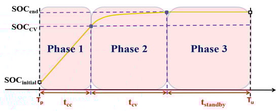
Figure 1.
Typical CC-CV charging protocol scenario.
In this work, we evaluate the impact of an accurate plug-in duration estimation on aging-aware charging protocols that stick to the CC-CV scheme, and only act on the free parameters made available by it. As explained in [10,17] these free parameters are the starting time and the slope (which depends on the current) of the first phase of Figure 1, i.e., the CC phase.
Solutions that remain compliant with CC-CV do so in order to maintain its electrical simplicity, low cost and safety properties, while still adapting the standard to consider battery aging. In our work, considering these solutions allows us to assess the impact of our plug-in duration forecasting on realistic charge stations most commonly used nowadays. However, our method is actually orthogonal to a specific charging profile, and could therefore be used also in conjunction with advanced aging-aware schemes that do not follow the CC-CV standard [9,14,15,16].
2.3. Aging-Aware Charging Protocols
As anticipated, most of the previous works on aging-aware charging of Lithium-ion batteries focus on altering two main CC-CV protocol variables, namely the average SOC (shortening length of Phase 3 in Figure 1) and the constant charging current (decreasing the slope of the line in Phase 1 of Figure 1). The two approaches are schematized in Figure 2.
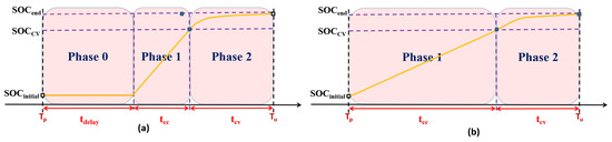
Figure 2.
Aging-aware charging protocols: (a) Delay the charge starting time to reduce the average SOC; (b) Decrease the charging current in CC phase.
In terms of the SOC effect on aging, the charge phase should ideally reach 100% exactly at unplug time (see Figure 2a); this would yield the smallest possible average SOC, minimizing the length of the standby period, while still guaranteeing a fully charged battery, which corresponds to the best QoS [12]. In contrast, when charging is started immediately at the plug-in time, batteries are often left fully charged for a long time, as indicated by the in Figure 1, with a significant impact on battery aging [8]. The work in [12] was one of the firsts to consider delayed start time for charging batteries as late as possible, thus minimizing the average SOC.
Concerning the charge current, Ref. [11] mitigates battery aging by considering only this parameter, and calculating a minimum current that ensures a fully charged battery at the end of a predicted plug-in period, whenever it is higher than the charge time needed in standard CC-CV. In [16], the non-linear relation between charge current and charging time is analyzed.
In [13], both charge current and average SOC are taken into account. The authors show that the aging-optimal charge current is more related to battery usage rather than plug-in time, and that the capacity loss vs. charge current characteristic is not monotonic. However, their aging analysis is limited to a single cycle, and the actual plug-in time is assumed to be known.
A CC-CV compliant charge protocol that takes into account all the relevant parameters is proposed in [17]. Because of the opposing goals of obtaining a fully charged EV and optimizing battery aging, Ref. [17] uses a QoS metric based on the deviation from 100% charge level at plug-out time. Results are then reported in a 2-dimensional aging/QoS space to represent the trade-off between these two quantities. With this multi-objective analysis, it is shown that the proposed protocol obtains a better trade-off under various user charge/discharge pattern statistics compared to [13], which only considers aging at the expense of low QoS. Although both [13,17] focus on the Lithium-ion batteries found in mobile devices (such as smartphones), the proposed charging protocols are general and can be applied to any battery-powered device, including EVs.
Finally, other works have proposed aging-aware charge protocols that however do not stick to the CC-CV scheme [14,15,16].
Importantly, many recent works [10,11,12,13,17] analyze the need for predicting the plug-in duration by extracting the data from battery usage history; however, no accurate prediction mechanisms are proposed. For example, Ref. [17] calculates the optimal charge current based on a simple prediction of the plug-in duration to achieve a “just-in-time” charge. Although this work gives a detailed analysis of the effect of plug-in duration forecasting, it only uses a simple predictor based on an exponential moving average (EMA) to estimate the current cycle’s plug-in duration. The few simple predictors proposed in literature are used as baselines for comparison in our experiment, and are detailed in Section 3.3.
The recent work of [24] proposed an intelligent charging solution to prolong the lifetime of battery-powered devices. Also this work underlines the importance of plug-out time prediction (Notice that, since the plug-in time is known at the beginning of each charging phase, estimating the plug-in duration or the plug-out time is equivalent, and we use both terms interchangeably in the paper) accuracy for alleviating the aging of battery during charging phase. It suggests using multiple data sources and connecting multiple battery-powered intelligent devices to increase the accuracy of predictions and to allocate charging power intelligently among different devices. Unfortunately, this work only lists the need of accurate prediction as an open challenge for designing intelligent EV chargers, and no specific forecasting model is proposed.
2.4. Machine Learning Applications in EVs
Machine learning is used in many other applications related to EVs and to battery-related optimizations. Among the most relevant ones is driving range estimation [4,25,26], which has been addressed, among others, using ML models based on linear regression [26] and self-organizing maps [25]. ML based on deep neural networks has also been used to optimize the energy requested by EVs in a demand-side management framework [27]. Finally, other applications of ML models to EVs include engine faults diagnosis [28] and estimation of the battery State-of-Charge (SOC) [29] and State-of-Health (SOH) [30]. Notice that the latter are different and orthogonal to the goal of this work. In fact, our aim is estimating the plug-in time, which is then used to guide a battery-aware charging protocol. In turn this determines the SOC and the SOH of the battery, which can be estimated either with the analytical models described in Section 2.1 or with the ML methods of [31,32]. To the best of our knowledge, ML-based approaches have never been used for plug-in duration estimation.
3. Methods
The objective of our work is to build a reliable predictor of the plug-in duration of an EV onto a domestic charging station. Specifically, we want to assess whether a ML solution does yield superior prediction accuracy compared to the basic prediction policies used by previous works, which we take as comparison baselines. Then, we want to assess whether this superior accuracy corresponds to a sizeable improvement in the QoS/aging space for the EV battery. To this end, we apply our ML-based prediction, as well as the baselines, on top of the As Soon As Possible (ASAP) and Aging-Optimal battery-aware CC-CV protocols described in [13,17]. We briefly describe the two protocols in Section 4.1 and refer the readers to the original papers for more details. As anticipated, our predictor is independent of the underlying charge protocol; nonetheless, testing with these two state-of-the-art protocols allows us to assess its real impact on battery aging and QoS.
In the rest of this section, we first describe the scenario in which we envision to deploy our ML-based forecasting in Section 3.1. We then detail the selected ML algorithm in Section 3.2 and the comparison baselines in Section 3.3.
3.1. Continuous Charge Behaviour Learning with Edge Computing
In the target scenario, plug-in time forecasting (i.e., ML inference) must be performed at the beginning of each EV charging phase, in order to let the charge station implement an optimized protocol which needs this information as input. Moreover, once the charge cycle ends, the real plug-in duration becomes known. In case of a ML approach, this new information should be used to update the prediction model, so that the system continuously learns from the users’ charging behaviours. This strategy can allow significant improvements in prediction accuracy over time [33]. However, it also implies that, at the end of each charge cycle, a re-training of the ML model should be executed.
Modern EV charge stations include either a central processing unit (CPU) or a micro-controller unit (MCU) [34], normally used to monitor the charging, provide alerts and feedback to the user, etc. One option could be to use this processing device just for collecting historical data of past charging phases (e.g., a record containing plug-in time, plug-out time, day of the year, etc. for each charge cycle), and then offload all the processing to a cloud server [35]. However, this solution requires the availability of a cloud infrastructure, and that the charge station is constantly connected to the Internet. Moreover, transmitting EV charging records over the Internet may also raise security concerns, as these data might be intercepted by malicious third parties and used to infer private information about users’ behaviours (e.g., when they are at home or not) [36]. As an alternative to this approach, we propose a solution based on edge computing, where the ML algorithm is directly executed in the charge station processing hardware [35,36]. The two alternatives are schematized in Figure 3.
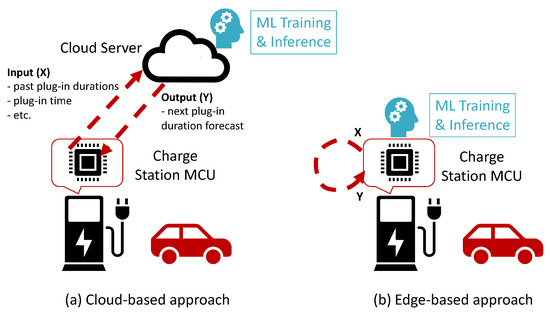
Figure 3.
Alternative scenarios for the deployment of ML-based plug-in duration forecasting.
As shown in the Figure, the edge-based solution solves all aforementioned problems, but it introduces new limitations to the characteristics of the selected ML algorithm. In fact, processors present in EV charging stations (e.g., from the ARM Cortex family) are normally designed for embedded applications. While these devices are sufficiently powerful to implement simple ML-based predictors, their compute power (number of cores, clock frequency, available memory) is significantly more limited than what is available on a cloud server [35,37]. This is especially critical since, as anticipated, both training and inference should be performed repeatedly. Therefore, computational complexity for the training and inference phases of the model becomes a key design metric. For this reason, complex models such as deep neural networks [38], although possibly very accurate, are not a viable option. In contrast, we select light gradient boosting (LightGBM) [39] to implement our ML-based predictor. LightGBM models are based on tree learning, and are explicitly designed to limit the computational complexity for training (i.e., tree growing), as detailed in the following section.
3.2. Light Gradient Boosting
LightGBM is a type of ML model belonging to the gradient boosting family, and it is based on ensembles of trees. It was first proposed by [39] in 2017.
In our work, we decided to focus on tree-based learning since it is inherently one of the most efficient types of ML in terms of both inference and training complexity. In fact, performing inference (i.e., classification or regression) on an input datum simply requires performing a set of comparisons with thresholds, one for each visited tree node [40]. Therefore, the number of operations performed in an inference is , where is the depth of the m-th tree and M the number of trees in the ensemble. Similarly, the number of parameters (i.e., thresholds) of the model is , where is the total number of nodes in the m-th tree. Comparisons are very simple operations from a hardware point of view, which makes this type of inference easy to implement even on micro-controllers [40]. In addition to maintaining this inference simplicity, LightGBM extends the standard gradient boosting decision tree (GBDT) algorithm [41] with several optimizations that speed-up its training time up to 20 times. Moreover, tree-based learning is also effective when training set sizes are not extremely large [42], as in the case of the dataset described in Section 4. In such a “small-data” setting, other models, such as deep learning ones, which are extremely accurate in general, would likely lead to over-fitting and therefore to poor results [43].
Considering the training set of a supervised learning problem , both GBDT and LightGBM build predictions in the form:
where is a decision tree, also called weak learner and is a weight. The goal of training is to minimize the expected value of a loss function , such as the squared error loss in the case of regression problems [44]:
As in standard GBDT, also in LightGBM weak learners are trained sequentially one after the other, and each tree learns to predict the negative residual error (or gradient) from previous models. In mathematical terms, negative residuals are computed as:
where the second equality comes from the squared error loss in (6). The m-th tree is then grown using the training set . Finally, the corresponding weight is computed as:
In terms of complexity, the most critical step of this training procedure is the growth of individual trees. In LightGBM, trees are grown leaf-wise, as shown in Figure 4. As explained in [39], this requires operations for each expansion, where is the number of features in each input sample .
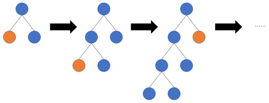
Figure 4.
Leaf-wise tree growth in LightGBM.
LightGBM reduces this computational burden by sub-sampling training data and bundling features. The first objective is achieved thanks to a technique called gradient-based one-side sampling (GOSS): when growing the m-th tree, GOSS samples the training instances considered for split-point selection based on the magnitude of their gradient , computed as in (7). Specifically, the training instances with largest gradient are always selected, whereas of the remaining instances are randomly sampled. The values of a and b are hyper-parameters of the algorithm. The authors of [39] show that are sufficient to obtain good accuracy, while significantly speeding up training time. LightGBM combines GOSS with so-called exclusive feature bundling (EFB), an optimization which further reduces the training time by “bundling” mutually-exclusive features (i.e., those that are never simultaneously ). While EFB is very effective in general [39,44], it is less relevant than GOSS for our work, since we train our LightGBM predictor using few and not mutually exclusive features (see Section 4).
In our experiments, we retrain the LightGBM model after each EV charge cycle, using as training data all past history until that moment. For simplicity, the model is currently retrained from scratch every time. However, we plan to also experiment with incremental learning techniques for GBDT-like models, such as those proposed in [45] in our future work, to further speed-up training time.
3.3. Baseline Algorithms
Previous works on aging-aware Li-ion battery charging schemes have almost always assumed the plug-in duration as a known input. The few exceptions, such as [12,17] have used simple time-series predictors such as the exponential moving average (EMA) and the historical average (HA). Therefore, to the best of our knowledge, ours is the first work to utilize a proper ML algorithm for plug-in duration forecasting. Accordingly, in our experiments, we have compared the proposed LightGBM predictor with the following four simple baselines.
3.3.1. Fix Duration and Fix Time
It is not easy to compare the ML-based solution against a scenario in which the EV users directly indicate the predicted unplug time when they leave the car at the charge station (as assumed in [10,11,13]). In fact, the behaviour of each vehicle user is different. Nonetheless, we can use two simple predictors called Fix Duration and Fix Time to mimic two common categories of behaviours.
The Fix Duration prediction always assumes a fixed plug-in duration , regardless of any other condition (plug-in time, day of the week, etc.). In our experiments, we have tried setting to 6 h, 8 h and 12 h. The best results have been obtained with 6.
The slightly more complex Fix Time predictor, instead, assumes that the unplug time of the EV always occurs at one of two possible fixed times of the day and . This is similar to a user-specified “alarm-like” unplug prediction. Specifically, if the EV is plugged in at time t where this predictor assumes that the unplug time is . Conversely, if it assumes that the EV will be unplugged at , where this value refers to the next day if the second condition is verified. The predicted plug-in duration is then computed as the difference between the predicted unplug time and t. Mathematically:
This predictor takes as its only input the latest plug-in time t. Using two different fixed times allows to account for EV charges happening both during the day and during the night, a common pattern as pointed out in [10]. In our experiments, we tried different combinations of and , and achieved the best results using 7.00 a.m. and 7.00 p.m. respectively.
3.3.2. Exponential Moving Average
This baseline is taken from the works of [12,17] which, although targeting smartphone batteries rather than EVs’, proposed to estimate the unplug time using an exponential moving average (EMA). The estimated plug-in duration at cycle i is therefore computed as:
where is the actual (measured) plug-in duration at the previous charge cycle, and is a smoothing weight. EMA-based forecasting assumes that consecutive charge cycles have a similar duration; as such, most of the estimate depends on the latest measurement, while the previous history is accounted for by the second addend. This prediction does not depend on the plug-in instant, like (9), and only uses the previous plug-in duration as an input.
3.3.3. Historical Average
The historical average (HA) is different from the EMA in that it gives equal importance to the entire past history of plug-in duration measurements.In this case, the predicted duration is simply computed as the average of all past measurements, i.e.,:
This predictor is used in previous work by [12]. Again, the only required input for this forecasting strategy is the set of past plug-in duration.
4. Results
4.1. Experimental Setup
The methods described in Section 3, have been applied to the publicly available “Electric Chargepoint Analysis: Domestics” dataset, collected by the United Kingdom’s office for low emission vehicles (OLEV) [18]. This dataset contains records of charging events from approximately 25,000 domestic charge-points across the UK, collected during the year 2017, for a total of 3.2 million charging events. Each charging record contains the dates and times of the start and end of the plug-in, as well as the acquired energy in KW, the plug-in duration, the charge point identifier, and the charge event identifier. Our experiments have been performed on 5 charging points with identifiers AN05770, AN10157, AN23533, AN08563, and AN03003, selected based on the large number of available charging events (see Table 1). We did not generalize our results to the entire dataset because the great majority of the charging points contain a very limited number of charging event records, which are not sufficient to train the proposed LightGBM model. Before training the predictors, all charge events longer than 40 h have been filtered out as outliers (e.g., holidays), since we have found that they worsened the training results.

Table 1.
Number of charge events in each considered station.
Both the LightGBM predictor and the comparison baselines are trained and tested on individual charge points, in order to simulate the scenario described in Section 3.1. The first 65% of the total events in each charge station have been used as initial training set, and the predictors have been evaluated on the remaining 35%.
As reported in Table 2, as inputs for the LightGBM model, we used the following features for each charging event: the plug-in date and time, expressed as day of the year, hour and minute; the day of the week of plug-in, encoded using a one-hot format, in order to account for different charging patterns during the week and on the weekend; the plug-in duration of the previous charge cycle; the plug-out date and time of the previous charge cycle. LightGB algorithm parameters have been tuned using grid search on each charge station. We also tried feeding the LightGBM model with a longer past history, but we empirically found out that this led to overfitting (i.e., a reduction of the forecasting error on the training set but an increase on the test set) and therefore worsened the performance of the model when used within an aging-aware battery charging protocol.
Table 2.
Input features for the LightGBM model.
Plug-in duration predictors have been written in Python, using the LightGBM package [46] for the proposed model. Battery discharge and charge cycles simulations have been performed in MATLAB. We selected the A123 Systems ANR26650M1A automotive Lithium-ion battery in our simulations. All the necessary parameters of its aging model to compute the in (2) are provided in [19], whereas the related discharge and charge current rate coefficients, and in (2) are extracted from [13]. The environment temperature in our simulations is set as 25 °C and the battery operating temperature is assumed as a constant value equal to 35 °C. To simulate the charging phase, we adopted the model of [36], which supports changing the current values and computing the length of CC and CV phases. The maximum and minimum CC phase charging currents have been set to 0.1C rate and 2C rate in the aging-aware charging protocols.
The EV discharge behaviour cannot be inferred from the dataset. So, it has been modeled using the same method of [10]. For each charge station, the simulations relative to different forecasting methods have been fed with the exact same sequence of discharge profiles, so that the comparison among them is fair. For what concerns the charge phase, which is the main focus of this work, as anticipated in Section 3, we inserted the different plug-in duration forecasting algorithms in two aging-aware CC-CV-based charging protocols. The first one, which we refer to as Aging-Optimal, was proposed in [13] and works by delaying the charging start time and simultaneously reducing the charging current. Moreover, we also consider the as soon as possible (ASAP) protocol of [17], which starts charging immediately and only reduces the charging current. Both of them need an accurate prediction of the plug-out time to determine the optimal charging current in the CC phase or its starting time. We remark that designing an aging and/or QoS optimal charging protocol is not the target in this work. We test on these two aging-aware charging protocols just to illustrate the importance of plug-in duration prediction accuracy.
4.2. Forecasting Error
As a first experiments, the proposed model and the baselines have been compared in terms of pure prediction error. For this, the mean square error (MSE) has been used as a target metric, defined as:
where y is the actual plug-in duration, is the forecast one and n is the number of plug-in events at a given charge point.
The results of this experiment are presented in Figure 5, which reports the MSE obtained by all forecasting methods for each of the five considered charge points. As shown, the LightGBM forecasting obtains the lowest error on all five stations.
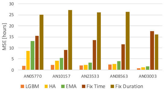
Figure 5.
Mean Square Error of the models.
Interestingly, the HA predictor is a close second for some stations, showing that the average plug-in duration is approximately constant over long periods. However, on average, LightGBM reduces the prediction error by 34% compared to HA. Moreover, the difference between the two methods is the largest for the charge point labeled AN05770, which is also the one with the most numerous charge cycles in the dataset (see Table 1). For that station, the error reduction of LightGBM with respect to HA is >4×. This suggests that having more data for training allows the ML-based method to learn the subtleties of user EV charging behaviours, and consequently improve the forecasting accuracy compared to a simple predictor like HA. Figure 6a shows the actual plug-in duration in hours and the corresponding LightGBM prediction for the plug-in events of station AN05770; Figure 6b indicates the absolute error between our prediction and the real plug-in duration for each charge event; Figure 6c displays the histogram of the LightGBM prediction error. This example visually shows that the proposed ML-based predictor is able to provide an accurate estimate in most cases, with the largest errors happening in correspondence of outliers.
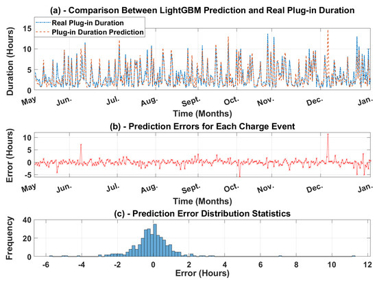
Figure 6.
Comparison between LightGBM prediction and actual plug-in duration (in hours) for charging point AN05770.
Aging and QoS Results
After verifying the performance of LightGBM forecasting, we inserted our proposed plug-in duration estimator into the two aging-aware charging protocols described in Section 4.1. According to previous works [17], we measured the performance of the charge protocols enhanced with the estimators on a 2-dimensional space. The impact of forecasting on battery aging has been measured using the SOH metric expressed in (3), whereas (4) was used to measure the QoS. Both SOH and QoS metrics are normalized between 0 and 1, with 1 corresponding to the ideal value.
Figure 7 and Figure 8 show the results of these simulations on the 2D metrics space. Optimality corresponds to the top-right corner of each chart, where both metrics have value 1. Table 3 reports the numerical results of these experiments. As shown, the proposed LightGBM always achieves the best QoS among all forecasting methods, for all stations and for both charging protocols. In terms of SOH, the ML-based prediction achieves slightly worse results than those obtained with the other methods, although still significantly better than those obtained by a standard (i.e., not aging-aware) CC-CV solution with no forecast. However, this demonstrates that pure aging-optimization without considering the QoS is meaningless. Indeed, looking only at the SOH axis, the Fix Duration prediction would be the best. However, this approach yields extremely low QoS values, ranging from 30% to less than 10%, which means that, using this solution, drivers would find their EV still almost fully discharged when they take it from the station.
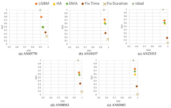
Figure 7.
Battery aging (SOH) versus QoS using different plug-in duration predictors and the Aging Optimal charge protocol from [13].
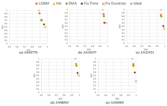
Figure 8.
Battery aging (SOH) versus QoS using different plug-in duration predictors and the ASAP charge protocol from [17].
Table 3.
MSE, QoS and SOH results using different plug-in duration predictors and the ASAP and Optimal charging protocols.
To better show this aspect, in Figure 7 and Figure 8 we have also plotted the result achieved by an Ideal predictor, i.e., an oracle algorithm that always knows the actual plug-in duration. As shown in the figures, this perfect predictor would also yield a slightly worse battery aging, in exchange for a perfect QoS (always 100% SOC at unplug time). The proposed LightGBM is therefore closer to an ideal forecast in all experiments. Interestingly, the HA method is significantly worse than LightGBM in terms of average QoS for some stations (e.g., AN05770 in Figure 7). This is probably due to the fact that, contrarily to LightGBM, once many training data become available, HA tends towards a constant prediction, and cannot adapt to changes in the user behaviour.
A quantitative way to compare the actual effectiveness of the different predictors using a single number is to measure how close they are to the optimal point in Figure 7 and Figure 8 or, equivalently, compute the product of the QoS and SOH metrics. This result is shown in Figure 9 and Figure 10, and in the rightmost columns of Table 3.
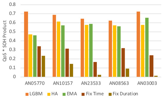
Figure 9.
QoS-SOH product using different plug-in duration predictors and the Aging Optimal charge protocol from [13].
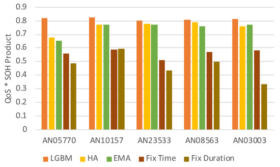
Figure 10.
QoS-SOH product using different plug-in duration predictors and the ASAP charge protocol from [17].
The graphs and table clearly show that the ML-based solution is superior to all baselines. On average, LightGBM improves the QoS-SOH product by 20% and 8% using the Aging Optimal and ASAP protocols respectively. Due to the lower prediction MSE, which in turn is a consequence of the larger amount of training data available, AN05770 is always the station for which the improvement is maximum, i.e., 54% and 21% respectively.
5. Conclusions
We have proposed a novel ML-based forecasting method to estimate the plug-in duration of EVs, and consequently improve the effectiveness of aging-aware charging protocols that need this information to implement a “just-in-time” charge. With experiments on a dataset containing real EV plug-in measurements from domestic charge stations, we have shown that this forecasting is superior to the basic approaches used in previous work, reducing the prediction error by 34% on average and up to 4×. Using our proposed predictor on top of two state-of-the-art aging-aware charging protocols, causes an improvement of their effectiveness, measured with a combined aging and user-experience metric, of 20% and 8% on average, and up to 54% and 21% respectively. Moreover, the fact that the largest improvements are always achieved for the charge station with the most records in the dataset suggests that even better results could be obtained with more data available. However, the availability of large public datasets to experiment on remains one of the biggest open challenges for this research. ML-based prediction of EVs plug-in duration may lead to a more cost-efficient use of batteries, and therefore help speed up the mass adoption of electric transportation. Moreover, these predictions could also be used to optimize load distribution and vehicle-to-grid solutions, to further improve the efficiency of smart grids. This analysis will be part of our future work.
Author Contributions
Conceptualization, Y.C., D.J.P., E.M. and M.P.; Data curation, K.S.S.A.; Investigation, Y.C. and D.J.P; Methodology, Y.C., D.J.P. and S.V.; Software, K.S.S.A.; Supervision, E.M. and M.P.; Writing—original draft, Y.C., K.S.S.A. and D.J.P; Writing—review & editing, S.V., E.M. and M.P. All authors have read and agreed to the published version of the manuscript.
Funding
This research received no external funding.
Conflicts of Interest
The authors declare no conflict of interest.
Abbreviations
The following abbreviations are used in this manuscript:
| EVs | Electric Vehicles |
| SOC | State Of Charge |
| ML | Machine Learning |
| DOD | Depth Of Discharge |
| CC-CV | Constant Current-Constant Voltage |
| LightGBM | Light Gradient Boosting |
| SOH | State Of Health |
| QoS | Quality of Service |
| EMA | Exponential Moving Average |
| HA | Historical Average |
| CPU | Central Processing Unit |
| MCU | Micro-controller Unit |
| GBDT | Gradient Boosting Decision Tree |
| GOSS | Gradient-based One-Side Sampling |
| EFB | Exclusive Feature Bundling |
| MSE | Mean Square Error |
References
- Zhang, Q.; Ou, X.; Yan, X.; Zhang, X. Electric vehicle market penetration and impacts on energy consumption and CO2 emission in the future: Beijing case. Energies 2017, 10, 228. [Google Scholar] [CrossRef]
- Eberle, U.; Von Helmolt, R. Sustainable transportation based on electric vehicle concepts: A brief overview. Energy Environ. Sci. 2010, 3, 689–699. [Google Scholar] [CrossRef]
- Yang, Z.; Shang, F.; Brown, I.P.; Krishnamurthy, M. Comparative study of interior permanent magnet, induction, and switched reluctance motor drives for EV and HEV applications. IEEE Trans. Transp. Electrif. 2015, 1, 245–254. [Google Scholar] [CrossRef]
- Baek, D.; Chen, Y.; Bocca, A.; Bottaccioli, L.; Cataldo, S.D.; Gatteschi, V.; Pagliari, D.J.; Patti, E.; Urgese, G.; Chang, N.; et al. Battery-Aware Operation Range Estimation for Terrestrial and Aerial Electric Vehicles. IEEE Trans. Veh. Technol. 2019, 68, 5471–5482. [Google Scholar] [CrossRef]
- Berckmans, G.; Messagie, M.; Smekens, J.; Omar, N.; Vanhaverbeke, L.; Van Mierlo, J. Cost projection of state of the art lithium-ion batteries for electric vehicles up to 2030. Energies 2017, 10, 1314. [Google Scholar] [CrossRef]
- Hannan, M.; Hoque, M.; Mohamed, A.; Ayob, A. Review of energy storage systems for electric vehicle applications: Issues and challenges. Renew. Sustain. Energy Rev. 2017, 69, 771–789. [Google Scholar] [CrossRef]
- Jafari, M.; Gauchia, A.; Zhang, K.; Gauchia, L. Simulation and analysis of the effect of real-world driving styles in an EV battery performance and aging. IEEE Trans. Transp. Electrif. 2015, 1, 391–401. [Google Scholar] [CrossRef]
- Barré, A.; Deguilhem, B.; Grolleau, S.; Gérard, M.; Suard, F.; Riu, D. A review on lithium-ion battery ageing mechanisms and estimations for automotive applications. J. Power Sources 2013, 241, 680–689. [Google Scholar] [CrossRef]
- Bashash, S.; Moura, S.J.; Forman, J.C.; Fathy, H.K. Plug-in hybrid electric vehicle charge pattern optimization for energy cost and battery longevity. J. Power Sources 2011, 196, 541–549. [Google Scholar] [CrossRef]
- Bocca, A.; Chen, Y.; Macii, A.; Macii, E.; Poncino, M. Aging and Cost Optimal Residential Charging for Plug-In EVs. IEEE Design Test 2017, 35, 16–24. [Google Scholar] [CrossRef]
- Matsumura, N.; Otani, N.; Hamaji, K. Intelligent Battery Charging Rate Management. U.S. Patent Application 12/059,967, 1 October 2009. [Google Scholar]
- Pröbstl, A.; Kindt, P.; Regnath, E.; Chakraborty, S. Smart2: Smart charging for smart phones. In Proceedings of the 2015 IEEE 21st International Conference on Embedded and Real-Time Computing Systems and Applications, Hong Kong, China, 19–21 August 2015; pp. 41–50. [Google Scholar]
- Bocca, A.; Sassone, A.; Macii, A.; Macii, E.; Poncino, M. An aging-aware battery charge scheme for mobile devices exploiting plug-in time patterns. In Proceedings of the 2015 33rd IEEE International Conference on Computer Design (ICCD), New York, NY, USA, 18–21 October 2015; pp. 407–410. [Google Scholar]
- Klein, R.; Chaturvedi, N.A.; Christensen, J.; Ahmed, J.; Findeisen, R.; Kojic, A. Optimal charging strategies in lithium-ion battery. In Proceedings of the 2011 American Control Conference, San Francisco, CA, USA, 29 June–1 July 2011; pp. 382–387. [Google Scholar]
- Shen, W.; Vo, T.T.; Kapoor, A. Charging algorithms of lithium-ion batteries: An overview. In Proceedings of the 2012 7th IEEE Conference on Industrial Electronics and Applications (ICIEA), Singapore, 18–20 July 2012; pp. 1567–1572. [Google Scholar]
- Guo, Z.; Liaw, B.Y.; Qiu, X.; Gao, L.; Zhang, C. Optimal charging method for lithium ion batteries using a universal voltage protocol accommodating aging. J. Power Sources 2015, 274, 957–964. [Google Scholar] [CrossRef]
- Chen, Y.; Bocca, A.; Macii, A.; Macii, E.; Poncino, M. A li-ion battery charge protocol with optimal aging-quality of service trade-off. In Proceedings of the 2016 International Symposium on Low Power Electronics and Design, San Francisco, CA, USA, 8–10 August 2016; pp. 40–45. [Google Scholar]
- Electric Chargepoint Analysis 2017: Domestics. Available online: https://www.gov.uk/government/statistics/electric-chargepoint-analysis-2017-domestics (accessed on 12 August 2020).
- Millner, A. Modeling lithium ion battery degradation in electric vehicles. In Proceedings of the 2010 IEEE Conference on Innovative Technologies for an Efficient and Reliable Electricity Supply, Waltham, MA, USA, 27–29 September 2010; pp. 349–356. [Google Scholar]
- Hoke, A.; Brissette, A.; Smith, K.; Pratt, A.; Maksimovic, D. Accounting for lithium-ion battery degradation in electric vehicle charging optimization. IEEE J. Emerg. Sel. Top. Power Electron. 2014, 2, 691–700. [Google Scholar] [CrossRef]
- Hussein, A.A.H.; Batarseh, I. A review of charging algorithms for nickel and lithium battery chargers. IEEE Trans. Veh. Technol. 2011, 60, 830–838. [Google Scholar] [CrossRef]
- Wang, Y.; Lin, X.; Xie, Q.; Chang, N.; Pedram, M. Minimizing state-of-health degradation in hybrid electrical energy storage systems with arbitrary source and load profiles. In Proceedings of the 2014 Design, Automation & Test in Europe Conference & Exhibition (DATE), Dresden, Germany, 24–28 March 2014; pp. 1–4. [Google Scholar]
- Shin, D.; Sassone, A.; Bocca, A.; Macii, A.; Macii, E.; Poncino, M. A compact macromodel for the charge phase of a battery with typical charging protocol. In Proceedings of the 2014 International Symposium on Low Power Electronics and Design, La Jolla, CA, USA, 11–13 August 2014; pp. 267–270. [Google Scholar]
- Pröbstl, A.; Islam, B.; Nirjon, S.; Chang, N.; Chakraborty, S. Intelligent Chargers Will Make Mobile Devices Live Longer. IEEE Des. Test 2020. [Google Scholar] [CrossRef]
- Zheng, B.; He, P.; Zhao, L.; Li, H. A Hybrid Machine Learning Model for Range Estimation of Electric Vehicles. In Proceedings of the 2016 IEEE Global Communications Conference (GLOBECOM), Washington, DC, USA, 4–8 December 2016; pp. 1–6. [Google Scholar]
- Sun, S.; Zhang, J.; Bi, J.; Wang, Y. A Machine Learning Method for Predicting Driving Range of Battery Electric Vehicles. J. Adv. Transp. 2019, 2019, 4109148. [Google Scholar] [CrossRef]
- López, K.L.; Gagné, C.; Gardner, M. Demand-Side Management Using Deep Learning for Smart Charging of Electric Vehicles. IEEE Trans. Smart Grid 2019, 10, 2683–2691. [Google Scholar] [CrossRef]
- Murphey, Y.L.; Masrur, M.A.; Chen, Z.; Zhang, B. Model-based fault diagnosis in electric drives using machine learning. IEEE/ASME Trans. Mechatron. 2006, 11, 290–303. [Google Scholar] [CrossRef]
- Chemali, E.; Kollmeyer, P.J.; Preindl, M.; Emadi, A. State-of-charge estimation of Li-ion batteries using deep neural networks: A machine learning approach. J. Power Sources 2018, 400, 242–255. [Google Scholar] [CrossRef]
- Vidal, C.; Malysz, P.; Kollmeyer, P.; Emadi, A. Machine Learning Applied to Electrified Vehicle Battery State of Charge and State of Health Estimation: State-of-the-Art. IEEE Access 2020, 8, 52796–52814. [Google Scholar] [CrossRef]
- Hu, X.; Li, S.E.; Yang, Y. Advanced Machine Learning Approach for Lithium-Ion Battery State Estimation in Electric Vehicles. IEEE Trans. Transp. Electrif. 2016, 2, 140–149. [Google Scholar] [CrossRef]
- Hu, X.; Jiang, J.; Cao, D.; Egardt, B. Battery Health Prognosis for Electric Vehicles Using Sample Entropy and Sparse Bayesian Predictive Modeling. IEEE Trans. Ind. Electron. 2016, 63, 2645–2656. [Google Scholar] [CrossRef]
- Xiao, J.; Xiong, Z.; Wu, S.; Yi, Y.; Jin, H.; Hu, K. Disk Failure Prediction in Data Centers via Online Learning. In Proceedings of the ICPP 2018 47th International Conference on Parallel Processing, Eugene, OR, USA, 13–16 August 2018; Association for Computing Machinery: New York, NY, USA, 2018. [Google Scholar] [CrossRef]
- Pate, M.; Ho, M.; Texas Instruments. Charging ahead toward an EV Support Infrastructure. Available online: https://www.ti.com/lit/wp/swpy030/swpy030.pdf (accessed on 12 August 2020).
- Chen, J.; Ran, X. Deep Learning With Edge Computing: A Review. Proc. IEEE 2019, 107, 1655–1674. [Google Scholar] [CrossRef]
- Shi, W.; Cao, J.; Zhang, Q.; Li, Y.; Xu, L. Edge Computing: Vision and Challenges. IEEE Internet Things J. 2016, 3, 637–646. [Google Scholar] [CrossRef]
- Jahier Pagliari, D.; Poncino, M.; Macii, E. Energy-Efficient Digital Processing via Approximate Computing. In Smart Systems Integration and Simulation; Bombieri, N., Poncino, M., Pravadelli, G., Eds.; Springer International Publishing: Cham, Switzerland, 2016; Chapter 4; pp. 55–89. [Google Scholar] [CrossRef]
- LeCun, Y.; Bengio, Y.; Hinton, G. Deep Learning; The MIT Press: Cambridge, MA, USA, 2006. [Google Scholar]
- Ke, G.; Meng, Q.; Finley, T.; Wang, T.; Chen, W.; Ma, W.; Ye, Q.; Liu, T.Y. LightGBM: A Highly Efficient Gradient Boosting Decision Tree. In Advances in Neural Information Processing Systems 30; Guyon, I., Luxburg, U.V., Bengio, S., Wallach, H., Fergus, R., Vishwanathan, S., Garnett, R., Eds.; Curran Associates, Inc.: Nice, France, 2017; pp. 3146–3154. [Google Scholar]
- Kumar, A.; Goyal, S.; Varma, M. Resource-efficient Machine Learning in 2 KB RAM for the Internet of Things. In Proceedings of the 34th International Conference on Machine Learning, Sydney, Australia, 6–11 August 2017; Precup, D., Teh, Y.W., Eds.; PMLR, International Convention Centre: Sydney, Australia, 2017; Volume 70, pp. 1935–1944. [Google Scholar]
- Li, F.; Zhang, L.; Chen, B.; Gao, D.; Cheng, Y.; Zhang, X.; Yang, Y.; Gao, K.; Huang, Z.; Peng, J. A light gradient boosting machine for remainning useful life estimation of aircraft engines. In Proceedings of the 2018 21st International Conference on Intelligent Transportation Systems (ITSC), Maui, HI, USA, 4–7 November 2018; pp. 3562–3567. [Google Scholar]
- Jiang, J.; Wang, R.; Wang, M.; Gao, K.; Nguyen, D.D.; Wei, G.W. Boosting Tree-Assisted Multitask Deep Learning for Small Scientific Datasets. J. Chem. Inf. Model. 2020, 60, 1235–1244. [Google Scholar] [CrossRef] [PubMed]
- Goodfellow, I.; Bengio, Y.; Courville, A. Deep Learning; The MIT Press: Cambridge, MA, USA, 2016. [Google Scholar]
- Sun, X.; Liu, M.; Sima, Z. A novel cryptocurrency price trend forecasting model based on LightGBM. Financ. Res. Lett. 2020, 32, 101084. [Google Scholar] [CrossRef]
- Zhang, C.; Zhang, Y.; Shi, X.; Almpanidis, G.; Fan, G.; Shen, X. On Incremental Learning for Gradient Boosting Decision Trees. Neural Process. Lett. 2019, 50, 957–987. [Google Scholar] [CrossRef]
- Python LightGBM Package. Available online: https://lightgbm.readthedocs.io/en/latest/ (accessed on 12 August 2020).
© 2020 by the authors. Licensee MDPI, Basel, Switzerland. This article is an open access article distributed under the terms and conditions of the Creative Commons Attribution (CC BY) license (http://creativecommons.org/licenses/by/4.0/).