Optimal Power Flow Management System for a Power Network with Stochastic Renewable Energy Resources Using Golden Ratio Optimization Method

Abstract

An optimal operation system is a potential solution to increase the energy efficiency of a power network equipped with stochastic Renewable Energy Sources (RES). In this article, an Optimal Power Flow (OPF) problem has been formulated as a single and multi-objective problems for a conventional power generation and renewable sources connected to a power network. The objective functions reflect the minimization of fuel cost, gas emission, power loss, voltage deviation and improving the system stability. Considering the volatile renewable generation behaviour and uncertainty in the power prediction of wind and solar power output as a nonlinear optimization problem, this paper uses a Weibull and lognormal probability distribution functions to estimate the power output of renewable generation. Then, a new Golden Ratio Optimization Method (GROM) algorithm has been developed to solve the OPF problem for a power network incorporating with stochastic RES. The proposed GROM algorithm aims to improve the reliability, environmental and energy performance of the power network system (IEEE 30-bus system). Three different scenarios, using different RES locations, are presented and the results of the proposed GROM algorithm is compared to six heuristic search methods from the literature. The comparisons indicate that the GROM algorithm successfully reduce fuel costs, gas emission and improve the voltage stability and outperforms each of the presented six heuristic search methods.

1. Introduction

1.1. Background

The using of Renewable Energy Sources (RES) in the electrical power network is increasing due to the need to reduce gas emissions fuel cost and increase energy efficiency [1,2,3]. RES such as solar and wind systems have a direct effect on electricity market and contribute in minimizing the power line losses, energy generation costs and improving the stability and reliability of power system. In addition, the location of RES in the grid have an influence on the performances of power network control and operation. As a result, the network operators will be forced to optimally control the conventional power generations and RES or change the way in which the energy has been consumed. The fuel cost, gas emissions and power loss and voltage deviation challenges in power networks can be translated to an Optimal Power Flow (OPF) problem, using RES with a number of operation constraints. The OPF problem’s formulation plays a vital role in operating modern power systems and it has been widely applied in different applications such as buildings, power networks and renewable energy [1,2,3]. In the literature, OPF has been used to select the parameters of power network control variables to achive the proposed objective function for the problem. The OPF studies for power networks [4,5,6,7,8,9,10] concentrate only on energy saving or reducing gas emission to meet the objective function without considering the volatile renewable generation behaviour and uncertainty in the power prediction. Therefore, unlike the literature, this paper will present a stochastic wind and solar PV systems based on lognormal probability and Weibull probability distribution functions, respectively [1,2,3,11], to treats the high volatility of RES power generation and provide an accurate and realistic model in order to increase fuel cost saving and stability.

1.2. Literature Review

In the literature, different optimal operation methods are used to solve the OPF problem and are employed for the optimal operation of conventional power generation and/or renewable energy sources. Some optimization methods are used to achieve a single objective function such as reducing fuel consumption, energy cost or gas emission. Other methods are used to maintain multi objectives; however, this will increase complexity of the OPF problem and the computational cost. The conventional optimization techniques such as quadratic programming and interior point methods have been used to solve OPF problems [6,8,9,10,12,13]. For example, a quadratic programming format was used to solve economic dispatch problems and to minimize real power loss in [6] and was used to solve the OPF problem in [9,10]. Authors in [8] used an interior point algorithm to solve non-linear programming problems for the power network model. However, the conventional optimization techniques [6,8,9,10,12,13] are limited to the requirement of derivative, dimensionality and search stagnation without any guarantee of a global solution. In addition, the power flow problems in a network connected to RES are normally formulated as non-convex and non-differentiable objective functions, where the conventional techniques tend to become less powerful in solving nonlinear problems and constraints. Therefore, it is significant to develop an optimization model to get the global solution and deal with the uncertainty of the OPF problem, especially when the multi-objective function is considered.

In general, fuel cost, gas emissions and voltage stability are formulated as a multi-objective function problem and various heuristic algorithms are used to solve it [14,15,16,17,18,19,20,21]. For example, a Moth Swarm Optimization (MSO) method is used in [16,17] to solve OPF for a power network (IEEE 30-bus) equipped with wind power generation. In another study by Hazra et al. [18], a fuzzy logic optimization model was added to the Particle Swarm Optimization (PSO) to solve two conflicting objectives (generation cost and gas emission) for a power connected to RES by choosing the compromising solution from a set of optimal solutions. However, the proposed optimal solutions in [14,15,16,17] focus on a single objective or do not guarantee the global optimal solution for multi objective problems. Furthermore, the proposed methods in [22] required a perfect future knowledge of the RES during the power generation operation cycle. Therefore, a number of hybrid optimization algorithms have been developed [23,24,25] to overcome these limitations. For example, the authors in [26] presented a self-learning optimization model based on wavelet mutation strategy and a fuzzy clustering to address the OPF problem. Kumar et al. [23] and Liang et al. [24] presented a hybrid optimization model based on fuzzy logic and PSO to minimize the power generation cost and power losses. However, the previous studies do not consider the highly stochastic behavior of the power output of RES and customer demand or the benefits of using a power output forecast for RES which lead to a significantly limited control performance. In addition, the intelligent and hybrid optimization techniques [14,15,16,17,18,19,20,21,23,24,25] suffer when the OPF are very complex, high-dimensional in nature or including multi-objective functions due to the highly computational cost of the model. Therefore, unlike the previous researches [14,15,16,17,18,19,20,21,23,24,25], this paper will develop a Golden Ratio Optimization Method (GROM) algorithm based on probabilistic estimation techniques as a stochastic model to predict the RES power generation to treat the volatility of RES profile in order to improve the power network performance.

The RES power generation profile has stochastic behaviour compared to conventional power generation due to the weather conditions and lack of annual seasonalities [27,28,29]. Challenges in predicting the power output of RES make it substantially more difficult to optimality control the power network generations and increase the systems’ efficiency. The current literature in optimal operations for power network applications, RES or microgrids have begun to investigate the benefits of incorporating the uncertainty in RES by developing stochastic power generation model in order to improve the energy and cost performance of the RES in the power networks [24,25,30,31,32,33,34]. For example, probabilistic estimation techniques in [5,35,36,37] are used to present the wind and solar power generation systems under uncertainty for OPF problem. In another study [5], the Weibull and lognormal probability distribution functions has been to predict the wind and solar generation profiles to treat the stochastic behavior of RES in OPF problem. The objective function in the literature [5], is to achieve the maximum cost saving, emission and power loss reduction under high level of uncertainty for RES power generation. The probabilistic estimation techniques treat the uncertainty term by minimising the estimation error in RES profile for a given cost function.

Recently, multiple new metaheuristics techniques have been developed motivated from social behaviors and ideology in humans to improve the performance of solving complex and non-linear problem such as OPF [38,39,40,41,42]. The metaheuristic algorithms as part of modern optimization such as Gravitational Search Algorithm GSA [39], Modified Particle Swarm Optimization (MPSO) [38], Supply Demand-based Optimization SDO [39], Chaotic map Grey Wolf Optimization (CGWO) [42] and Teaching–Learning-Based Optimization (TLBO) [41] are becoming increasingly popular for solving stochastic objective functions. In general, metaheuristic algorithms aim to search a wide variable space for promising solutions which are not neighbors to the current solution, and this search should be as extensive and random as possible. However, this search process will increase the computational cost, so the heuristic approaches may have a limited ability to find a global solution in efficient cost and no optimization algorithm can effectively solve all the optimization problems [22]. This motivated Nematollahi et al. [22] to introduce new meta-heuristic optimization method called Golden Ratio Optimization Method (GROM) algorithm. In [22], the growth search pattern is based on the golden ratio, which was developed by Fibonacci. The golden ratio aims to update the search solutions in two different phases, which simulate based on natural patterns such as snail lacquer [22]. The performance of GROM is tested using 35 benchmark test functions and engineering problems. The test results show that the proposed GROM reduces the computational cost and outperforms a number of well-known optimization methods [22]. The research study in [22] has shown that a GROM can be beneficial for reducing power generation cost, fuel cost, gas emission and power losses in a power network equipped with RES; therefore, due to the volatility of the RES power profile and uncertainty in forecasts, a stochastic optimization strategy can have a significant impact on improving the energy performance of the power network. An adequate stochastic optimization scheme for a power network connected to RES is of great interest worldwide due to the potential significance of reducing electrical energy cost, saving and improving the environment, and improving energy efficiency performance in power networks. In addition, the studies on solving optimization problems [22,38,39,40,41,42] are sparse in the literature and there are no studies using the GROM for OPF problems or stochastic model to investigate the effect of changing locations of RES on the OPF. The stochastic prediction model for RES power generation is essential for developing an optimization model which can incorporate uncertainty in the RES and improve the power network performance.

1.3. Contributions

In this article, a GROM algorithm based on a probability prediction model is presented. Furthermore, aiming to fill the gap in the literature, this paper presents the GROM algorithm and compares it to six metaheuristics techniques for a power network equipped with an RES. These optimization algorithms have been developed to minimize fuel cost, power generation cost, gas emission and the power losses on an IEEE 30-bus power network system with three different RES location scenarios. The main novel contributions of this work are as follows:

• A new GROM technique to solve the OPF problem incorporates with the highly volatile RES behavior and uncertainty in the RES power generation prediction to minimize the electricity cost, power losses and gas emissions.
• Prediction of the RES power generation by using Weibull and lognormal probability distribution functions, as stochastic prediction model, to improve the presenting of the forecast RES uncertainty and variability.
• Metaheuristics Optimization algorithms to solve single and multi objective functions a power network connected to a central ESS and compare their performance, unlike the optimization strategies in literature that focused only on single objective function.
• A comparison analysis for different RES location scenarios is conducted and presented to give power network operators a significant indicator regarding the possible locations of RES.

The rest of this paper is organized as follows: Section 2 presents the problem formulation, the Mathematical models of wind and solar power generating units and the GROM method. Simulation results and discussions are explained in Section 3, and conclusions are listed in Section 4.

2. Proposed Work: Materials and Methods

In this article, the RES (wind and solar) power generation is connected to an IEEE 30-bus network system with three different location scenarios. This section will introduce the problem formulation based on objective functions and constraints for the proposed network models. Then, the following subsection, Section 2.2, will present the stochastic prediction model that used to create wind and solar power generation profiles. Finally, Section 2.3 presents the proposed golden ratio optimization method.

2.1. Optimal Power Flow (OPF) Problem

In this section, the OPF problem is mathematically presented. To develop an optimal operation model, different objective functions are formulated with respect to number of equality and inequality constraints. This paper aims to find an operation plan for the power network by minimizing objective functions. In this work, objective functions are divided into single objective functions (the first 6 cases) and multi-objective functions (the last 4 cases) as follows:

• Case 1: Real power loss cost function
  The total power losses in the transmission lines is normally described by Equation (1) based on the quadratic function as follows [16,43]

  $$f(x,u)=P_{loss}=\sum _{q=1}^{nl}{G}_{q_{(ij)}}(V_i^2+V_j^2-2V_i{V}_{j}cos({\delta }_{ij}))$$

  (1)
• Case 2: Gas emission cost function:
  Nowadays, one of the main targets of network operators is to improve the environmental performance of thermal power generation units and power networks by reducing the greenhouse gas emission. In Equation (2), the total gas emission in tons per hour (t/h) is presented [16]. The gas emission coefficients of thermal power generating units in Equation (2) are presented in Table 1 [43,44].

  $$f(x,u)=E=\sum _{i=1}^{NG}[({\alpha }_i+{\beta }_i{P}_{G_i}+{\gamma }_i{P}_{G_i}^2)\ast 0.01+{\omega }_{i}e{(}^{\mu i{P}_{G_i}})]$$

  (2)
  Table 1. Emission coefficients of thermal power generating units.

  Generator	Bus	$\mathit{\alpha }$	$\mathit{\beta }$	$\mathit{\gamma }$	$\mathit{\omega }$	$\mathit{\mu }$
  G1	1	4.091	−5.554	6.49	0.0002	2.857
  G2	2	2.543	−6.047	5.638	0.0005	3.333
  G3	5	4.258	−5.094	4.586	0.000001	8
  G4	8	5.326	−3.55	3.38	0.002	2
  G5	11	4.258	−5.094	4.586	0.000001	8
  G6	13	6.131	−5.555	5.151	0.00001	6.667

• Case 3: The economic power generation cost function at valve-point loading effect:
  The fuel cost of the power generation systems is formulated in Equation (3) based on two parts: firstly, the basic fuel cost as quadratic function ${\sum }_{i=1}^{NG}{a}_i+b_i{P}_{G_i}+c_i{P}_{G_i}^2$. Secondly, to present the nonlinear and non-smooth behavior of fuel cost, the value-point loading term $|d_i\times sin(e_i\times (P_{G_i}^{min}-P_{G_i}))|$ is added to Equation (3). The fuel cost coefficients of thermal power generating units in Equation (3) are presented in Table 2 [43,44].

  $$f(x,u)=TF{C}_{\_vlv}=\sum _{i=1}^{NG}{a}_i+b_i{P}_{G_i}+c_i{P}_{G_i}^2+|d_i\times sin(e_i\times (P_{G_i}^{min}-P_{G_i}))|$$

  (3)
  Table 2. Cost coefficients of the thermal power generators.

  Generator	Bus	a	b	c	d	e
  G1	1	0	2	0.00375	18	0.037
  G2	2	0	1.75	0.0175	16	0.038
  G3	5	0	3	0.025	14	0.04
  G4	8	0	3.25	0.00834	12	0.045
  G5	11	0	3	0.025	13	0.042
  G6	13	0	3	0.025	13.5	0.041

• Case 4: Voltage stability cost function:
  The cost function in this case aims to keep bus voltage at each node within an acceptable limit during normal operating conditions, power disturbance problem or load level changing [16]. The cost function ($L_{max}$), described in Equation (6), aims to determine the voltage deviations from 1.0 per unit. In Equation (4), the voltage stability index $L_j$ measures the system operating point close to the voltage collapse point. The $L_j$ values are between 0 and 1, where 0 is for no load condition, and 1 for voltage collapse condition. The voltage stability in the power system is guaranteed while $L_j$ is 1 and $L_{max}$ is a global indicator for the system stability [16,43].

  $$L_j=|1-\sum _{i=1}^{NG}{F}_{ji}\frac{V_i}{V_j}|wherej=1,2,\dots ,NL$$

  (4)

  $$F_{ji}=-{[Y_{LL}]}^{-1}[Y_{LG}]$$

  (5)
  $$f(x,u)=L_{max}=max(L_j)wherej=1,2,\dots ,NL$$

  (6)
• Case 5: The basic power generation systems cost:
  The basic fuel generations cost is presented in Equation (7) without taking into account the valve point effect term based on a quadratic function. The fuel cost coefficients of thermal power generating units in Equation (7) are presented in Table 2 [16,43,44].

  $$f(x,u)=FC=\sum _{i=1}^{NG}{a}_i+b_i{P}_{G_i}+c_i{P}_{G_i}^2$$

  (7)
• Case 6: Voltage deviation cost function:
  The voltage quality and security in the electrical power network can be measured through a voltage deviation index. This index represents the cumulative voltage deviation from the nominal value of unity for all buses. This voltage deviation cost function is expressed in Equation (8) [16,43]:

  $$f(x,u)=VD=\left(\sum _{p=1}^{NL}|V_{L_p}-1|\right)$$

  (8)
• Case 7: Fuel power generation cost and voltage stability cost function:
  In this case and the following three cases (8–10), multi objective function forms are presented. In Equation (9), the fuel cost function for generation units and voltage stability indicator are presented [16,43].

  $$f(x,u)=\sum _{i=1}^{NG}{a}_i+b_i{P}_{G_i}+c_i{P}_{G_i}^2+{\lambda }_L\times L_{max}$$

  (9)

  where ${\lambda }_L$ is a weight factor and is assumed to be 100 as in [16].
• Case 8: Fuel power generation cost and voltage deviation cost function:
  The objective function, Equation (10), describes and includes the basic fuel cost of power generation and voltage deviation index in a power network [16,43].

  $$f(x,u)=\sum _{i=1}^{NG}{a}_i+b_i{P}_{G_i}+c_i{P}_{G_i}^2+{\lambda }_{VD}\times VD$$

  (10)

  where ${\lambda }_{VD}$ is a weight factor and is assumed to be 100 as in [16].
• Case 9: Thermal power loss and fuel generation cost:
  The thermal power losses and the basic power generation cost are merged in a cost function as follows [16,43]:

  $$f(x,u)=\sum _{i=1}^{NG}{a}_i+b_i{P}_{G_i}+c_i{P}_{G_i}^2+{\lambda }_p\times P_{loss}$$

  (11)

  where ${\lambda }_p$ is a weight factor and is assumed to be 40 as in [16].
• Case 10: The power generation cost, gas emission index, voltage deviation and power losses [16,43]:
  In this case, a complex objective function with four main targets is presented. The cost function, Equation (12), includes the fuel cost, environmental emission index, voltage deviation index and power transmission losses terms.

  $$f(x,u)=\sum _{i=1}^{NG}{a}_i+b_i{P}_{G_i}+c_i{P}_{G_i}^2+{\lambda }_p\times P_{loss}+{\lambda }_{VD}\times VD+{\lambda }_E\times E$$

  (12)

  where ${\lambda }_p$,${\lambda }_{VD}$, and ${\lambda }_E$ are weight factors and are assumed to be 22, 21 and 19 as in [16].

Constraints

In this work, we aim to minimize an objective function (f) (cases 1 to 10) which are subject to variations of equality (h) and inequality (g) constraints based on the electric power network configuration and operation constraints. The general form of objective function f and its constraints is presented in Equation (13).

$$\begin{array}{cc}\mathrm{Minimize}\hfill & f(x,u)\hfill \\ \mathrm{Subject} \mathrm{to}\hfill & g(x,u)\le 0\hfill \\ \hfill & h(x,u)=0\hfill \end{array}$$

(13)

where u is the controllable system variables, $u={[P_{G_2},\dots ,P_{G_{NG}},V_{G_1},\dots ,V_{G_{NG}},Q_{C1},\dots ,Q_{C{N}_c},T{S}_1,\dots ,T{S}_{N_T}]}^T$, which control the power flow in the electric power network. The control variables, u, include the real power for generation units, voltage magnitude of generators, branch transformer tap, and shunt capacitors. x is the dependent of state variables, $x={[P_{G_1},V_{L_1},\dots ,V_{L_{NL}},Q_{G1},\dots ,Q_{G{N}_c},S_{l_1},\dots ,S_{l_{n_l}}]}^T$, which includes active power of swing generator, reactive power of generators, voltage magnitude of load buses, and loading of transmission lines [16,43].

The electrical power network is subject to number of operation constraints. The operation limitations are basically related to the power system equipment and parameters such as transmission line, voltage, frequency and current. In general, these operation constraints are presented in two forms—equality and inequality constraints. Firstly, the equality constraints of OPF are usually described by the following load flow Equations (14) and (15) [16,43]:

$$P_{G_i}-P_{D_i}=V_i\sum _{k=1}^{N_B}{V}_k(G_{ik}cos{\theta }_{ik}+B_{ik}sin{\theta }_{ik})$$

(14)

$$Q_{G_i}-Q_{D_i}=V_i\sum _{k=1}^{N_B}{V}_k(G_{ik}sin{\theta }_{ik}-B_{ik}cos{\theta }_{ik})$$

(15)

Secondly, the inequality constraints for OPF problems aim to describe the operating limits of the power system equipment, transmission loading, and voltage of load buses as following [16,43]:

• The thermal and renewable energy generating units limitation;

  $$V_{G_{i,min}}\le V_{G_i}\le V_{G_{i,max}}i=1,\dots ,N$$

  (16)

  $$P_{G_{i,min}}\le P_{G_i}\le P_{G_{i,max}}i=1,\dots ,N$$

  (17)

  $$Q_{G_{i,min}}\le Q_{G_i}\le Q_{G_{i,max}}i=1,\dots ,N$$

  (18)
• The power transformer tap limitation;

  $$T{S}_{k,min}\le T{S}_k\le T{S}_{k,max}k=1,\dots ,N_T$$

  (19)
• The shunt compensator limitation;

  $$Q_{C,j,min}\le Q_C\le Q_{C,j,max}j=1,\dots ,N_C$$

  (20)
• The voltages limitation at load buses;

  $$V_{Lr,min}\le V_{Lr}\le V_{Lr,max}r=1,\dots ,N_L$$

  (21)
• The power transmission line limitation.

  $$S_{lv}\le S_{lv,max}v=1,\dots ,n_l$$

  (22)

In order to decline the infeasible possible solutions, a penalty function, Equation (23), was developed based on the above inequality constraints for dependent variables to keep the dependent variables within the acceptable ranges, and is defined as [16,45]:

$$penalty=K_p{(P_{G1}-P_{G1}^{Lim})}^2+K_Q\sum _{i=1}^{NG}{(Q_{Gi}-Q_{Gi}^{Lim})}^2+K_V\sum _{i=1}^{NL}{(V_{Li}-V_{Li}^{Lim})}^2+K_S\sum _{i=1}^{nl}{(S_{li}-S_{Li}^{Lim})}^2$$

(23)

where $K_p$, $K_Q$, $K_V$ and $K_S$ represent the values of penalty factors and they are assumed to be 100, 100, 100, and 100,000, respectively [16,45], and $x^{Lim}$ is the value of the violated limit of dependent variables(x) and is equal to $x^{max} if x>x^{max}$ or $x^{min} if x<x^{min}$. The cases in Section 2.1 will be modified to include a penalty function by adding Equation (23) to their equations.

2.2. Mathematical Models of Wind and Solar Power Generating Units

Recently, Renewable Energy Sources (RES) have been widely used to improve the reliability and quality of the power network and have directly impacted the electricity market. In order to determine the optimal power generation flow for a power network equipped with RES and meet the objective function such as minimization of gas emissions, it is essential to optimally increase the injected power from RES. Generally, the OPF problem for a power network system connected to renewable energy sources is formulated as an optimization problem with a single or multi objective function. However, in reality, the renewable energy sources are naturally stochastic due the highly volatile behavior of the weather conditions. Thus, the stochastic model is required to efficiently optimize and solve the OPF problem by dealing with the high uncertainties in renewable energy sources. In this paper, the wind and solar energy systems are connected to an IEEE 30-bus network system in different location scenarios. The wind and solar energy generations play a significant role in OPF problems. However, the unpredictability weather condition increases the stochastic nature of the RES outputs and imposes lot of energy challenges such as risk operation management. In this research, to account for this and minimize the impact of the stochastic power generation behaviour, we have modelled the RES power generation by using probabilistic estimation algorithms. In this work, when actual power was delivered by RESs, the stochastic programming model in this section is used to generate the RES power profiles. In order to insert the RES into the OPF problem, RES power profiles are used as a negative load. This means that the wind and PV power generation units will be used first to deliver the power to loads, then the thermal generation units will cover the rest of the loads and network losses.

2.2.1. Wind Power Units

In order to develop an efficient optimization model for solving OPF problems, a future wind energy profile must be estimated. In this paper, a Weibull probability distribution function generates the predictors [1,3,11,46]. The wind energy estimation task can be accomplished autonomously prior to designing the optimization solving strategy. In general, the wind power generation model is developed based on wind speed variable [1,3,11,46]. In this section, the wind speed is presented and modelled probabilistically by using Weibull probability distribution function. The wind speed, $f_v(v)$, is written as [1,3,11,46]:

$$f_v(v)=\frac{k}{c}{\left(\frac{v}{c}\right)}^{k-1}\times e^{-{\left(\frac{v}{c}\right)}^k}$$

(24)

where the wind speed $f_v(v)$ is described by the Weibull function based on the dimensionless shape factor (K) of the Weibull distribution and scale factor (c). The mean of Weibull distribution $M_{wbl}$, as presented in Equation (25), is mainly dependent on gamma function $\mathsf{\Gamma }$(x), as described in Equation (26) [5,35,36,37].

$$M_{wbl}=c\ast \mathsf{\Gamma }(1+K^{-1})$$

(25)

$$\mathsf{\Gamma }(x)={\int }_0^{\infty }{e}^{-t}{t}^{x-1}dt$$

(26)

In general, the kinetic energy of wind can be converted to electrical energy by the wind turbine. The actual output power of wind turbine $P_w(v)$ is presented as a function in Equation (27) based on the wind speed.

$$P_w(v)=\left\{\begin{array}{cc}0\hfill & v<v_{in}andv>v_{out}\hfill \\ P_{wr}\left({\displaystyle \frac{v-v_{in}}{v_r-v_{in}}}\right)\hfill & v_{in}\le v\le v_r\hfill \\ P_{wr}\hfill & v_r<v\le v_{out}\hfill \end{array}\right.$$

(27)

where $P_{wr}$ is the rated power of the wind turbine, $v_{in}$ is the cut-in wind speed of the wind turbine, $v_{out}$ is the cut-out wind speed and $v_r$ is the rated wind speed. In this paper, the methodology of the optimization algorithm includes a stochastic process through the Weibull probability distribution estimation simulation, as will be discussed in Section 2.3. The Weibull probability distribution estimation provides the uncertainty results for the wind energy generation. Additionally, the impact of the wind turbine location and change in the wind speed profile in optimum power flow formulation are not previously discussed in the literature. In order to minimize the total cost of power generations in this paper, the cost of wind power generation units need to be determined. In this paper, the total cost of wind power unit is calculated based on the wind speed and actual power delivered by wind turbine to minimize the impact of uncertainty in wind power profiles. The direct, reserve and the penalty costs in (USD/h) are calculated as in Equations (28)–(30), respectively. The total cost of wind power generations in (USD/h), $C_W^T$, includes three main components: direct cost of wind turbine, reserve or overestimation cost and penalty cost is described by Equation (31) [5,35,36,37].

$$C_{w,j}(P_{ws,j})=g_j{P}_{ws,j}$$

(28)

$$\begin{array}{cc}\hfill C_{Rw,j}(P_{ws,j}-P_{wav,j})& =K_{Rw,j}(P_{ws,j}-P_{wav,j})\hfill \\ \hfill & =K_{Rw,j}{\int }_0^{P_{ws,j}}(P_{ws,j}-P_{w,j})f_w(P_{w,j})d{p}_{w,j}\hfill \end{array}$$

(29)

$$\begin{array}{cc}\hfill C_{Pw,j}(P_{wav,j}-P_{ws,j})& =K_{Pw,j}(P_{wav,j}-P_{ws,j})\hfill \\ \hfill & =K_{Pw,j}{\int }_{P_{ws,j}}^{P_{wr,j}}(P_{w,j}-P_{ws,j})f_w(P_{w,j})d{p}_{w,j}\hfill \end{array}$$

(30)

$$C_W^T=\sum _{j=1}^{N_W}{C}_{w,j}(P_{ws,j})+C_{Rw,j}(P_{ws,j}-P_{wav,j})+C_{Pw,j}(P_{wav,j}-P_{ws,j})$$

(31)

In general, the wind power suppliers provide the power network operators an estimation power generation profile. The estimation of wind power generation is used by network operator to develop an operation plan for all generation units to meet the required demand. In case the actual wind power output is less than the estimated value, then the reserve cost is included to cover the overestimated value. On the other hand, if the actual wind power output exceeds the estimated value, the penalty cost (underestimation) is incurred. Therefore, it is significant to have an accurate estimation method for the wind power profile. The direct cost, reserve cost and the penalty cost in USD/h are calculated as in [5,35,36,37].

2.2.2. Solar Power Units

The weather conditions such as clouds and solar irradiance lead the solar power to have a stochastic and volatile nature. Therefore, the output power of solar systems is developed based on the solar irradiance variable, (G). In this section, the solar irradiance, (G), is presented and modelled probabilistically by using lognormal probability distribution function. The probability function of (G), $f_G(G)$, is described as in [4,5]:

$$f_G(G)=\frac{1}{G\sigma \sqrt{2\pi }}exp(\frac{-{(lnx-\mu )}^2}{2{\sigma }^2})G>0$$

(32)

In general, the solar system aims to convert solar to electrical energy. The output power of solar system, $P_s\left(G\right)$, is described in Equation (33) as function based on the estimation of the solar irradiance in Equation (32) [5,35].

$$\begin{array}{c}\hfill P_s\left(G\right)=\left\{\begin{array}{cc}{P}_{sr}{\displaystyle \frac{G^2}{G_{std}{R}_c}}\hfill & \mathrm{for}0<G<R_c\hfill \\ P_{sr}{\displaystyle \frac{G}{G_{std}}}\hfill & \mathrm{for}G\ge R_c\hfill \end{array}\right.\end{array}$$

(33)

Similar to wind power units, the total cost of solar power generations is calculated based on three terms: direct cost of wind turbine, reserve or overestimation cost and penalty cost to minimize the impact of uncertainty in solar power profiles on cost estimation. The direct, reserve and the penalty costs in (USD/h) are calculated as in Equations (34)–(36), respectively [5,35]. The total cost of solar power generations in (USD/h), $C_S^T$, is described by Equation (37).

$$C_{s,k}(P_{ss,k})=h_k{P}_{ss,k}$$

(34)

$$\begin{array}{cc}\hfill C_{Rs,k}(P_{ss,k}-P_{sav,k})& =K_{Rs,k}(P_{ss,k}-P_{sav,k})\hfill \\ \hfill & =K_{Rs,k}\ast f_s(P_{sav,k}<P_{ss,k})\ast [P_{ss,k}-E(P_{sav,k}<P_{ss,k})]\hfill \end{array}$$

(35)

$$\begin{array}{cc}\hfill C_{Ps,k}(P_{sav,k}-P_{ss,k})& =K_{Ps,k}(P_{sav,k}-P_{ss,k})\hfill \\ \hfill & =K_{Ps,k}\ast f_s(P_{sav,k}>P_{ss,k})\ast [E(P_{sav,k}>P_{ss,k})-P_{ss,k}]\hfill \end{array}$$

(36)

$$C_S^T=\sum _{j=1}^{N_S}{C}_{s,k}(P_{ss,k})+C_{Rs,k}(P_{ss,k}-P_{sav,k})+C_{Ps,k}(P_{sav,k}-P_{ss,k})$$

(37)

2.3. Proposed Golden Ratio Optimization Method (GROM)

In the previous section, the OPF problem for a power network connected to RES is presented based on a formulation of single or multi objective functions. However, in reality the RES generations are naturally volatile due the stochastic behaviour of weather conditions such as wind speed. Here optimal power network management is required to efficiently minimize the power losses, generation cost, gas emissions and voltage deviation by dealing with the uncertainties in RES power profiles. In this paper, stochastic estimation algorithms for wind and solar power systems are used to minimize the impact of uncertainty in wind and solar power profiles. This section presents a power optimization model via a Golden Ratio Optimization Method (GROM) and probabilistic estimation algorithm [22], as presented in Figure 1.

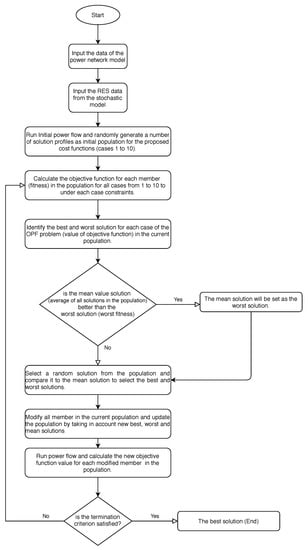
Figure 1. Flowchart of the proposed GROM to solve the OPF problem.

In general, numerical and conventional optimization methods are obtained decision variables by finding or randomly searching for a point at which the derivative is zero. However, implementation of these methods for energy and OPF problems are complicated with highly computational costs due to the non-convex, nonlinear and constrained nature of OPF problems for RES networks. Therefore, an optimization approach based on golden ratio algorithm is designed to improve the optimization performance in terms power network efficiency, energy and cost saving, gas emission reduction, convergence rate and computational cost. The main idea of GROM is to create an optimization solver based on a growth pattern in nature such as plants [22]. This pattern was discovered by Fibonacci, and he called it the golden ratio. This ratio determines the growth angle of the model and helps to achieve the optimal solution [22].

In this work, a GROM is developed to optimize the OPF for a power network connected to a wind and solar power generations and it outlined in Figure 1. Firstly, we create a number of random operation solutions for the OPF problem, such as population initialization, and calculate the mean value of the population. The next step in this phase is to compare fitness of the mean value solution to the worst solution. The fitness of each optimal operation profile is evaluated by using the cost objective functions for cases 1 to 10, as described in Section 2. In case the mean operation solution has a better fitness value compared to the worst operation solution, we replace the worst solution with the mean solution. This process aims to enhance the optimization speed to achieve convergence. Then, to determine the direction and the new solution movement, a random solution vector is selected for each solution in the population. In order to specify the direction of the new solution, the selected and the random solution vectors were compared to the mean solution vector. The random solution provides the ability of searching the whole space of the OPF problem and create a random movement towards the new solution. To determine the movement size and direction for obtained solution vector, Fibonacci’s formula (golden ratio) are used as in [22]. In this work, the best solution which has the best fitness value (minimum objective function value) is selected as the main solution vector. In the GROM algorithm, the solutions should be updated toward the best solution of the population under the RES network model constraints [22]. Finally, the proposed GROM method is a simple and free from any parameter tuning, which help to minimise the computational cost and convergence rate. In order to verify how the parameters of GROM has been selected, Section 3.3.1 present a statistical analysis for the GROM model and other meta-heuristic optimization strategies. The optimization parameters have been tested over a range of values, as presented in Section 3.3.1 and best solution was selected to obtain the results in this paper. The results and comparison shown in the following section present the performance of the proposed GROM method.

3. Results and Discussions

In this section, the results of the GROM algorithm are presented over ten cases of objective functions, as discussed in Section 2 in this paper. The GROM algorithm is compared to six metaheuristics optimization algorithms in this work, namely: Chaotic Gravitational Search Algorithm (CGSA)-1 [39], MPSO [38], CGSA2 [39], SDO [40], TLBO [41] and CGWO [42]. First, the optimization algorithms result for single objective functions are discussed; then the algorithms are tested over multi-objective functions cases. Throughout this subsection, we will compare the optimization algorithms performance for a specific power network model using the following configurations:

• Scenario 1: IEEE 30-bus without renewable energy sources.
  An IEEE 30-bus of six thermal power generating units is used as reference power network model in this paper [47,48,49], as described in Table 3 and Figure 2.
  Table 3. The general specifications of the IEEE 30-bus system.

  Characteristics	Values [47,48,49]
  Branches	41
  Number of buses	30
  Generators	6 (Buses:1, 2, 5, 8, 11 and 13)
  Swing bus	Bus 1
  Generator voltage limits	0.95–1.1 p.u
  Load voltage limits	0.95–1.05 p.u
  Setting of tap changer in transformer	0.9–1.1 p.u
  Transformer with tap ration	4 (Buses: 11, 12, 15 and 36)
  Voltage Automatic Regulator	0–5 p.u
  Shunt VAR compensation	9 Buses: 10, 12, 15, 17, 20, 21, 23, 24 and 29
  Real demand	2.834 p.u
  Reactive demand	1.262 p.u
  Load	100 MVA
  Control variables	24

  

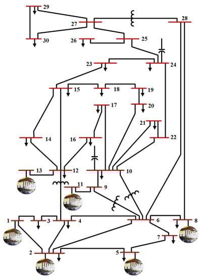  Figure 2. Scenario 1: IEEE 30-bus system.
• Scenario 2: IEEE 30-bus Modified (1).
  An IEEE 30-bus Modified (1) is presented to investigate the impact of adding RES with stochastic power generation behavior to the reference power network, as seen in Figure A1. Here, the IEEE 30-bus system modified by replacing the thermal power generators at buses 5, 11, and 13 with solar PV at buses 5 and 13 as well as wind generator at bus 11. Furthermore, two new renewable generators (solar PV and wind generator) have been added at bus 24 and 30, respectively. The IEEE 30-bus Modified (1) specifications is described in Table A1. The general specifications and data for wind and solar system which connected to the IEEE 30-bus Modified (1) are presented in Table A2 and Table A3, respectively.
• Scenario 3: IEEE 30-bus Modified (2)
  An IEEE 30-bus Modified (2) is simulated to show the optimization performance over different RES location scenarios, as presented in Figure A2. The IEEE 30-bus system has been modified in this case by adding solar generator at buses 5 and 13, and wind generator at bus 11 instead of the old thermal power generators. In addition, a new solar PV and wind generators has been located at buses 17 and 28, respectively. Table A6 presents the IEEE 30-bus Modified (2) specifications. The general specifications and data for wind and solar system which connected to the IEEE 30-bus Modified (2) are presented in Table A4 and Table A5, respectively.
  For scenario (2) and scenario (3), the cases (3, 5, 7, 8, 9, and 10) in Section 2.1 will be modified to involve the effect of the presence of wind and solar sources by adding the total cost of wind power generations $C_w^T$ and the total cost of solar power generations $C_S^T$ to their equations.
  The IEEE 30-bus, IEEE 30-bus Modified (1) and IEEE 30-bus Modified (2) systems are used to address OPF problem then solve them by GROM algorithm and other optimizations algorithms over 10 cases, as summarized in Table 4. The simulation models have been implemented on 2.8-GHz i7 PC with 16 GB of RAM using using MATLAB 2016 and the maximum number of iterations is set to 100 for the GROM model as in [22].
  Table 4. Summary of case studies.

  Name	Objective Function	Test Systems
  case 1	Real power loss minimization	All scenarios
  case 2	Emission index minimization	All scenarios
  case 3	Quadratic fuel cost with valve point loading minimization	All scenarios
  case 4	Enhancement of the voltage stability	All scenarios
  case 5	Basic fuel cost minimization	All scenarios
  case 6	Voltage deviation minimization	All scenarios
  case 7	Fuel cost minimization and voltage stability enhancement	All scenarios
  case 8	Fuel cost and voltage deviation minimization	All scenarios
  case 9	Minimization of basic fuel cost and active power loss	All scenarios
  case 10	Minimization of basic fuel cost, emission index, voltage deviation, and real power losses	All scenarios

3.1. Single-Objective OPF Problem Test Results

Table 4 presents ten cases for OPF problems, where the first six cases deal with solving single objective problems. Firstly, the optimization algorithms are tested by using IEEE 30-bus system without RES. Then, each case of objective function has been evaluated over the three power network models: IEEE 30-bus, IEEE 30-bus Modified (1), IEEE 30-bus Modified (2).

3.1.1. IEEE 30-Bus System without RES

In this subsection, the GROM is used to solve the single objective function considering the real power loss, gas emission, generation cost, voltage stability and deviation, as presented in Table 5, Figure 3, Figure 4 and Figure 5. Table 5 presents the results of the GROM algorithm and other optimization algorithms for IEEE 30-bus. The results of GROM algorithm are compared to the CGSA1 [39], MPSO [38], CGSA2 [39], SDO [40], TLBO [41] and CGWO [42]. Table 5 shows the GROM algorithm outperforms other optimization methods, where the objective function value solving by GROM algorithm was less than all other optimization methods. For example, the objective function of case 1 for GROM was 3.14394 MW compared to 4.02199 MW and 3.62014 MW for CGSA1 and SDO algorithms respectively. Figure 3 presents the convergence curves of the proposed GROM and other optimization algorithms over six cases (single objective functions). The GROM solver has smooth convergence curve over all single objective functions, cases 1 to 6, compared to other methods. The other optimization algorithms showed a volatile behavior, where the convergence curve change from one case to another. The proposed GROM achieves the optimal solution with oscillations behavior and speedy convergence rate compared to other methods. In addition, the proposed GROM model achieve the optimal solution without violate the constraints such as voltage. Figure 4 and Figure 5 show that the GROM maintains the voltages and transmission line loading magnitudes within the limits over all cases.

Table 5. Results of the GROM algorithm and other optimization algorithms for the single-objective OPF for IEEE 30-bus system.

Case #	Objective Functions	CGSA1	CGSA2	GROM	SDO	MPSO	TLBO	CGWO
case 1	VD (p.u.)	0.70714	0.66033	0.71999	0.42466	0.76014	0.91679	0.45222
	FC (USD/h)	872.15567	862.70849	973.92220	937.68429	974.61528	973.81103	882.43800
	Lindex (p.u.)	0.13921	0.14057	0.14115	0.14983	0.14049	0.13807	0.15171
	Ploss (MW)	4.02199	4.56792	3.14395	3.62014	3.63387	3.30616	3.81476
	E (ton/h)	0.24129	0.25443	0.20728	0.20859	0.20731	0.20727	0.23832
	FC_vlv (USD/h)	938.22643	919.87682	1034.34424	1010.80552	1035.17883	1034.19025	948.79631
	f	4.02199	4.56792	3.14395	3.62014	3.63387	3.30616	3.81476
case 2	VD (p.u.)	0.30358	0.26136	0.71076	0.43636	0.47812	0.85723	0.34289
	FC (USD/h)	893.51907	904.71244	950.66290	937.92776	952.22920	950.84888	922.64268
	Lindex (p.u.)	0.15305	0.14919	0.14162	0.14172	0.14156	0.13870	0.14467
	Ploss (MW)	4.75735	4.86732	3.27565	4.13267	3.72861	3.24525	4.35506
	E (ton/h)	0.21014	0.21175	0.20484	0.20833	0.20498	0.20954	0.21590
	FC_vlv (USD/h)	966.67831	979.85891	1022.44605	1011.69196	1024.07955	1022.49926	996.83934
	f	0.21014	0.21175	0.20484	0.20833	0.20498	0.20954	0.21590
case 3	VD (p.u.)	0.74420	0.76043	0.54279	0.48761	0.82239	0.87906	0.21039
	FC (USD/h)	841.77721	841.43518	843.27611	845.83292	847.23728	843.45433	845.28956
	Lindex (p.u.)	0.13925	0.13894	0.14295	0.14344	0.14049	0.13830	0.14515
	Ploss (MW)	6.92302	6.91765	7.59137	7.78547	8.40996	7.55869	7.85219
	E (ton/h)	0.28202	0.28216	0.29454	0.29500	0.29544	0.29499	0.28347
	FC_vlv (USD/h)	888.61875	888.26826	878.81470	881.40390	882.00880	880.27966	890.33615
	f	888.61875	888.26826	878.81470	881.40390	882.00880	880.27966	890.33615
case 4	VD (p.u.)	0.52152	0.69797	0.76302	0.61286	0.77076	0.80003	0.41698
	FC (USD/h)	847.68847	857.20269	865.24315	878.07633	965.79266	842.18148	868.30374
	Lindex (p.u.)	0.13961	0.13843	0.13763	0.13833	0.13831	0.13780	0.13955
	Ploss (MW)	7.35211	6.53377	5.83031	6.16208	4.06270	7.63168	6.21642
	E (ton/h)	0.27847	0.27138	0.25335	0.25025	0.20972	0.28532	0.25784
	FC_vlv (USD/h)	893.86133	904.43303	923.05396	935.29245	1028.15088	884.27804	922.55697
	f	0.13961	0.13843	0.13763	0.13833	0.13831	0.13780	0.13955
case 5	VD (p.u.)	0.65735	0.81414	0.58429	0.37576	0.55693	0.87181	0.34863
	FC (USD/h)	842.67436	843.95553	837.59102	842.46418	842.54683	840.67292	847.02139
	Lindex (p.u.)	0.14093	0.13784	0.14318	0.15094	0.14409	0.13837	0.14615
	Ploss (MW)	7.31461	6.64161	7.00648	7.28322	7.46838	6.96988	7.15725
	E (ton/h)	0.28127	0.27959	0.28517	0.28468	0.28550	0.28551	0.28116
	FC_vlv (USD/h)	890.30092	892.37037	882.09685	884.12811	883.49168	881.53172	891.18054
	f	842.67436	843.95553	837.59102	842.46418	842.54683	840.67292	847.02139
case 6	VD (p.u.)	0.12821	0.13251	0.09950	0.13142	0.12680	0.12699	0.13714
	FC (USD/h)	851.54629	855.78998	908.24429	861.13868	950.00101	868.79324	854.19234
	Lindex (p.u.)	0.14838	0.14789	0.14810	0.14825	0.14658	0.14753	0.14635
	Ploss (MW)	7.07079	6.94105	5.22157	6.68247	4.58518	5.90128	7.03471
	E (ton/h)	0.27491	0.27301	0.23516	0.25901	0.21851	0.25806	0.27187
	FC_vlv (USD/h)	899.37305	903.61970	970.73639	915.38549	1014.22195	922.65231	901.26322
	f	0.12821	0.13251	0.09950	0.13142	0.12680	0.12699	0.13714

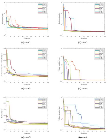
Figure 3. Convergence curves for single-objective optimal power flow.

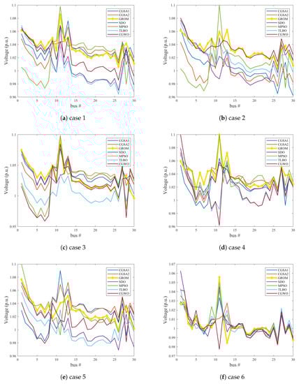
Figure 4. Voltage profile for single-objective optimal power flow.

Figure 5. Loading profile for single-objective optimal power flow.

3.1.2. IEEE 30-Bus System with RES

In this subsection, the GROM is applied to solve the OPF problem over six cases incorporating RES (IEEE 30-bus Modified (1) and IEEE 30-bus Modified (2)). In addition, the proposed GROM results will be compared to other six metaheuristics optimization algorithms in Section 3.3.

• Case 1: Real power loss minimization
  In this case the GROM is applied to solve the OPF problem for a power network with and without RES considering only the real power loss. By adding the wind and PV model as a negative load to the IEEE 30-bus system (Modified 1 and 2), the total load demand and power losses are reduced. Figure 6 shows the power loss and loading prolife for the three system cases: IEEE 30-bus system, IEEE 30-bus Modified (1) and IEEE 30-bus Modified (2). The power loss in IEEE 30-bus Modified (1) and IEEE 30-bus Modified (2) was reduced by 37.85% and 22.9%, respectively compared to IEEE 30-bus system without RES. The GROM results for case 1 and all other cases will be presented are compared to other proposed optimization methods in Section 3.3.
  

  Figure 6. Loss and Loading Profiles for case 1 for IEEE 30-bus system, IEEE 30-bus Modified (1) and IEEE 30-bus Modified (2).
• Case 2: Emission index minimization
  In this case, the environmental impact in the power networks is considered and analysed. A gas emission analysis has been carried out for the three proposed IEEE systems to show the environmental benefits of optimally control the power generations. Figure 7 presents the emission index for GROM model in all network scenarios with or without RES. The GROM can achieve an emission index savings of around 55.54% for IEEE 30-bus model with RES (Modified (1) and (2)) compared to IEEE 30-bus model without RES. In IEEE 30-bus model with RES, the wind and PV system allows a reduction in the number of thermal power generation to meet the required load demand.
  

  Figure 7. Emission index (ton/hr) for case 2 IEEE 30-bus system, IEEE 30-bus Modified (1) and IEEE 30-bus Modified (2).
• Case 3: Minimization of the cost of Fuel with value point effect of thermal power, wind, and solar PV generating units
  In case 3, the GROM algorithm is designed to achieve a substantial saving in the fuel and power generation costs. The economic power generation is considered and analysed in this section. The analysis of power generations cost with valve point effect of thermal power has been presented to show the commercial benefits of the optimality control IEEE power system with and without RES. In Figure 8, the total power generations cost has been computed and presented. The GROM algorithm can reduce the power generations cost in IEEE 30-bus Modified (1) and IEEE 30-bus Modified (2) by around 8.69% and 6.68%, respectively, compared to IEEE 30-bus without RES. The power generation cost saving results show that the RES networks improved the economic performance compared to power network without RES.
  

  Figure 8. Fuel cost with valve point effect (USD/hr) for case 3 for IEEE 30-bus system, IEEE 30-bus Modified (1) and IEEE 30-bus Modified (2).
• Case 4: Minimization of voltage stability index
  In this case, the voltage stability index was optimized by using GROM algorithm for IEEE 30- bus network with and without RES. The power quality related to voltage stability is considered in this section. The analysis of voltage stability has been carried out to present the power quality benefits of optimality control IEEE power system with and without RES. Figure 9 shows that the GROM can improve the voltage stability index by 52% and 50% for IEEE 30-bus Modified (1) and IEEE 30-bus Modified (2), respectively, compared to IEEE 30-bus system without RES.
  

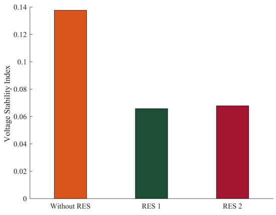  Figure 9. Voltage Stability Index (p.u.) for IEEE 30-bus system, IEEE 30-bus Modified (1) and IEEE 30-bus Modified (2).
• Case 5: Minimization of the cost of Fuel of thermal power, wind, and solar PV generating units
  The economic power generation based on the basic cost function is analysed in this section, as seen in Figure 10. The basic fuel cost, as discussed in Section 2, of thermal power generators, wind, and solar generating have optimized for power networks with and without RES. The GROM algorithm can reduce the total generation cost for IEEE 30-bus Modified (1) and (2) by 7.87% and 8.93%, respectively, compared to IEEE 30-bus without RES; in addition, the power generation contribution from renewable energy was 40% and 39%, respectively.
  

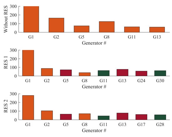  Figure 10. Fuel cost (USD/hr) for IEEE 30-bus system, IEEE 30-bus Modified (1) and IEEE 30-bus Modified (2).
• Case 6: Voltage deviation minimization
  In this section, a cost function for voltage deviation has been used to show the impact of optimally control on power networks. Figure 11 presents the voltage profile for IEEE 30-bus system, IEEE 30-bus Modified (1) and IEEE 30-bus Modified (2). As seen in Figure 11, the GROM algorithm can improve the voltage profile behavior by reducing the voltage deviation. The voltage deviation was reduced by 23.9% and 12.1% for IEEE 30-bus Modified (1) and IEEE 30-bus Modified (2), respectively, compared to IEEE 30-bus system without RES.
  

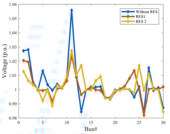  Figure 11. Voltage deviation (p.u.) IEEE 30-bus system, IEEE 30-bus Modified (1) and IEEE 30-bus Modified (2).

3.2. Multi-Objective OPF Problem Test Results

In recent years, the planning and operation of power networks with high penetration of RES is becoming more significant due to the fuel cost and environment challenges. In general, the Optimization Power Flow (OPF) problem of the different thermal and renewable energy sources is a multi-objective function problem because it consider many problem terms such as economical (power generation costs), technical (voltage stability and deviation) and environmental (gas emission). In multi-objective function, the main aim is to simultaneously optimize more than one objective function based on the trade-offs between two or more conflicting single optimization objectives. For example, maximizing cost savings while minimizing power loss and gas emissions in a power network. The solution multi objective functions are generally associated with a high computational cost due to number of variables, constraints and design options. This section presents four cases of multi-objective OPF problems, the GROM is used to solve the multi-objective function considering the real power losses, gas emission, generation cost, voltage stability and deviation. Firstly, the GROM is tested by using IEEE 30-bus system without RES. Then, each case of objective function has been evaluated for the three power network models: IEEE 30-bus, IEEE 30-bus Modified (1), IEEE 30-bus Modified (2). The following section, Section 3.3, will compare and evaluate all proposed optimization methods for different power network models.

3.2.1. IEEE 30-Bus System without RES

In this subsection, the GROM is used to solve multi-objective OPF problem (case 7 to case 10) considering the real power losses, gas emission, generation cost, voltage stability and deviation, as presented in Table 4. The results of GROM algorithm are compared to other proposed optimization methods. Table 6 shows the GROM algorithm outperforms other optimization methods for IEEE 30-bus system, where the multi-objective function value solving by GROM algorithm was less than all other optimization methods. For example, the objective function of case 7 for GROM was 851.23146 USD/h compared to 854.04331 USD/h and 857.33158 USD/h for TLBO [41] and CGWO [42] algorithms, respectively. Figure A3 presents the convergence curves of the proposed GROM and other optimization algorithms over four multi-objective cases. The GROM solver has smooth convergence curve over all cases and achieve the optimal solution without oscillations and a speedy convergence rate compared to other methods. The proposed GROM model achieves the optimal solution without violating the constraints, such as voltage, as presented in Figure A4 and Figure A5. The results show that the GROM maintains the voltages and transmission line loading magnitudes within the limits over all cases.

Table 6. Results of the GROM algorithm and other optimization algorithms for the multi-objective OPF for IEEE 30-bus system.

Case #	Objective Functions	CGSA1	CGSA2	GROM	SDO	MPSO	TLBO	CGWO
case 7	VD (p.u.)	0.71956	0.81489	0.86632	0.43614	0.45958	0.77051	0.27146
	FC (USD/h)	842.34211	843.56498	837.44271	838.93332	840.32568	840.22379	843.02072
	Lindex (p.u.)	0.13874	0.13754	0.13789	0.14714	0.14368	0.13820	0.14311
	Ploss (MW)	7.13032	6.72718	7.01754	7.16570	7.68514	7.11366	7.67649
	E (ton/h)	0.28088	0.27965	0.28556	0.28438	0.28570	0.28491	0.29099
	FC_vlv (USD/h)	890.25298	891.98861	881.63306	884.05295	884.44747	882.83589	883.69004
	f	856.21598	857.31884	851.23146	853.64758	854.69399	854.04331	857.33158
case 8	VD (p.u.)	0.14185	0.13693	0.14047	0.16387	0.16498	0.11196	0.20062
	FC (USD/h)	845.70694	850.00253	840.25665	840.62723	846.76444	843.16209	846.84117
	Lindex (p.u.)	0.14816	0.14788	0.14795	0.14730	0.14672	0.14838	0.14738
	Ploss (MW)	7.21634	7.01876	7.48091	7.62987	8.79324	7.58708	7.86412
	E (ton/h)	0.27951	0.27932	0.28370	0.28525	0.28767	0.28371	0.28564
	FC_vlv (USD/h)	894.33354	898.18813	886.12943	885.16084	889.46656	886.40801	889.31964
	f	859.89232	863.69596	854.30414	857.01426	863.26244	854.35856	866.90351
case 9	VD (p.u.)	0.85180	0.81605	0.93868	0.83308	0.89428	0.92644	0.50486
	FC (USD/h)	870.88439	855.92392	901.66376	894.05610	900.12790	901.38918	896.53237
	Lindex (p.u.)	0.13870	0.13923	0.13814	0.13913	0.13735	0.13779	0.14444
	Ploss (MW)	5.12427	6.01478	3.92221	4.15095	4.09287	3.98993	4.77420
	E (ton/h)	0.24102	0.26299	0.22229	0.22631	0.22344	0.22257	0.22338
	FC_vlv (USD/h)	937.37032	907.60089	976.76381	967.69190	973.03795	973.72474	971.58135
	f	1075.85533	1096.51494	1058.55236	1060.09426	1063.84270	1060.98618	1087.50030
case 10	VD (p.u.)	0.31594	0.22964	0.29715	0.29599	0.24263	0.22534	0.30006
	FC (USD/h)	858.18018	865.49723	861.40594	873.46881	865.78551	866.33761	862.24483
	Lindex (p.u.)	0.14591	0.14746	0.14696	0.14638	0.14809	0.14747	0.14697
	Ploss (MW)	5.75921	5.76015	5.31786	5.07336	5.41304	5.37209	6.09696
	E (ton/h)	0.25409	0.24952	0.24968	0.24182	0.24795	0.24776	0.26427
	FC_vlv (USD/h)	916.24654	926.00808	922.20928	936.71876	925.34475	925.32501	909.59909
	f	996.34524	1001.78360	989.38294	995.89322	994.67865	993.96323	1007.70037

3.2.2. IEEE 30-Bus System with RES

In order to evaluate the impact of adding RES to power network on optimization performance, the GROM is applied to solve the OPF problem over four cases incorporating RES (IEEE 30-bus Modified (1) and IEEE 30-bus Modified (2)). The proposed GROM results will be compared to six metaheuristics optimization algorithms in the following section, Section 3.3.

• Case 7: Minimization of the cost of fuel of thermal power, wind, and solar PV generating units and voltage stability index.
  In this case, energy generation cost and voltage stability index was minimized as a multi-objective function for a power network with and without RES, as presented in Figure 12. By adding the wind and PV model to the IEEE 30-bus system (Modified 1 and 2) and using the GROM to solve the multi-objective OPF problem in this section, the total power generation cost is reduced. Figure 12a shows the total generations cost for the three power system cases: IEEE 30-bus system, IEEE 30-bus Modified (1) and IEEE 30-bus Modified (2). The total generations cost in IEEE 30-bus Modified (1) and IEEE 30-bus Modified (2) was reduced by 5.16% and 8%, respectively, compared to IEEE 30-bus system without RES. The generations cost reduction is basically coming from the increase in RES contribution power network. The wind and solar power generations were increased by 36% and 39%, respectively. In addition, the voltage stability index, as shown in Figure 12b, for IEEE 30-bus Modified (1) and IEEE 30-bus Modified (2) systems were reduced by 45.3% and 44.1%, respectively, as compared to IEEE 30-bus system.
  

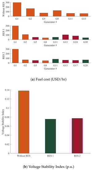  Figure 12. Fuel cost and Voltage Stability Index for case 7 for IEEE 30-bus system, IEEE 30-bus Modified (1) and IEEE 30-bus Modified (2).
• Case 8: Minimization of the cost of Fuel of thermal power, wind, and solar PV generating units and voltage deviation.
  The economic power generation and voltage deviation terms are analysed in this section, as seen in Figure 13. A multi-objective cost function for voltage deviation and power generations cost has been used to show the impact of optimally power control on these terms. The GROM algorithm can reduce the total generations cost for IEEE 30-bus Modified (1) and (2) by 4.3% and 7.38%, respectively, compared to IEEE 30-bus without RES, as shown in Figure 13a. The voltage profiles, as presented in Figure 13b, for IEEE 30-bus system, IEEE 30-bus Modified (1) and IEEE 30-bus Modified (2) have been improved by reducing the voltage deviation. The voltage deviation was improved by 0.26% and 22.76% for IEEE 30-bus Modified (1) and IEEE 30-bus Modified (2), respectively, compared to IEEE 30-bus system without RES.
  

  Figure 13. Fuel cost and Voltage deviation for case 8 for IEEE 30-bus system, IEEE 30-bus Modified (1) and IEEE 30-bus Modified (2).
• Case 9: Minimization of power loss and total power generations cost.
  In this case the GROM is applied to solve multi-objective OPF problem for a power network with and without RES considering only the real power loss and the total power generations cost. Figure 14a shows that the total power generation cost in IEEE 30-bus Modified (1) and IEEE 30-bus Modified (2) was reduced by 10.87% and 7.56%, respectively, compared to IEEE 30-bus system without RES. In addition, the power loss in IEEE 30-bus Modified (1) and IEEE 30-bus Modified (2) was reduced by 23% and 19%, respectively, compared to IEEE 30-bus system without RES, as shown in Figure 14b.
  

  Figure 14. Fuel cost and Real power loss for case 9 for IEEE 30-bus system, IEEE 30-bus Modified (1) and IEEE 30-bus Modified (2).
• Case 10: Minimization of the total power generations cost, voltage deviation, real power loss, and emission index.
  In order to evaluate the GROM algorithm performance with highly complex multi-objective function, case 10 is presented in this section. Here, the multi-objective function describes four terms: the total power generations cost, voltage deviation, real power loss, and gas emission index. In this section, the GROM is applied to solve the multi-objective OPF problem for power network incorporating RES (IEEE 30-bus Modified (1) and IEEE 30-bus Modified (2)), as shown in Figure 15. Firstly, the total generation cost was reduced by 6% and 6.9% for RES networks (IEEE 30-bus Modified (1) and IEEE 30-bus Modified (2)), respectively, compared to IEEE 30-bus without RES, as shown in Figure 15a. Similarly, the power loss reduction and voltage deviation was also improved by 23.6% and 40.8% for IEEE 30-bus Modified (1), respectively, as presented in Figure 15b,c. Finally, the gas emission index was reduced by 56% and 57% for RES networks (IEEE 30-bus Modified (1) and IEEE 30-bus Modified (2)), respectively, compared to IEEE 30-bus without RES, as shown in Figure 15d.
  

  Figure 15. The total power generation cost, real power loss, voltage deviation, and Emission index IEEE 30-bus system, IEEE 30-bus Modified (1) and IEEE 30-bus Modified (2).

3.3. Discussion and Comparison

This section compares the performance of proposed GROM algorithms in this paper and other optimization methods (CGSA1 [39], MPSO [38],CGSA2 [39], SDO [40], TLBO [41] and CGWO [42]). The convergence rate of the GROM is computed based on number of iterations in accordance with single and multi-objective OPF problems. The convergence rate comparison is presented in Section 3.1 and Section 3.2 for IEEE-30 bus systems over ten cases. Figure 3 and Figure A3 showed that the proposed GROM algorithm achived the optimal solutions within a less number of iterations which will reduce the computational cost. Therefore, the GROM algorithm shows a higher ability to solve complex OPF problem with and without RES. Table 7 shows the GROM algorithm performance compared to CGSA1 [39], MPSO [38],CGSA2 [39], SDO [40], TLBO [41] and CGWO [42]. The results show that the GROM algorithm improved the objective function performance in each case of the ten cases compared to other optimization methods. For example, the power loss reduction (case 1) has been improved by 21.8% and 17.5% compared to CGSA and CGWO, respectively.

Table 7. Improvement of objective functions of GROM over other techniques.

	Case 1	Case 2	Case 3	Case 4	Case 5	Case 6	Case 7	Case 8	Case 9	Case 10
CGSA1	21.831%	2.526%	1.103%	1.418%	0.603%	22.392%	0.582%	0.650%	1.608%	0.699%
CGSA2	31.173%	3.266%	1.064%	0.577%	0.754%	24.910%	0.710%	1.087%	3.462%	1.238%
SDO	13.154%	1.679%	0.294%	0.506%	0.578%	24.284%	0.283%	0.316%	0.145%	0.654%
MPSO	13.482%	0.069%	0.362%	0.496%	0.588%	21.528%	0.405%	1.038%	0.497%	0.532%
TLBO	4.906%	2.244%	0.166%	0.123%	0.367%	21.642%	0.329%	0.006%	0.229%	0.461%
CGWO	17.584%	5.124%	1.294%	1.375%	1.113%	27.444%	0.712%	1.453%	2.662%	1.818%

Similarly, the GROM algorithm is tested with and without connecting RES (wind and solar power systems) to IEEE 30-bus network systems. In addition, the wind and solar system have been located in different location (IEEE 30-bus Modified (1) and IEEE 30-bus Modified (2)) to evaluate the impact of RES location on the GROM and other optimization methods, as shown in Figure 16. Table 8 and Table 9 and Figure 16 present the GROM algorithm performance for IEEE 30-bus Modified (1) and IEEE 30-bus Modified (2)) with compared to IEEE 30-bus without RES. The results show that the GROM algorithm improved the objective function performance for the both RES power network simulations over the ten proposed cases. For example, Figure 16e shows that the voltage stability (case 4) has been improved by 52.2% and 50.7% for IEEE 30-bus Modified (1) and IEEE 30-bus Modified (2), respectively, compared to IEEE 30-bus without RES. The GROM simulation results for all objective function cases and power network scenarios have been presented in Table A7, Table A8, Table A9, Table A10, Table A11, Table A12, as Appendix A for this paper

Figure 16. Overall comparisons for real power loss, total cost, total emission, voltage deviation, and voltage stability index IEEE 30-bus system, IEEE 30-bus Modified (1) and IEEE 30-bus Modified (2).

Table 8. Improvement of objective functions for GROM between scenario 1 and scenario 2.

Case 1	Case 2	Case 3	Case 4	Case 5	Case 6	Case 7	Case 8	Case 9	Case 10
37.856%	55.542%	10.691%	52.202%	7.866%	23.966%	5.806%	4.251%	12.687%	8.558%

Table 9. Improvement of objective functions for GROM between scenario 1 and scenario 3.

Case 1	Case 2	Case 3	Case 4	Case 5	Case 6	Case 7	Case 8	Case 9	Case 10
22.918%	55.544%	9.846%	50.710%	8.932%	12.095%	8.580%	6.888%	9.283%	9.243%

3.3.1. Analysis of GROM and Other Meta-Heuristics Optimization Strategies

The previous sections introduced the GROM method as a more suitable optimization method compared to other meta-heuristics methods. This section will further elaborate and provide evidence on the performance of GROM method and identify the parameters of each proposed method. The proposed optimization methods were applied to solve single objective OPF problem considering the real power loss (case 1) and multi objective function considering the total power generations cost, voltage deviation, real power loss, and emission index (case 10). In this section, the proposed optimization methods were tested to investigate the superiority of the GROM method compared to other proposed methods. Table 10 and Table 11 presents the statistical analysis for the objective function value over 20 runs of simulations for case 1 and case 10. Analysis of the objective function value is shown in Table 10 and Table 11 to present various statistics of objective value including the minimum, maximum, median and standard deviation values. Table 10 and Table 11 shows that the standard deviation for the GROM method for case 1 and case 10 was the minimum value compared to other optimization methods with values equal to 0.0130 and 0.3787, respectively. The proposed GROM outperform other metaheuristics methods in solving the single and multi-objective function without any violation to the constraints. For example, the maximum objective function value for GROM method was 3.141349 compared to 6.078505 for CGSA2.

Table 10. Statistical analysis for case 1.

	Min	Max	Median	Standard Devaition
CGSA1	4.767784	5.77408	5.303694	0.2887
CGSA2	5.126046	6.078505	5.500868	0.2809
GROM	3.086593	3.141349	3.092469	0.0130
SDO	3.459937	3.98322	3.639853	0.1424
MPSO	3.101988	4.640072	3.414303	0.3657
TLBO	3.093546	3.175361	3.119197	0.0206
CGWO	3.098536	3.491199	3.297122	0.1221

Table 11. Statistical analysis for case 10.

	Min	Max	Median	Standard Devaition
CGSA1	993.5015	1004.872	996.5863	3.0276
CGSA2	994.9444	1002.978	1000.033	2.0206
GROM	989.1602	990.6765	989.7054	0.3787
SDO	991.742	994.6512	993.0029	0.8192
MPSO	990.0802	1009.702	991.5875	6.1010
TLBO	989.1987	992.033	989.8508	0.7791
CGWO	989.3301	993.7202	990.8954	1.0713

In complex OPF problems and multi-objective functions, the optimization solvers aim to find the best compromise solution. However, there is no general superior optimization approach to solve all multi-objective function problems. Generally, developing a specific optimization method will rely on number factors such as the OPF problem complexity, types and number of constraints, the available information in the model and the type of simulation and software packages. Furthermore, each optimization solver has drawbacks and advantages some of these solvers can be only used for specific optimization problems. This section aims to verify how the parameters of each solver has been selected by using the previous studies information and comparing the results of the non-dominated and the best compromise solutions for each optimization solver. Table 12 the main parameters of each of the proposed of optimization algorithms in this paper. The optimization parameters have been tested over a range of values, as presented in Table 12 and best solution was selected to obtain the results in this paper.

Table 12. Parameters and testing ranges of optimization algorithms.

Algorithm	Parameters	Values	Testing Range and Notes
TLBO [41]	Teaching factor (TF) Maximum Number of Iterations Population Size Random number (r)	Selected randomly between 1 and 2 100 50 A uniformly distributed random number (0, 1)	[50, 100, 200] [25, 50, 100]
MPSO [38]	Inertia coefficient (w) Number of search agents Maximum number of iteration acceleration coefficient (c1, c2)	linearly reducing from 0. 9 to 0.4 50 100 c1 = 1 and c2 = 2	[50, 100, 200] [25, 50, 100]
	Udapting factors (C1, C2)	Descriped in [38]	Depending on: 1-the maximum number of iterations 2-the current iteration 3- random number ranges between 0 and 1
SDO [39]	Weights α and β	Descriped in [39]	Depending on: 1-the maximum number of iteration 2-the current iteration
	The size of markets The maximum number of iterations Random number (r)	50 100 ranged from 0 and 1	[50, 100, 200] [25, 50, 100]
CGWO [42]	Random vectors (r1, r2) Number of search agents Maximum number of iteration chaotic function variables (a, b) controlling parameter (a)	ranged from 0 and 1 50 100 a = 0.5 and b = 0.2 decreasing linearly from 2 to 0	[50, 100, 200] [25, 50, 100]
CGSA1 [39]	initial gravitational constant (G0) the descending coefficient (α) Number of search agents The maximum number of iterations choatic map	100 10 50 100 defined by chebyshev	[50, 100, 200] [25, 50, 100]
CGSA2 [39]	initial gravitational constant (G0) Number of search agents The maximum number of iterations the descending coefficient (a) choatic map	100 50 100 10 defined by circle	[50, 100, 200] [25, 50, 100]
GROM [22]	Golden ratio (ϕ) Number of search agents Maximum number of iteration	1.618 50 100	[50, 100, 200] [25, 50, 100]

3.3.2. OPF for Largescale System

This section aims to check and test the scalability of the proposed GROM for a large-scale power network system (IEEE 118-bus) without RES, similar to scenario 1. The data about generators, buses, and transmission lines are given in [49]. The permissible ranges of transformer tap settings and generator bus voltages are within [0.90, 1.10] and [0.95, 1.10], respectively [43], while the ratings of shunt compensators are within 0 and 25 MVAr [43]. The proposed metaheuristics optimization methods are applied to solve OPF problem considering the fuel cost of the thermal power generating units (Case 5). Table 13 shows that the proposed GROM outperform other metaheuristics methods in solving the OPF problem for in a large-scale system (case 5) without any violation to the constraints. For example, these results show that the fuel cost for GROM was reduced by 7.7% compared to MPSO and CGSA1. The objective function value for GROM method was the lowest value (135,861 USD/h) compared other methods such as SDO with (140,023 USD/h) and CGSA1 with (143,381 USD/h). In addition, the optimal solution obtained by GROM for IEEE 118-bus system is presented in Table 14.

Table 13. Results of the GROM and other optimization algorithms for large scale system (IEEE 118-bus system).

Objective Function	CGWO	GROM	SDO	MPSO	CGSA1	CGSA2	TLBO
FC (USD/h)	142,997	135,861	140,023	141,772	146,287	143,381	135,911

Table 14. Optimal solution obtained by GROM for IEEE 118-bus system.

Parameters	Range	Values	Parameters	Values	Parameters	Values
PG1	30–100	32.21186	VG1	0.95	QC5	0.950906
PG4	30–100	30	VG4	0.95	QC34	6.314366
PG6	30–100	30.04239	VG6	0.95	QC37	25
PG8	30–100	30.09265	VG8	0.950009897	QC44	25
PG10	165–550	311.3139	VG10	0.950003187	QC45	14.47493
PG12	55.5–185	61.43965	VG12	0.950003586	QC46	5.190185
PG15	30–100	30.2096	VG15	0.953660848	QC48	0.006565
PG18	30–100	30	VG18	0.950017838	QC74	3.810963
PG19	30–100	30	VG19	0.950095893	QC79	1.942429
PG24	30–100	30.59164	VG24	0.953394037	QC82	2.659867
PG25	96–320	135.8435	VG25	0.95621796	QC83	18.53097
PG26	124.2–414	223.4098	VG26	0.950713633	QC105	24.82019
PG27	30–100	30.13422	VG27	0.950069414	QC107	1.935545
PG31	32.1–107	32.10123	VG31	0.954585313	QC110	24.99855
PG32	30–100	30	VG32	0.950058989	TS8	0
PG34	30–100	30.18909	VG34	0.952406433	TS32	0.900319
PG36	30–100	30.30491	VG36	0.950089208	TS36	0.900039
PG40	30–100	30.06914	VG40	0.95185859	TS51	0.902047
PG42	30–100	30.07363	VG42	0.95	TS93	0.900013
PG46	35.7–119	35.7	VG46	0.950000035	TS95	0.901979
PG49	91.2–304	166.7628	VG49	0.95	TS102	0.900152
PG54	44.4–148	48.39637	VG54	0.950197974	TS107	0.90142
PG55	30–100	30.33253	VG55	0.950411434	TS127	0.90332
PG56	30–100	30.08466	VG56	0.95	PG69	372.5248
PG59	76.5–255	92.1767	VG59	0.950126059	FC	135861.6
PG61	78–260	129.9819	VG61	0.954125271
PG62	30–100	30.07884	VG62	0.950029822
PG65	147.3–491	302.9139	VG65	0.9500037
PG66	147.6–492	304.2236	VG66	0.950033728
PG70	30–100	30	VG70	0.950327527
PG72	30–100	30	VG72	0.95
PG73	30–100	30.20381	VG73	0.950007126
PG74	30–100	30	VG74	0.950003692
PG76	30–100	30.62061	VG76	0.95
PG77	30–100	30.04887	VG77	0.950010968
PG80	173.1–577	370.2427	VG80	0.950099868
PG85	30–100	31.42712	VG85	0.950001805
PG87	31.2–104	31.20093	VG87	0.951705271
PG89	212.1–707	387.9401	VG89	0.95
PG90	30–100	30.13136	VG90	0.95
PG91	30–100	30.26185	VG91	0.95
PG92	30–100	30.01491	VG92	0.950829199
PG99	30–100	30	VG99	0.950158643
PG100	105.6–352	168.2852	VG100	0.95
PG103	42–140	42.08391	VG103	0.95144805
PG104	30–100	30.65275	VG104	0.952230011
PG105	30–100	30.03129	VG105	0.950045069
PG107	30–100	33.67704	VG107	0.95
PG110	30–100	30.00487	VG110	0.95001117
PG111	40.8–136	40.94514	VG111	0.950369113
PG112	30–100	31.75673	VG112	0.950006161
PG113	30–100	30	VG113	0.950247127
PG116	30–100	30.49714	VG116	0.9500221

Figure 16 shows that the GROM solver has smooth convergence curve compared to other methods. The proposed GROM achieve the optimal solution with oscillations behaviour and speedy convergence rate compared to other methods even for large scale system. The comparisons result in Table 13 and Figure 17 showed that the GROM outperforms other methods for large scale similar to small scale systems and the objective function is similarly reduced as expected.

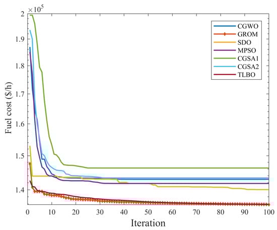
Figure 17. Convergence Curves for IEEE 118-bus system.

4. Conclusions

In this paper, a new proposed GROM method has been applied to single and multi-objective OPF problems for IEEE 30-bus system incorporating RES in different locations. The OPF problems have been presented by ten cases considering the total power generations cost, gas emission, power loss, voltage stability and voltage deviation. The OPF problem has been developed with a realistic model for the wind and solar systems, this model describes the stochastic nature of RES. The main goal of this work is providing a new optimization method able to overcome the drawbacks of the conventional optimization methods by developing a stochastic model for RES. The effectiveness GROM have been tested compered to six metaheuristics optimization algorithms, namely: CGSA1 [39], MPSO [38], CGSA2 [39], SDO [40], TLBO [41] and CGWO [42]. The comparisons’ results show that the GROM outperformed all other proposed optimization methods for power networks with or without RES. Different optimization techniques have been developed and used in this article to present and compare a sufficient number of new and efficient OPF problem solvers from which the decision maker and network operators can select the suitable solver solutions.The implementation of the proposed optimization methods in this paper is part of our future work. In addition, the impact of adding energy storage system to the power notwork is recommended.

References

- Shi, L.; Wang, C.; Yao, L.; Ni, Y.; Bazargan, M. Optimal power flow solution incorporating wind power. IEEE Syst. J. 2011, 6, 233–241. [Google Scholar] [CrossRef]
- Alasali, F.; Haben, S.; Holderbaum, W. Energy management systems for a network of electrified cranes with energy storage. Int. J. Electr. Power Energy Syst. 2019, 106, 210–222. [Google Scholar] [CrossRef]
- Roy, R.; Jadhav, H. Optimal power flow solution of power system incorporating stochastic wind power using Gbest guided artificial bee colony algorithm. Int. J. Electr. Power Energy Syst. 2015, 64, 562–578. [Google Scholar] [CrossRef]
- Biswas, P.P.; Suganthan, P.N.; Mallipeddi, R.; Amaratunga, G.A. Optimal reactive power dispatch with uncertainties in load demand and renewable energy sources adopting scenario-based approach. Appl. Soft Comput. 2019, 75, 616–632. [Google Scholar] [CrossRef]
- Biswas, P.P.; Suganthan, P.; Amaratunga, G.A. Optimal power flow solutions incorporating stochastic wind and solar power. Energy Convers. Manag. 2017, 148, 1194–1207. [Google Scholar] [CrossRef]
- Dommel, H.; Tinney, W. Optimal Power Flow solutions. IEEE Trans. Power Appar. Syst. 1968, PAS–87, 1866–1876. [Google Scholar] [CrossRef]
- Alasali, F.; Haben, S.; Holderbaum, W. Stochastic optimal energy management system for RTG cranes network using genetic algorithm and ensemble forecasts. J. Energy Storage 2019, 24, 100759. [Google Scholar] [CrossRef]
- Lin, W.M.; Huang, C.H.; Zhan, T.S. A hybrid current-power optimal power flow technique. IEEE Trans. Power Syst. 2008, 23, 177–185. [Google Scholar] [CrossRef]
- Glavitsch, H.; Spoerry, M. Quadratic loss formula for reactive dispatch. IEEE Trans. Power Appar. Syst. 1983, 102, 3850–3858. [Google Scholar] [CrossRef]
- Burchett, R.; Happ, H.; Wirgau, K. Large scale optimal power flow. IEEE Trans. Power Appar. Syst. 1982, 10, 3722–3732. [Google Scholar] [CrossRef]
- Shargh, S.; Mohammadi-Ivatloo, B.; Seyedi, H.; Abapour, M. Probabilistic multi-objective optimal power flow considering correlated wind power and load uncertainties. Renew. Energy 2016, 94, 10–21. [Google Scholar] [CrossRef]
- Lobato, E.; Rouco, L.; Navarrete, M.; Casanova, R.; Lopez, G. An LP-based optimal power flow for transmission losses and generator reactive margins minimization. In Proceedings of the 2001 IEEE Porto Power Tech Proceedings (Cat. No. 01EX502), Porto, Portugal, 10–13 September 2001; Volume 3, p. 5. [Google Scholar]
- Duman, S.; Güvenç, U.; Sönmez, Y.; Yörükeren, N. Optimal power flow using gravitational search algorithm. Energy Convers. Manag. 2012, 59, 86–95. [Google Scholar] [CrossRef]
- El Ela, A.A.; Abido, M.; Spea, S. Optimal power flow using differential evolution algorithm. Electr. Power Syst. Res. 2010, 80, 878–885. [Google Scholar] [CrossRef]
- Bouchekara, H. Optimal power flow using black-hole-based optimization approach. Appl. Soft Comput. 2014, 24, 879–888. [Google Scholar] [CrossRef]
- Mohamed, A.A.A.; Mohamed, Y.S.; El-Gaafary, A.A.; Hemeida, A.M. Optimal power flow using moth swarm algorithm. Electr. Power Syst. Res. 2017, 142, 190–206. [Google Scholar] [CrossRef]
- Shilaja, C.; Arunprasath, T. Optimal power flow using Moth Swarm Algorithm with Gravitational Search Algorithm considering wind power. Future Gener. Comput. Syst. 2019, 98, 708–715. [Google Scholar]
- Hazra, J.; Sinha, A. A multi-objective optimal power flow using particle swarm optimization. Eur. Trans. Electr. Power 2011, 21, 1028–1045. [Google Scholar] [CrossRef]
- Aien, M.; Fotuhi-Firuzabad, M.; Rashidinejad, M. Probabilistic optimal power flow in correlated hybrid wind–photovoltaic power systems. IEEE Trans. Smart Grid 2014, 5, 130–138. [Google Scholar] [CrossRef]
- Aien, M.; Rashidinejad, M.; Firuz-Abad, M.F. Probabilistic optimal power flow in correlated hybrid wind-PV power systems: A review and a new approach. Renew. Sustain. Energy Rev. 2015, 41, 1437–1446. [Google Scholar] [CrossRef]
- Bhattacharya, A.; Roy, P. Solution of multi-objective optimal power flow using gravitational search algorithm. IET Gener. Transm. Distrib. 2012, 6, 751–763. [Google Scholar] [CrossRef]
- Nematollahi, A.F.; Rahiminejad, A.; Vahidi, B. A novel meta-heuristic optimization method based on golden ratio in nature. Soft Comput. 2019, 24, 1117–1151. [Google Scholar] [CrossRef]
- Kumar, S.; Chaturvedi, D. Optimal power flow solution using fuzzy evolutionary and swarm optimization. Int. J. Electr. Power Energy Syst. 2013, 47, 416–423. [Google Scholar] [CrossRef]
- Liang, R.H.; Tsai, S.R.; Chen, Y.T.; Tseng, W.T. Optimal power flow by a fuzzy based hybrid particle swarm optimization approach. Electr. Power Syst. Res. 2011, 81, 1466–1474. [Google Scholar] [CrossRef]
- Khorsandi, A.; Hosseinian, S.; Ghazanfari, A. Modified artificial bee colony algorithm based on fuzzy multi-objective technique for optimal power flow problem. Electr. Power Syst. Res. 2013, 95, 206–213. [Google Scholar] [CrossRef]
- Shabanpour-Haghighi, A.; Seifi, A.R.; Niknam, T. A modified teaching–learning based optimization for multi-objective optimal power flow problem. Energy Convers. Manag. 2014, 77, 597–607. [Google Scholar] [CrossRef]
- Oliveira, E.J.; Oliveira, L.W.; Pereira, J.; Honório, L.M.; Junior, I.C.S.; Marcato, A. An optimal power flow based on safety barrier interior point method. Int. J. Electr. Power Energy Syst. 2015, 64, 977–985. [Google Scholar] [CrossRef]
- Akbari, T.; Bina, M.T. Linear approximated formulation of AC optimal power flow using binary discretisation. IET Gener. Transm. Distrib. 2016, 10, 1117–1123. [Google Scholar] [CrossRef]
- Jadhav, H.; Bamane, P. Temperature dependent optimal power flow using g-best guided artificial bee colony algorithm. Int. J. Electr. Power Energy Syst. 2016, 77, 77–90. [Google Scholar] [CrossRef]
- Ghasemi, M.; Ghavidel, S.; Ghanbarian, M.M.; Gharibzadeh, M.; Vahed, A.A. Multi-objective optimal power flow considering the cost, emission, voltage deviation and power losses using multi-objective modified imperialist competitive algorithm. Energy 2014, 78, 276–289. [Google Scholar] [CrossRef]
- Narimani, M.R.; Azizipanah-Abarghooee, R.; Zoghdar-Moghadam-Shahrekohne, B.; Gholami, K. A novel approach to multi-objective optimal power flow by a new hybrid optimization algorithm considering generator constraints and multi-fuel type. Energy 2013, 49, 119–136. [Google Scholar] [CrossRef]
- Ghasemi, M.; Ghavidel, S.; Akbari, E.; Vahed, A.A. Solving non-linear, non-smooth and non-convex optimal power flow problems using chaotic invasive weed optimization algorithms based on chaos. Energy 2014, 73, 340–353. [Google Scholar] [CrossRef]
- Krishnanand, K.; Hasani, S.M.F.; Panigrahi, B.K.; Panda, S.K. Optimal power flow solution using self–evolving brain–storming inclusive teaching–learning–based algorithm. In International Conference in Swarm Intelligence; Springer: Berlin/Heidelberg, Germany, 2013. [Google Scholar]
- Sivasubramani, S.; Swarup, K. Sequential quadratic programming based differential evolution algorithm for optimal power flow problem. IET Gener. Transm. Distrib. 2011, 5, 1149–1154. [Google Scholar] [CrossRef]
- Biswas, P.P.; Suganthan, P.N.; Qu, B.Y.; Amaratunga, G.A. Multiobjective economic-environmental power dispatch with stochastic wind-solar-small hydro power. Energy 2018, 150, 1039–1057. [Google Scholar] [CrossRef]
- Hu, F.; Hughes, K.J.; Ma, L.; Pourkashanian, M. Combined economic and emission dispatch considering conventional and wind power generating units. Int. Trans. Electr. Energy Syst. 2017, 27, e2424. [Google Scholar] [CrossRef]
- Hu, F.; Hughes, K.J.; Ingham, D.B.; Ma, L.; Pourkashanian, M. Dynamic economic and emission dispatch model considering wind power under Energy Market Reform: A case study. Int. J. Electr. Power Energy Syst. 2019, 110, 184–196. [Google Scholar] [CrossRef]
- Mirjalili, S.; Lewis, A.; Sadiq, A.S. Autonomous particles groups for particle swarm optimization. Arab. J. Sci. Eng. 2014, 39, 4683–4697. [Google Scholar] [CrossRef]
- Mirjalili, S.; Gandomi, A.H. Chaotic gravitational constants for the gravitational search algorithm. Appl. Soft Comput. 2017, 53, 407–419. [Google Scholar] [CrossRef]
- Zhao, W.; Wang, L.; Zhang, Z. Supply-demand-based Optimization: A Novel Economics-inspired Algorithm for Global Optimization. IEEE Access 2019, 7, 73182–73206. [Google Scholar] [CrossRef]
- Rao, R.V.; Savsani, V.J.; Vakharia, D. Teaching–learning-based optimization: An optimization method for continuous non-linear large scale problems. Inf. Sci. 2012, 183, 1–15. [Google Scholar] [CrossRef]
- Kohli, M.; Arora, S. Chaotic grey wolf optimization algorithm for constrained optimization problems. J. Comput. Des. Eng. 2018, 5, 458–472. [Google Scholar] [CrossRef]
- Biswas, P.P.; Suganthan, P.N.; Mallipeddi, R.; Amaratunga, G.A. Optimal power flow solutions using differential evolution algorithm integrated with effective constraint handling techniques. Eng. Appl. Artif. Intell. 2018, 68, 81–100. [Google Scholar] [CrossRef]
- Bouchekara, H.; Chaib, A.; Abido, M. Multiobjective optimal power flow using a fuzzy based grenade explosion method. Energy Syst. 2016, 7, 699–721. [Google Scholar] [CrossRef]
- Shaheen, A.M.; El-Sehiemy, R.A.; Farrag, S.M. Solving multi-objective optimal power flow problem via forced initialised differential evolution algorithm. IET Gener. Transm. Distrib. 2016, 10, 1634–1647. [Google Scholar] [CrossRef]
- Panda, A.; Tripathy, M. Security constrained optimal power flow solution of wind-thermal generation system using modified bacteria foraging algorithm. Energy 2015, 93, 816–827. [Google Scholar] [CrossRef]
- Taha, I.B.; Elattar, E.E. Optimal reactive power resources sizing for power system operations enhancement based on improved grey wolf optimiser. IET Gener. Transm. Distrib. 2018, 12, 3421–3434. [Google Scholar] [CrossRef]
- Alsac, O.; Stott, B. Optimal load flow with steady-state security. IEEE Trans. Power Appar. Syst. 1974, 3, 745–751. [Google Scholar] [CrossRef]
- Zimmerman, R.D.; Murillo-Sánchez, C.E.; Gan, D. MATPOWER: A MATLAB Power System Simulation Package; Manual, Power Systems Engineering Research Center: Ithaca, NY, USA, 1997; Volume 1. [Google Scholar]
© 2020 by the authors. Licensee MDPI, Basel, Switzerland. This article is an open access article distributed under the terms and conditions of the Creative Commons Attribution (CC BY) license (http://creativecommons.org/licenses/by/4.0/).