Abstract
It is important to understand residential energy use as it is a large energy consumption sector and the potential for change is of great importance for global energy sustainability. A large energy-saving potential and emission reduction potential can be achieved, among others, by understanding energy consumption patterns in more detail. However, existing studies show that it requires many input parameters or disaggregated individual end-uses input data to generate the load profiles. Therefore, we have developed a simplified approach, called weighted proportion (Wepro) model, to synthesise the residential electricity load profile by proportionally matching the city’s main characteristics: Age group, labour force and gender structure with the representative households profiles provided in the load profile generator. The findings indicate that the synthetic load profiles can represent the local electricity consumption characteristics in the case city of Amsterdam based on time variation analyses. The approach is in particular advantageous to tackle the drawbacks of the existing studies and the standard load model used by the utilities. Furthermore, the model is found to be more efficient in the computational process of the residential sector’s load profiles, given the number of households in the city that is represented in the local profile.
1. Introduction
The residential energy sector plays a crucial role in achieving greater energy efficiency and emissions reduction goals. Studies have suggested that residential energy use is of great importance in ensuring global energy sustainability, given its energy-saving potential [1,2]. The International Energy Agency (IEA) has calculated that the residential sector contributes about 25% of energy consumption and 17% of carbon dioxide (CO2) emissions globally. It is therefore, essential to understand the residential energy consumption patterns locally to allow for an assessment of the energy-saving potential in the sector. However, lack of accessibility to measured high-resolution electricity consumption data at the city level such as smart-meter data and time use survey (TUS) data makes it difficult to understand the characteristics of electricity consumption locally. Research into this aspect will improve our understanding of residential electricity load profiles, which can be used to achieve improvements in energy efficiency as the residential sector has a major potential for energy savings [3]; to reduce CO2 emissions as extensive studies have identified that household behaviour has a significant impact on consumption and emission [3,4]; and to optimise energy management [5] as these types of studies have supported transmission grid planning for better energy management [5,6]. This suggests that energy policy should vary depending on local characteristics. Trends towards small scale renewable electricity generation and introduction of heat pumps and electric cars are changing the local energy system. Furthermore, policies towards developing Positive Energy Districts (PEDs) support the relevance of studying electricity load profiles at the district level [7]. Therefore, a computational method is required to handle a large number of population datasets and handle the granularity of the data. To scope the focus on end-user consumption, it is important to measure residential electricity consumption per unit accurately with respect to time, or so-called ‘temporal resolution’. ‘Temporal resolution’ refers to the granularity of the data-sampling rate, which may be more or less equal to the acquisition rate by meter [8]. The key in temporal-resolution load-profile models of residential electricity consumption is to emphasise identification of the resolution that represents the essential local characteristics and consumption behaviour [8,9]. The importance of temporal resolution load profiles is that they ensure the accuracy of calculations of self-consumption and are able to optimise short-term fluctuations of electricity supply and demand [10]. The temporal-resolution load-profile method is the focus of our work.
We propose a simplified approach which uses a weighted proportion (Wepro) model to synthesise the residential electricity load profile at the city level, by utilising existing household load profile generators such as load profile generator (LPG) and artificial load profile generator (ALPG). The model requires some limited input parameters at the city level: the citizens’s age groups (AG), gender (GD) structure, and labour force (LF) composition. This weighted method is widely used across many sectors to proportionately reweight values especially in relation with population statistics. This model can be applied for synthesising a residential electricity load profile by proportionally matching the city’s main characteristics with the representative household profiles provided in the load profile generators. This simplified method can tackle the drawbacks of the existing studies that require many input parameters or disaggregated individual end-use smart meter data to generate the load profiles and the drawbacks of the standard load model used by the utilities. It is also mentioned in [11] that distribution system operators (DSOs) use rough estimations with respect to the worst-case situations for modelling the residential load models which are important in their network planning processes and in defining a standard daily load profile. Although in practice, it is challenging to validate our results with measured data, since the measured data at the city level are mostly unavailable.
1.1. Load Profile Modelling Methods
There are different methods for modelling load profiles with top-down [12,13] or bottom-up [3,14,15,16,17,18,19,20,21,22] approaches. As mentioned, extensive studies have shown that the data availability is the main drawback of the approaches as they both require many input parameters or detailed aggregated input data of homogeneous activities. Our work applies a different approach where it presents a combination of a top-down approach with a few input parameters, which use general statistics information of a city and a bottom-up load model with high temporal resolution data. It simply utilises the existing household load profile generators that have covered the detailed disaggregated input data in relation with behaviour, occupancy, time-use appliances and other related variables. The fixed input parameters of the city will be matched and adjusted with the representative household profiles proportionally.
Many load profile studies [3,14,15,16,17,19,20,21] have applied the occupancy model, behavioural aspect and time-use of electrical appliance in their methods, where certain studies [14,15] emphasize more the psychology model of individual behaviour, which makes the pre-defined household profile more detailed and provides vary profiles. Some models are simulated based on stochastic models [18,19,20]. Besides focusing on the household load profiles, some studies aim at generating the load profiles at the city level or a higher level than household level [12,20,21]. In this context, the load profiles researches can be expanded from the temporal analysis to the spatial analysis such as performed in these studies [12,21], which could be one of our future interests. In addition, another approach of modelling residential electricity demand is to use a microsimulation method. In this case, the shifting from aggregate distributions to decision making units at the individual level is the main core of microsimulation modelling (MSM) [23]. MSM is characterised by a large-scale simulation, spatial behaviour in relation to energy consumption and interaction is the main feature of spatial environment. In consequence, the dynamic migration of the population will be simplified by the model [3]. While in our work, we model the population’s variables: age group, labour force and gender structure. However, spatial interaction is not the main concern of our work.
The load profiles outputs are presented as high-resolution data. Existing energy studies were generating 60-min output data [6,21,22,24,25,26,27,28,29] and one-minute resolution data [14,16,17,18,19,20,30]. Some works [14,15] have provided a more detailed output in one-minute resolution at once generated 60-min report data. In our work, hourly temporal resolution data are provided to compare residential electricity consumption profiles based on seasonal variation, monthly variation and days variation. Seasonal variation in this case refers to the cycles of the season: Winter, Spring, Summer and Autumn. While the typical seasonal days are the selected days to be modelled in each season both weekdays and weekend. For example, we will select to model the one weekday and one weekend in Winter, Spring, Summer and Autumn seasons.
In generating the synthetic household load profile, extensive studies have proposed and demonstrated the models, and some of them [14,15,16,17,18,20,21] have also developed a simulator or generator. In this work, we focused on two household profile generators that have developed based on the closest dwelling profile to our case study: Amsterdam (The Netherlands). The main reasons we selected to use LPG and ALPG in our model, because both of them are developed based on behavioural model, and having one detailed model as LPG and one simpler model as ALPG may represent the different variation.
Moreover, validating the accuracy of the generated load profiles is a challenging work due to the limited available measured data to compare with. ALPG compared it’s synthesised load profiles data with measurement data over a year from transformers and households of 81 connected households located in Lochem (The Netherlands) [16,17]. Twenty two measured dwellings in United Kingdom were also used to validate a study of domestic electricity use [18]. LPG validated the generated load profiles data on different criteria: Plausibility check, yearly energy consumption and duration load curve value in comparison with smart meter data rollout in Germany by Institut für Zukunfts Energie Systeme (IZES). Some studies [19,20,30] used TUS data or other independent datasets as a measurement to validate the synthesised data. Most of the studies [14,16,17,18] presented matched results between the generated load profiles and the measured data.
Unfortunately, as our work is focused on the city level, it is more challenging to validate the synthesised data with the measured data because the measured data should be a comprehensive dataset that represents the city’s data. Finding the available measured data of the case study is challenging, mostly due to the privacy issues, cost and the measured data should represent a city’s residential sector by the households’ amount in the city and to make sure that the residential dwellings are located inside the selected city. It easier to find the measured data of some households or residential data at the neighbourhood level as used in the validation of the mentioned studies [14,15,16,18], or if the TUS data at the city level has existed. As an overview, there are three available measured electricity consumption data at the national level or obtained from various locations in The Netherlands. A measured smart-meter data of 80-households in The Netherlands is available with hourly resolution at https://www.liander.nl/partners/datadiensten/open-data/data. In fact, these data are not considerable enough to represent a real measured data for the Amsterdam residential load profile. These 80 households’ locations are also undefined and require a pre-processing task since missing values exist in the dataset. Moreover, the year we modelled is 2015 and in 2015, a large section of Amsterdam still used traditional meters, therefore hourly data was not available. Besides the strict privacy laws in The Netherlands, time and cost are the main considerations in obtaining smart-meter data if they are not open data. The requires time and resources to approach every customer or household, which make the cost to obtain the city’s measured data relatively high. A national time-series electricity consumption data is also available at Open Power System Data [31]. The source of the data is provided by ENTSO-E Transparency platform [32]. The European Network of Transmission System Operators (ENTSO-E) represents most of the electricity Transmission System Operators (TSOs) across Europe. In fact, the data consists of all sectors: residential, industrial and others which is also required to be synthesised if we want to take the residential part of this national load profile. In fact, Amsterdam might have a different residential profile load profile than the national’s residential profile. The third dataset is the residential electricity load profiles dataset provided by NEDU [33], which will be presented in the Section 4. Therefore, a future study would be followed to improve current work when there is more data available. In addition, Table 1 provides an initial overview of the important categories in the load profiles studies based on the discussion in the related works.

Table 1.
Overview of the detail load profile modelling methods based on the discussion provided in the related works’.
Furthermore, some case studies have employed data-mining techniques to identify residential electricity load profiles [4,8,34,35]. Recent studies have proposed data-mining-based methods such as K-means [4,29,34], hierarchical [29,35] and fuzzy algorithms for purposes of electricity load profile modelling [29]. A clustering-based framework to analyse household electricity consumption patterns using a k-means algorithm has been proposed for a study conducted in China. The clustering method was selected since the electricity consumption patterns in the data were relatively smooth. A k-means algorithm was applied because it works considerably faster than other cluster algorithms, and it was easier to interpret the clustering results. The analysis was conducted in three consecutive stages: holidays, seasonal and shifting phenomena [34]. Similarly, our study also clusters the load-profile analysis into three stages: seasonal, monthly and typical seasonal days. Another case study in China employed hierarchical clustering, which is widely recognised in the context of pattern recognition, because it is easy to operate, efficient and practical [35]. A quantitative analysis approach based on association rule mining (ARM) was proposed in [4] in order to identify the impacts of household characteristics (HCs) on residential electricity consumption patterns. In any case it is assumed that the load profile data on weekdays are somehow more typical and significant than those on weekend days, while our work has covered both the weekday load profiles and weekend day load profiles through selected typical days [4].
A range of statistical analysis methods have also been applied in order to model residential electricity load profiles [6,28,37,38,39], including determination of the key drivers of residential peak electricity demand. Some studies provided panel datasets including data from smart-meters [24,26,40]. A model was developed using Australian data for the greater Sydney region to analyse and model residential peak demand by providing both daily and seasonal patterns [37]. The analysis was in line with the results of multiple studies showing that peak residential electricity consumption was significantly influenced by the climate and the demand for cooling. In another study, hourly residential electricity consumption was used to estimate the Monte Carlo stochastic building-stock energy model of the dwellings in the sample and the climate data sources [28]. An error analysis was performed using normalised root mean square error (NRMSE), normalised mean absolute error (NMAE), maximum absolute difference (MAXAD) and maximum relative difference (MAXRD). The results from the modelling were validated using the hourly energy equations and electricity consumption data and the uncertainty of the Monte Carlo model was calculated using multiple runs as a sample. When combined with knowledge of user behaviour, this bottom-up building-stock approach, which uses energy performance certificate (EPC) databases, can be used to estimate aggregate mean hourly electricity consumption. In this case, calibration was required to develop urban energy models. This also indicated that the outdoor air temperature had a significant influence on the model [28].
1.2. Electricity Consumption Studies in The Netherlands
As an overview, some studies in relation with the electricity consumption in the case study’s country are provided. The household electricity consumption constitutes approximately twenty percent of the total energy consumption in The Netherlands [41]. Behavioural profiles of electricity consumption can be determined according to Dutch household and dwelling characteristics [16,17,42]. A study based on collected questionnaires relating to the dwellings above in winter 2008 showed that household size, dwelling type, use of dryers, washing cycles and number of showers influence electricity consumption significantly [43]. Furthermore, a model-based analysis [41] has been performed to explore the effects of smart-meter adoption, occupant behaviour and appliance efficiency on reducing electricity consumption in relation to CO2 emissions in The Netherlands. The paper looked at electricity consumption by end-users, projecting the best- and worst-case scenarios for carbon intensity annually. All cases assumed that carbon intensity would not increase in the future under current Dutch and European policies [41]. A real-life assessment of the effect of smart electrical appliances was conducted among Dutch households with a dynamic electricity tariff, an energy management system and a smart washing machine [29]. The results showed changes in laundry behaviour and thus electricity usage. The households regularly used the automation that came with smart washing machines [44]. The results of the study are interesting and could be a focus in our future work.
In relation to the residential Dutch load profiles, a recent study includes the local impact of an increasing penetration of photovoltaic (PV) panels and heat pumps (HPs) using the load measurements from three Dutch areas. It shows that the average daily load profile, without photovoltaics (PVs) and heatpumps (HPs) in all areas resembles the standard residential load profile. However, because of a shift from gas to electric stoves the time of peak load occurs earlier in the day [11]. We have also mentioned another profile generator ALPG [16,17] in our review, which is applied in our model. It is an open source load profile generator developed based on Dutch dwelling setting. The generated load profile is compared with measured data in Lochem (The Netherlands) over one year. It indicates a similar statistical trend, although some minor differences were identified, for instance the static stand- by power usage from the ALPG is too flat [16].
In brief, our contributions in this paper are the following: (1) We have developed a simplified method for modelling residential electricity load profiles in cities using Weighted proportion (Wepro) model that reflects local characteristics. (2) We introduce a practical and efficient approach to synthesize electricity load profiles, which does not require many input parameters or disaggregated individual end-uses input data to generate the load profiles. (3) We assess residential electricity load profiles based on time-division concepts: seasonal variation, monthly variation, typical seasonal days and hourly variation. The approach adopted here is illustrated the application in the case study with simple examples of the proportion adjustments of the city’s profiles and household’s profiles.
The rest of the paper is structured as follows: Section 2 describes the research design; Section 3 presents the results, which is the application of the method for the Amsterdam case; Section 4 evaluates and discusses the results; and Section 5 concludes the paper and present the research implications for future work.
2. Materials and Methods
The proposed method consists of four phases: data collection, data pre-processing, data-modelling and load-profile analyses. Data collection can be challenging, frustrating and time-consuming, especially when we want to acquire high- resolution time series data. In order to generate the hourly profile of residential electricity consumption in cities, it is required to provide city’s main input data on population information such as on gender, age groups and labour force. Furthermore, it is essential to identify the required dataset or information such as national holidays per year, solar irradiation dataset and outdoor temperature dataset. All these data should cover the same periods of time. In this work, the proposed model is validated by the case-study city of the H2020 ClairCity project presented here, namely Amsterdam (The Netherlands). ClairCity is a research project modelling air pollution and carbon emissions. The project identifies current air emissions or pollutant concentrations by technology and citizens’ activities, behaviour and practices in six pilot cities or regions: Amsterdam, Bristol, Aveiro, Liguaria, Ljubljana and Sosnowiec. The aim is to develop locally specific policy packages in which clean-air, low-carbon, healthy futures are quantified, modelled and analysed [45,46,47,48,49,50,51].
In data collection and pre-processing phases, it is important to study the latter comprehensively, as it can improve data quality and the accuracy of the result [52]. Data corruption, missing values and outliers are the commonest problems in data-processing [52,53]. In general, there are four tasks in data pre-processing: cleaning, transformation, integration and reduction [52,54,55]. Table 2 summarises the common problems of data pre-processing tasks and their solutions:
Table 2.
Data pre-processing: The tasks perform in data pre-processing include their common problems and solutions of these problems [52,55].
In this work, the data collected from Amsterdam (The Netherlands), are in the form of a panel dataset, which is a cross-sectional data sample at specific point in time [52]. The panel dataset consists of information on age groups, the gender structure of each age group, the labour force, national holidays, solar irradiation and temperature datasets. The information on age groups, gender and the labour force are obtained indirectly [56,57,58] from Central Bureau Statistics (CBS, The Netherlands). In this case, we have elected to model the load profile for 2015. The population age is grouped into three groups: 0–17 years old, 18–64 years old and above 64 years old. The unemployment rate is recorded as 6.7% [56]. The labour force and age groups data are not in the form of datasets. Both of them provide information on the share of employment and unemployment, and the share of population’s age groups and gender structure in the city, during the selected period. Therefore, there is no pre-processing technique is required in this case as well as for the solar irradiation dataset provided in ALPG. Data on public holidays are integrated into LPG’s model as one of the independent inputs, like the temperature dataset. The temperature dataset and solar irradiation dataset are retrieved from the Royal Netherlands Meteorological Institute (KNMI), the official Dutch national weather service. More specifically for temperature, we selected the data from the 240 Schiphol weather station, which is the nearest station to Amsterdam and is in the same region of Noord-Holland. In this dataset, there is no missing values, noisy or inconsistent data. A reduction technique is applied, since the station code variable is not required in the modelling tool. Furthermore, due to the different standards between the data source and LPG’s format. We transformed the dataset from .txt to .csv by reducing the first variable, station code, and normalising the temperature value. As mentioned, we have done data pre-processing tasks and documenting our specific work in relation to the data pre-processing steps in more details is in preparation.
2.1. Data Modelling
In the data modelling we will apply the Wepro model to synthesise the residential electricity load profile at the city level through the household profile generators namely LPG and ALPG.
2.1.1. Weighted Proportion (Wepro) Model
The Wepro model is a simplified approach to model residential electricity load profiles in cities by adjusting and matching the proportion of city’s weighted profiles with the households’ profiles through the existing household profile generators. First, it is necessary to collect information on the citizens’ age groups (AG), gender (GD) and labour force (LF). In this case, a figure for annual electricity consumption is not required, since we only focus on providing the share of hourly electricity load profiles. Second, we coupled the share of age groups and labour force and applied this share to proportionally fit the total population. The population is categorised into three groups by age: 0–17 years old, 18–64 years old and over 64 years old. Thus, the sum of the composition of these age groups represents the city’s population by age group is expressed in Equation (1):
where Tag is the total share of the age groups’ share in the city. AG1 is the age group for people aged 0 to 17, and AG2 for people aged 18 to 64 and AG3 for people over the age of 64. In more detail, each age group has gender information, although we can also identify gender information at the higher level of the age groups, giving totals for each gender in the city. In this model, more details on the gender composition of each age group is required as expressed in Equation (2):
where Tmf is the total share of male’s share and female’s share in the city. Ml is Male and Fm is Female. We also need to identify the city’s labour force composition. The shares of employment and unemployment represent the city’s labour force is formed in Equation (3):
where Tlf is the total share of employment’s share and unemployment’s share in the city. Em is Employment and Un = Unemployment. The labour force data are measured on the basis of the labour force population, which is only derived from one of the age groups. In this case, the labour force is included in AG2 = 18–64 years old. Here the labour force is the proper set of age groups, labour force being an aspect of the age groups but not equal to age groups as shown in Equation (4):
AG = { AG1, AG2, AG3 } and LF = { AG2}
As mentioned, we employ the household profile generators in this case LPG and ALPG to generate the household load profiles. The first step is to select the household profiles to be modelled by the profile generators. The fundamental consideration is that the selected household profiles in the profile generators should represent the city’s characteristics in term of age groups, gender structure and labour force, this being the focus of our study. This means that the selected household profiles should represent the city’s profiles proportionally as depicted in Figure 1.
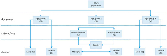
Figure 1.
Weighted proportion structure of the city’s main parameters: age group, labour force composition and gender structure.
- Capacity, fairness of allocation and rounding number
We apply the capacity model based on the Amsterdam’s age groups share in Figure 1 for selecting which household profiles to be modelled. The main goal is to determine the number of the occupants’s profiles to be modelled as shown in the following expression of Equation (5):
where Tamt is the total number of the occupants’ profiles. AG1wt is the number in age group 1 based on it’s weight. AG2wt is the number in age group 2 based on it’s weight and AG3wt is the number in age group 3 based on it’s weight. The share of the occupants for each group are converted to decimal form to provide the results of the total number of occupant-profiles from each age group.
Furthermore, the capacity model can also be extended to determine the gender of the selected profiles as expressed in Equation (6) if it is supported by the profile generators. In this case, it is applicable to LPG, since LPG provides detail characters of the occupants’ gender information:
Here Tg is the total number of combinations of the occupants’ gender. AG1m is the share of males in age group 1. AG1f is the share of females in age group 1. AG2m is the share of males in age group 2. AG2f is the share of females in age group 2. AG3m is the share of males in age group 3 and AG3f is the share of females in age group 3. In this case a widely used fairness sharing technique called max-min fairness can be applied in sharing the allocations if it is required.
Therefore, the application of the Wepro model to the case-study city namely Amsterdam is as follows: First, the city’s population is represented by the sum of the composition of age groups in Amsterdam. We grouped the city’s age groups into three categories: 0–17 years old = 17.5%; 18–64 years old = 70.3%; and above 64 years old = 12.2% [57,58] using the formula in Equation (1):
In more detail, the gender structure is classified into three age groups. For the age group of 0 to 17-year-olds, 51.58% are male and 48.42% female. In the age group of 18- to 64-year-olds, 50.24% are male and 49.75% female. Finally, for the age group above 65, we identified 46.24% male and 53.75% female [57,58]. Therefore, Equation (2) is presented to identify the gender at the city level:
Furthermore, the labour force data are measured on the basis of the labour force population, which is only derived from age group among 18- to 64-year-olds. The unemployment rate is recorded as 6.7% [56]. In this case, Equation (3) is used to identify the employment and unemployment shares.
Here, Equation (4) is used where the labour force is the proper set of age groups, labour force being an aspect of the age groups but not equal to age groups:
AG = { 0–17 years old, 18–64 years old, 64+ } and LF = { 15–64 years old }
We coupled the share of age groups and labour force and applied the Proportional matched profile to the total population as the city’s main characteristics. Therefore, as displayed in Figure 2, the Amsterdam’s main profile should reflect: The age groups, labour force and gender classes.
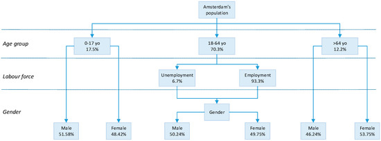
Figure 2.
The application of the Weighted proportion (Wepro) model’s structure to the case-study city, namely Amsterdam, The Netherlands. It consists of the Amsterdam’s age group share, labour force composition share and gender share of each age group.
This means that from the age group percentage: The aged 0–17 group is nearly 20%, aged 18–64 is 70% and the rest 10% is for aged over 64. From this 70% where the aged 18–64, there is about 93% of this age group are people with work and the rest are not working. Furthermore, each age group illustrates a slight difference in the share of gender information, except for the aged over 64, where the female populations are slightly more dominant than the male populations.
- Capacity, fairness of allocation and rounding number
Furthermore, Equation (5) is presented, where the weighted city’s age group values are applied into a simple capacity model, in order to determine the capacity of the allocation. Therefore, based on the weighted values, we have ten capacity of the households profiles. It means, we can only select maximum ten occupants from the household profiles generators:
Furthermore, if it is supported by the profile generators, the capacity model can also be extended to determine the gender of the selected profiles as expressed in Equation (6). In this case, it is applicable to LPG, since LPG provides detail characters of the occupants gender information:
As shown in the Equation (5), age group 1 has two allocations, age group 2 has seven allocations and age group 3 has one allocation. Thus, there are currently two resources for two allocations, which after the division between them, resulting in 1. Furthermore, has an excess of 0.03, where the excess can be taken and divided among the remaining demands, which is only AG1f. Therefore, AG1f = 1. As a result of the capacity and fairness of allocation model depicted in Figure 3, there will be two occupants: one male and one female in age group 0–17. Furthermore for the case Age group 2 and Age group 3, we cannot fully apply the max-min fairness. We simply apply rounding number because we have only two resources per age group. For instance, for age group 3, there are two resources for only one allocation. Therefore, rounding number is applied to the highest weight between the resources.
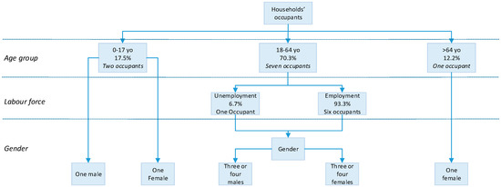
Figure 3.
The application of the Wepro model’s structure to the case-study city, namely Amsterdam, The Netherlands. It consists of the Amsterdam age group share, labour force composition share and gender share of each age group and their capacity of the occupants to be modelled.
As a result, the age group 18–64 should consist of seven adult occupants with six of them working people and one person not working. Considering the gender share is quite balance in this age group, then it is either four females and three males, or four males and three females in the occupants’ list. Lastly, for the aged over 64, which has only one allocation, based on the results of the capacity and fairness of allocation model, we apply rounding value to the one which has the highest share to represent the senior age group. Therefore, we selected a female senior to represent this age group.
2.1.2. Profile Generators: LPG and ALPG
To produce the load profiles of the selected households profiles as the result of the Wepro model between the city’s main characteristics and the households occupants, we use LPG and ALPG as the load profiles generators. Thus, in this case we optimise a bottom-up approach provided by the generators, scale-up from the household level to the city level based on the down-scale task perform previously in the weighting model, and employ the profile generator’s model at the former level.
The main reason of choosing LPG and ALPG because both of them are developed based on behavioral model, which is in line with ClairCity project’s goal to model the citizen’s behaviour. LPG’s model has been selected for use in our model, as it offers a mature model with which to synthesise household energy load profiles based on various occupants’ profiles. Pflugrandt has developed the model with a strong focus on modelling the behavioural aspect. The basic elements for modelling a single household in Figure 4 are the desire to do so and expressions of the need to do something. The model specifies weight, threshold and decay time as desired properties [15].
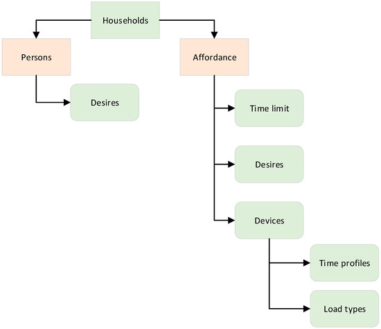
Figure 4.
LPG’s minimum necessary elements in modelling a decision-making process of a single household [15], where the basic elements are the desire to do so and expressions of the need to do something.
Weight is the relative weight of a need compared to all a person’s other needs. In selecting for the next action, the minimisation of the deviation requirement is used as a criterion, the weighting acting as a multiplier in this calculation. Threshold determines when the person really feels a need, that is, when it is included in the next action selection of the calculation. For example, in reality there is usually no eating after lunch because only 10% of the hunger sensation is evident. Instead, one generally waits until a noticeable feeling of hunger has built up before having dinner. Finally, Decay Time describes the half-life, until 50% of the requirement is reached. It has been found that activities at 50% threshold mostly after the two to three times the decay time, depending on the weighting and the other available activities. The decay constant is calculated from the decay time by which the current value of the need is multiplied in each time step [15]. When creating households, it has been found that activities at the 50% threshold are usually executed after two to three times the decay time, depending on the weighting and the other available activities. Furthermore, besides desire, it is also essential to identify the individual’s properties (age, gender, sick leave in the year, average duration of illness, needs when healthy, needs when ill) and load type, which in this case is electricity [14,15]. LPG provides various pre-defined German household profiles.
The second profile generator used in our work is ALPG. ALPG employs household occupancy profiles generated by a simple behavioural model, which creates consistent profiles for the devices. The devices’ flexibility is specified through four classes: timeshiftables, buffer-timeshiftables, buffers and curtailable. The inflexible electricity profiles are grouped into the following categories: stand-by load, consumer electronics, lighting, inductive devices, fridges, and other. Furthermore, to show annual electricity consumption, the individual profiles are scaled in magnitude, making it easier to alter the profile if there is a change in electricity usage by the external factors. An example of such a change could be the adoption of a new technology, for instance, light-emitting diode (LED) lights. Moreover, the following classes in Figure 5 are implemented in the simulation model: neighbourhood, household, person, device, house, writer and ALPG. Electricity usage in a typical Dutch setting is the focus of ALPG, which is also in line with our work in modelling residential electricity load profiles, with Amsterdam as the case-study city [16,17].
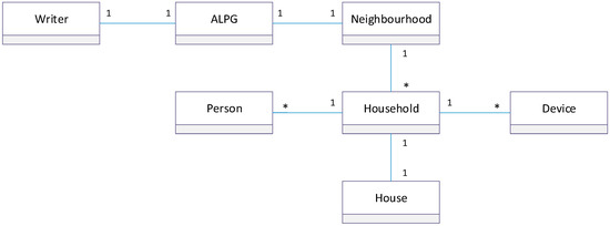
Figure 5.
ALPG’s class diagram [17] that shows the cardinality of a class in relation to another. The example of one-to-one (1..1) relationship is depicted between Household and House, where a household lives in a house and a house belongs to a household. The one-to-many(1..*) relationship is shown between Household and Device, where a household has one or more devices, and each device belongs to a household. Each class from these multiple classes represents a part of the model, which makes the software flexible to be extended in the future work.
Furthermore, we after applying the capacity allocation into LPG and ALPG the following are closest profiles that reflect the city’s proportion of the age groups, gender and labour force mentioned above.
- LPG
The following are the simplified Wepro-based selected pre-defined households profiles in LPG although there could be also several other options that may fulfill the Wepro model composition:
- Couple, both of whom work, with one child
- Couple,one at work, one at home, with one child
- Coupleboth of whom work
- Singlewith work
- Seniorat home
The underlined entities indicate the age groups, the blue italic entities represent the labour force. Moreover, to express the gender shares of each age group, we selected the characters of LPG pre-defined household profiles in Table 3, as follows:
Table 3.
The selected pre-defined household profiles in LPG based on Wepro model.
Furthermore, we can insert these occupant’s list to the Wepro composition in order to validate the model. As illustrated in Figure 6, the selected household profiles can fulfill the Wepro’s model composition. Then, we generate these LPG’s pre-defined households’ load profiles one by one. The LPG can be downloaded free from https://www.loadprofilegenerator.de/. In generating one pre-defined household’s load profile, after we download and open the windows program, we can go to “calculation” menu.
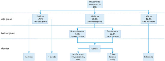
Figure 6.
The application of the Wepro model’s structure for Amsterdam’s household occupancy profiles in LPG. It consists of the Amsterdam’s age group share, labour force composition share and gender share of each age group, their capacity of the occupants to be modelled and the selected gender character provided in LPG.
Furthermore, we should select some options such as which pre-defined profile to be modelled, geographic location and temperature profile based on temperature dataset that we input before, if the temperature dataset is not provided yet by LPG. That is why we need to pre-process our input data such as temperature dataset in order to be matched with LPG’s format. Then we can calculate the household profile one by one which may require a computational processing time and the result is generated in comma-separated values (.CSV) file.
- ALPG
As shown in Table 4, the pre-defined households profiles in ALPG are not as detailed as in LPG, but they simply can fulfill the Wepro model. The pre-defined households class contains seven types of households: Single worker, dual worker, family dual worker, family single parent, dual retired and single retired. Dual profile means a couple. In this case, each type of household corresponds to a category of electricity annual consumption in Kilowatt hour and amount of occupants or persons.
Table 4.
Pre-defined households configurations in ALPG based [17].
To fulfill the Wepro model and simplify the process, we selected: one single worker, one single retired, two dual worker and one family dual worker. ALPG is open-source code and the code is available at it’s github page. Figure 7 shows the snipped code of the households profiles selection, where the ALPG program runs by executing profilegenerator.py.:
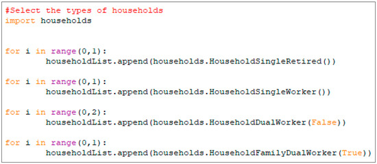
Figure 7.
The snipped code of the configuration of the selected household profiles in ALPG based on Wepro model.
Furthermore, the same procedure with LPG, in Figure 8 we inserted these occupant’s list to the Wepro composition in order to validate the model.
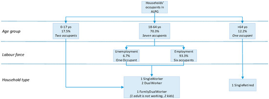
Figure 8.
The application of the Wepro model’s structure for Amsterdam’s household occupancy profiles in ALPG. It consists of the Amsterdam’s age group share, labour force composition share and gender share of each age group, their capacity of the occupants to be modelled and the selected pre-defined profiles provided in LPG.
Accordingly, it indicates a different result in comparison with LPG because in ALPG there is no need to identify the gender characteristics as it has simplified and consistent pre-defined profiles list as provided in Table 4. Moreover, these selected occupancy’s list in ALPG may fulfill the Wepro model regardless the gender detail. In consequences, there are five generated households load profiles both in LPG and ALPG. We used the average load profile’s value of these generated load profiles in the analysis.
2.2. Load Profile Analyses Based on Time-Division
As the model has produced residential electricity load profiles in high resolution, we focus on analysis of the load profile results in this section. The visualisation, charting and plotting of the hourly resolution are executed in Python. The residential electricity load profile is analysed at four levels: seasonal analysis, monthly analysis, days analysis and hourly analysis.
2.2.1. Seasonal Analysis
Electricity consumption patterns based on the seasons is interesting to distinguish, as the temperature influences the interval of the seasons. A time-division according to the four seasons in the year has been defined based on the meteorological concept (Table 5).
Table 5.
Division of the seasons based on meteorological concept in the selected year: 2015 (date format: dd-mm-yyyy). In this case, the start day of the winter season is 01 December 2015. Winter lasts from 01 December 2015 until 28 February 2015, spring lasts from 01 March 2015 to 31 May 2015, summer lasts from 01 June 2015 to 31 August 2015, and autumn from 01 September 2015 to 30 November 2015. Therefore, the winter season has the fewest number of days.
The meteorological concept (Table 5) is quite simple and is the most widely used, being broken down into four three-month periods. Winter has the three coldest months in the Northern Hemisphere, namely December, January and February. Spring runs from March to May, summer from June to August, and the other months belong to autumn [59]. Hence, a seasonal electricity load profiles model is proposed as follows in Equation (7):
where Ts% is the total of seasons share, Sw% is the share of Winter season, Ssp% is the share of Spring season, Ssm% is the share of Summer season and Sa is the share of Autumn season.
2.2.2. Monthly Analysis
Monthly characteristics are examined through the monthly average share to identify the monthly pattern of residential electricity consumption in the city. The analyses cover the 12 months electricity data from the load profiles results. Besides to identify the potential energy savings, the monthly analysis is beneficial to plan the generation and distribution of power utilities.
2.2.3. Days Analysis
The days analysis is provided based on the hourly average share load of the days in each season and the typical days share in each season. The typical days are the selected days, of one weekday and one weekend day in each season as listed in Table 6. None of the selected days listed below in Table 6 is a national holiday in the selected city, meaning that the selected days represent people’s normal daily activities on a weekday and at weekends.
Table 6.
Selected typical days (date format: yyyy-mm-dd).
2.2.4. Hourly Analysis
In this part, we will process the output from the load profile generators as one minute resolution and create a time series with an hourly resolution. The objective is to show the hourly characteristics of electricity consumption on the hourly average load profiles in the selected year and the hourly average of the seasonal load profiles. Hence, the average load profiles model is proposed as follows in Equation (8):
where is the hourly average. n is the number of hours which is in the range of 0 to 23. is the number of days in a year, which is in the range of 1 to 365 for the selected year 2015. is the data i-th. To create the hourly average of the seasonal load profiles, we replace with the number of the days in each season.
3. Results: Load Profile Analyses in Amsterdam as the Case Study
The analyses of the generated load profiles by the model will be presented based on the time variation of the case-study city, namely Amsterdam (The Netherlands). The hourly temporal results will be moderately validated by the standard average of Dutch household load profile.
3.1. Load-Profile Analyses Based on Time-Division
The generated load profiles produced by the model will be analysed at four levels: seasonal analysis, monthly analysis, days analysis and hourly analysis, where hourly resolution is the core output of our temporal profile.
3.1.1. Seasonal Analysis
The seasonal variations based on the meteorological concept (Table 5) are provided in two generated models: Wepro-LPG and Wepro-ALPG, where we used Equation (7). In this concept, Winter has the fewest days, Autumn has one day more compared to winter, while spring and summer have two days more compared to winter. Based on the generated load profiles of Wepro-LPG and Wepro-ALPG in Figure 9, it indicates that Winter is the highest consumption share, slightly followed by Autumn, and Spring. Both models show Summer as the lowest consumption share.
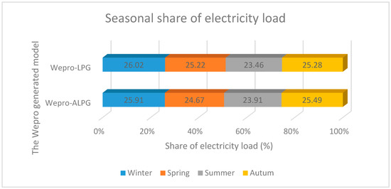
Figure 9.
Seasonal share of electricity load based on the models: Wepro model-LPG and Wepro-ALPG. Both models show similar seasonal characteristics of the consumption share from the highest season to the lowest season.
Wepro-LPG
while for Wepro-ALPG, the highest consumption share occurred in winter, slightly followed by autumn, then spring. Summer is recorded as the lowest consumption period.
Wepro-ALPG
3.1.2. Monthly Analysis
Amsterdam’s monthly electricity load share is illustrated in Figure 10, which shows a distinct profile in the Wepro-LPG model. This demonstrates that December has the highest consumption share compared to the other months, which may exhibit seasonal variations. Surprisingly, this load profile identifies May as having the second highest electricity share in 2015, followed by October, August and January. The lowest monthly consumption share is in July, which concurs with the seasonal analysis result that summer has the lowest consumption share in all load profiles. The second lowest consumption share is in March, followed by September.
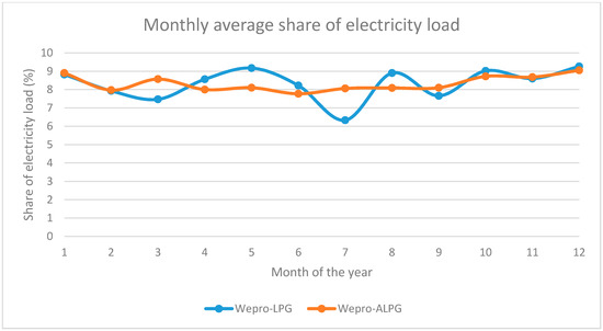
Figure 10.
Monthly average electricity load share based on the results of the generated Wepro-LPG and Wepro-ALPG models.
The Wepro-ALPG model indicates December as having the highest consumption share, the same as in Wepro-LPG model. The second highest consumption share is in January, followed by October and November. The lowest consumption share is in June, followed by February and April.
3.1.3. Days Analysis
The days analysis is provided based on the hourly average share load of the days in each season which are depicted in Figure 11, and the daily load share of the typical selected days, which is illustrated in Figure 12.
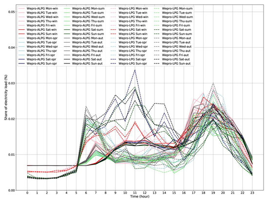
Figure 11.
The hourly average load share of the days in each season of Wepro-LPG and Wepro-ALPG models.
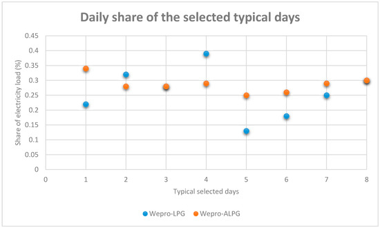
Figure 12.
Daily share of electricity load of the selected typical days in each season based on the results of Wepro-LPG and Wepro-ALPG load profiles.
Figure 11 depicts the hourly average load share in each season based on the days Monday, Tuesday, Wednesday, Thursday, Friday, Saturday and Sunday, where the load profiles for Wepro-LPG are shown in dashed lines and the load profiles for Wepro-ALPG are shown in solid lines. The Winter load profiles are shown in red, the Spring load profiles are shown in blue, the Summer load profiles are shown in green and the Autumn load profiles are shown in black, where the weekday colours are in a lighter shade then the weekend colour.
For the winter period in Wepro-LPG, the top morning peak appears around 7 am for all weekdays. For some weekdays, the morning peak then continues with a light peak between 9 am and 10 am. The following daylight peaks are identified around lunchtime, from 12 am to 1 pm, while for weekend days, the curve show several daylight peaks from 7 am to late lunchtime, around 1 pm. The morning and daylight peaks appear around 7 am, 9 am, 11 am and 1 pm, among which 11 am is identified as the top morning peak, which may be associated with the brunch time. Furthermore, the evening peaks for all days started from about 5 pm to 8 pm and mostly reach the top value around 7 pm, while for the weekend days, the curves show a longer evening peak from 6 pm to around 7:30 pm. The weekend days show a quite higher daylight share than the weekdays’ daylight share. Furthermore, for Wepro-ALPG, the top morning peak is shown around 7 am for all weekdays, followed by a light peak around 8 am on some weekdays. For some weekdays, the morning peak then continues with a light peak between 10 am to 12 am. The load share continues to increase until 2 pm, while for the weekend days, the morning peaks are characterized by a light peak around 7 am that continues to increase to 10 am. The top morning peak is around 12 am. The weekend days show a higher daylight share than the weekdays’ daylight share. Most of the days indicate 6 pm as the top evening peak, some weekdays identify 5 pm as the top evening peak and one weekend day shows 7 pm as the top evening peak.
The hourly average load share in Spring period for Wepro-LPG illustrates the top morning peak around 6 am for all weekdays. The following morning and daylight peaks occur around lunchtime from 12 am to 2 pm, while for weekend days, the curves show several morning peaks from 6 am to late lunchtime around 2 pm. The morning and daylight peaks are shown around 6 am, 9 am, 11 am and 2 pm, where 11 am is identified as the top morning peak, which may be associated with brunch. Furthermore, the evening peaks for all days start from about 6 pm to 8 pm and mostly reach the top peak around 7 pm. It is obvious that the weekend days show a quite significant higher daylight share than the weekdays’ daylight share. Furthermore, the hourly average load share in Spring period for Wepro-ALPG shows the top morning peak around 7 am for all weekdays, followed by a light peak around 8 am on some weekdays. For some weekdays, the morning and daylight peaks then continue with a light peak at 10 am, 11 am, 1 pm and 2 pm. After 7 am, the curves are continually declining until 9 am. The load share continues to increase again with a slight share from 9 am to 2 pm, while for the weekend days, the morning peaks start with a slight peak from 7 am, and gradually increase to reach the top on 10 am. It then increases slightly at 12 am, which is identified as the top morning peak in the weekend days. The weekend days show a higher daylight share than the weekdays’ daylight share. Most of the days indicate 6 pm as the top evening peak, one weekday identifies 5 pm as the top evening peak and some days shows 7 pm as the top evening peak.
Furthermore, the Wepro-LPG in Summer period indicates the top morning peak on 6 am and 7 am for all weekdays. The following morning peak is around 10 am to 2 pm, while for weekend days, the curve shows several morning and daylight peaks from 6 am to late lunchtime, around 2 pm. These peaks are evident at 6 am, 7 am, 8 am, 11 am and 2 pm, where 11 am is identified as the top morning peak, which may be associated with brunch. Furthermore, the evening peaks for all days have started from about 6 pm to 8 pm, which all days reach the top peak on 7 pm. The weekend days show a quite significant higher daylight share than the weekdays’ daylight share, while for Wepro-ALPG in Summer period, the top morning peak is shown around 7 am for all weekdays, followed by a light peak around 11 am for most weekdays. The load share continues to increase again with a slight share from 11 am to 2 pm, while for the weekend days, the morning peaks start with a slight peak at 7 am, then a gradual slight one increasing each next hour and reaching the top on 10 am. It then slightly increases further at 12 am. The weekend days show a higher daylight share than the weekdays’ daylight share. Most of the days indicate 6 pm as the top evening peak, two weekdays show 5 pm as the top evening peak and the weekend days shows 7 pm as the top evening peak.
Furthermore, the hourly average load share in Autumn period for Wepro-LPG illustrates the top morning peak on 6 am on most weekdays and one weekday has 7 am as the top morning peak. The following morning peak occurs on 10 am on most weekdays, followed by another daylight peak at 2 pm, while for the weekend days, the curve identifies several peaks at 6 am, 8 am, 9 am and 11 am. The morning peaks are seen around 6 am, 9 am, 11 am and an afternoon one at 2 pm, where 11 am is identified as the top morning peak, which may be associated with brunch. Furthermore, the evening peaks for all days start to increase from about 5 pm or 6 pm and all days reach the maximum evening peak on 7 pm. It is obvious that the weekend days show a quite significantly higher daylight share than the weekdays’ daylight share. Lastly, the hourly average load share in Autumn period for Wepro-ALPG shows the top morning peak around 7 am for all weekdays, with a slight peak occurring before at 6 am. The next peak happens at 10 am, with the load share increasing gradually from 11 am to 3 pm on all weekdays, while for the weekend days, the morning peaks start with a slight peak at 7 am, and the load share keeps increasing until it reaches another peak at 10 am. It then increases further to reach the top morning peak at 12 am. The weekend days show a higher daylight share than the weekdays’ daylight share. Most of the days indicate 7 pm as the top evening peak, one day identifies 5 pm as the top evening peak, another day shows 6 pm as the top evening peak and another day has 8 pm as the top evening peak.
In addition, as an overview of the daily total share load, we present the selected typical days analysis in Figure 12, where the selected days represent weekdays and weekend days of each season.
For the weekdays, we selected 1: 11 February 2015, 3: 15 April 2015, 5: 15 July 2015 and 7: 11 November 2015. The load profile of the Wepro-LPG model in Figure 12 shows that 15 April 2015 has the highest consumption share among the selected weekdays, followed by 11 November 2015, 11 February 2015 and 15 July 2015. For the weekend days, we chose 2: 15 February 2015, 4: 19 April 2015, 6: 19 July 2015 and 8: 15 November 2015, showing that 19 April 2015 has the highest consumption share among the selected weekend days, followed by 15 February 2015, 15 November 2015 and 19 July 2015. Weekdays and weekends both show that the lowest consumption share is in the selected days in July, which concurs with the seasonal and monthly analyses. In addition, this also shows that the weekends have higher consumption shares than the weekdays.
In the Wepro-ALPG model, the load profile indicates 11 February 2015 as having the highest consumption share among the selected weekdays, followed by 11 November 2015. 15 April 2015 comes next, but with only a subtle difference. The lowest share is on 15 July 2015. The Wepro-ALPG model for weekends shows 15 November 2015 as having the highest consumption share, followed by 19 April 2015, then 15 February 2015, then 19 July 2015. Both Wepro-LPG and Wepro-ALPG are having the same values on 15 April 2015 and 15 November 2015.
3.1.4. Hourly Analysis
The hourly average load profiles in a year are provided in Figure 13 based on the expression in Equation (8). Figure 13 also illustrates the seasonal hourly average load profiles, where the load profiles for Wepro-LPG are shown in dashed lines and the load profiles for Wepro-ALPG are shown in solid lines. The Winter load profiles are shown in red, the Spring load profiles are shown in purple, the Summer load profiles are shown in green and the Autumn load profiles are shown in blue, where the hourly average load profiles in a year are shown in grey bold lines.
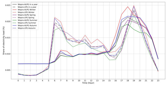
Figure 13.
The hourly average load share in a year and the hourly average load share in each season based on the results of Wepro-LPG and Wepro-ALPG models.
The Wepro-ALPG curve illustrates an increasing load from 5 am and reaches the morning peak around 7 am. Then, the load decreases gradually until 9 am and increases again to 10 am. After that, the curve remains flat from 10 am to 1 pm although there is a subtle peak in between around 12 am or during lunchtime. It is then increases slightly from 1 pm to 3 pm, and after 3 pm the curve is increasing significantly and is reaching the evening peak around 6 pm. Furthermore, after 6 pm the curve is decreasing gradually until midnight. After that, the curve remains flat until 5 am. While for the Wepro-LPG, the morning peak starts to increase significantly from 5 am and reaches the peak at 6 am. After 6 am, the curve is gradually decreasing until 4 pm although there is a subtle peak around 11 am. It starts to increase again significantly and reaches the evening peak at 7 pm. The curve decreases significantly after 7 pm to midnight. Furthermore, it remains quite flat until 3 am. There is a slightly increase load between 3 am to 5 am before the morning peak.
Furthermore, the hourly average load per season for both models indicate the consistent curve shape within the season and model, either Wepro LPG or Wepro ALPG. The winter curve indicates the highest load profile among the hourly season curves, and it is more obvious for Wepro-ALPG whereas the winter’s curve is shown as the highest load and slightly followed by autumn’s curve for Wepro-LPG. The demand peaks show similarity with the hourly average in a year as the top peak is in the evening, followed by the morning peak and a subtle peak during the lunch time, with both models identifying the same peak hours as the peak hours for the hourly average in a year. In general, Wepro-LPG’s load profiles for all seasons have higher load share than the Wepro-ALPG’s load share for all seasons during the day. Conversely, the Wepro-ALPG’s load indicate longer peak share than the Wepro-LPG’s load during the night time.
3.2. Validation with Case Study’s Measured Data
Validation can be done by comparing the data generated by Wepro with the city’s measured data such as smart-meter data, TUS data or data from the utilities. In this case, we cannot make an in-depth validation as the measured city’s data is unavailable. Therefore, a future study would follow to improve our current work when the city’s measured data is available.
In practice, we can still compare our model with the standard load profiles for Dutch households published by the Energy Data Services Netherlands (EDSN) to validate whether our hourly average generated load profiles have the same trends the standard Dutch residential load profile. The average normalised standard household load in The Netherlands based on EDSN is provided in Figure 1 of [11]. It is shown that the morning peak starts to increase from 5 am, similar to both our generated models. It then reaches the peak around 10 am, while both our models identify the morning peak around 6 am to 7 am. The EDSN’s load remains flat from 10 am to 13 pm, although there is a subtle peak at 12 am during lunchtime. This curve from 10 am to 13 pm is quite similar to the Wepro-ALPG model one. Furthermore, like the Wepro-LPG model, the ESDN’s load is decreasing gradually to 4 pm. After that, the curve starts to increase significantly like the curves of both our generated models. The EDSN’s model reaches the peak between 19:00 and 19:30 similar to the Wepro-LPG. Furthermore, the load is decreasing quite significantly until 2 am. It remains flat from 2 am to 5 am which is similar to our generated models. In general, it can be concluded that the generated hourly average share of the Wepro models have similar curve trends as the EDSN’s load trend, although the morning peaks in the generated Wepro models have different time characteristics from EDSN’s morning peak. Furthermore, both our models and the EDSN’s model show a subtle peak during lunchtime. The evening peak occurs after dinner in the Wepro-LPG and EDSN model, while the the evening peak is occurring exactly at the dinner time in Wepro-ALPG.
As an update, the load profile data in EDSN have been moved to de Vereniging Nederlandse Energie Data Uitwisseling’s (NEDU) page [33]. The data provided in NEDU’s page start from year 2016, therefore data 2016 are used in this initial validation. Smart-meter data is used as a basis for the consumption/production profiles as described in ‘Profielenmethodiek elektriciteit’, where the documentation is available in Dutch. The raw data are provided in 15 min resolution, which show how much electricity is allocated in that 15 min. The data are obtained from 3,002,450 households type E1A in 2016. The comparison of the standard average Dutch household load profile in 2016, which has similar trends with Figure 1 of [11] for E1A residential type and the hourly average load profile in a year of Wepro-LPG and Wepro-ALPG is plotted in Figure 14.
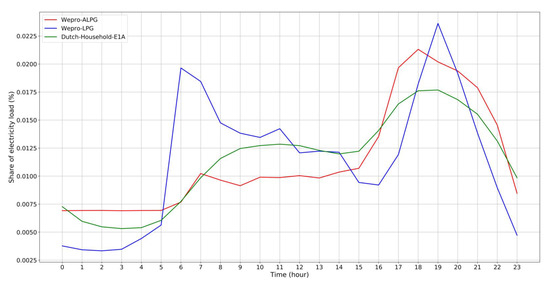
Figure 14.
The comparison of hourly average standard residential load profile in The Netherlands based on NEDU’s data of 2016, E1A and the hourly average load profile in a year of Wepro-LPG and Wepro-ALPG.
This simple validation is an initial check to see whether our generated load profiles resemble the standard Dutch’s household load profile characteristics before going into an in-depth validation with the city’s measure data. Moreover, further study in the future is required.
4. Discussion
Based on the results, our weighted proportion (Wepro) model can be applied to generate the residential electricity load profiles at the city level by utilising the exisiting household profile generators, either LPG or ALPG, which we have employed here, given that they both have specific behavioural profile models. The seasonal share analysis based on Wepro-LPG and Wepro-ALPG, shows each season’s consumption share is in the range of 23% to 26%. The 1% share consists of approximately 80 h of load or about 3 days of load when calculated on the basis of the hourly dataset. For instance, if we compare the winter and summer seasons to the whole year in Wepro-LPG as shown in Figure 9, where winter is 26.02% and summer is 23.46%, it indicates that the electricity load in winter is almost 3% higher than in summer to the whole year, which is equal to approximately 240 h or about 9 days. In addition, both seasonal profiles indicate Winter as having the highest consumption share, which concurs with the known seasonal pattern in energy demands studies [60,61,62]. In addition, the seasonal analyses based on meteorological is important to be mentioned as some studies did not mention which time-division concept they used for analysing the seasonal electricity profile. Furthermore, the monthly analysis results illustrate that December is having the highest consumption share, which accords with the result of some monthly electricity studies [61,63].
The hourly average share based on the days in each season show that the weekend days indicate a higher daylight share than the weekdays’ daylight share in both models. The result of the daily share of the selected typical days for all models indicates that most weekend days have a higher consumption share than weekdays in the same season. It concurs with an analysis of weekday and weekend variation, where weekend days show slightly more electricity use than weekdays [64]. Exception found in the Wepro-ALPG model’s selected days in winter, where weekday consumption is higher than at weekend.
The hourly average load profiles identify the morning and evening peaks in Wepro-ALPG and Wepro-LPG, where the Wepro-LPG model has a higher load than the Wepro-ALPG model for both peaks. It is also identified that the evening peak has a significant higher load value than the morning peak load value in both models. All the hourly average loads in a year and per season demonstrate a consistent curve shape within season and model, either Wepro LPG or Wepro ALPG. The consistency is also shown within the curve shape of the hourly seasonal average load share with the hourly seasonal load share based on the days within the model.
As a consequence, the application of our model requires a profile generator as an external tool to match the weighted city’s profile with the representative occupants’ profiles at the household level, since we are not building our own profile generator. It also influences the results of the generated load profiles where they will be based on the characteristics of the developed model in profile generator, include relying on the few selected input profiles as a result of the approach taken in this study. The issue of relying on the few selected input profiles may result in the less fluctuations load profiles as shown in the Wepro-ALPG load profiles for the morning curves. The main difference of the hourly average in a year between the models is shown in the morning curve, where for Wepro-LPG after reaches the peak on 6am, the load share is declined gradually until 4 pm, with some light peaks in between, while for Wepro-ALPG, the curve declines slightly until 9 am after reaching a peak at 7 am. It increases again at 10 am and remains stable until 1 pm. This issue is also has been initially identified in [16] where the generated profiles show less fluctuations on the single household level, while the fluctuations at the neighbourhood level matched with the measured values. We assume that the less fluctuations during the morning period generated in Wepro-ALPG might be caused by the consistent pre-defined profiles in ALPG, where they are developed based on the simple behavioural model of an occupancy profile. The occupancy model for general events in ALPG is configured using mean times to change the state of a person. In this case, it is limited to the three person’s states: active (being home), inactive (e.g., sleeping) and away (e.g., to work) [16], while in the generated load profiles of Wepro-LPG, the fluctuations are obviously shown during the morning period which might be caused by the detailed behavioural model that emphasised on the person’s desire developed in LPG model. Although, it requires a future analysis. In general, the Wepro-ALPG has more aligned curve shape with the average standard Dutch residential load profile as illustrated in Figure 14 than the Wepro-LPG, where it could be because ALPG model is built based on Dutch dwelling setting. Moreover, a measured dataset that adequately represents the case study is required for validation purposes although in general our generated hourly average load profiles have similar curve’s trend with the standard Dutch residential load profile provided by NEDU.
In addition, our model is found to be more efficient in respect of its computational time. In this case processing the load profiles of the city’s residential sector, which consists of a large number of households is more efficient rather than generating each household in LPG or a certain number of city’s households in ALPG. It takes about ten minutes computation to generate a single-person household load profile in LPG and about fifteen minutes computation to generate a multi-occupants household load profile in LPG, for instance profile: Family, 3 children, both adults at work. Thus, in takes 60-min to generate the Wepro’s selected five profiles of Table 3 in LPG, where we used LPG version 8.9.0. Furthermore, the simulation of the current configuration that consists of five households from four types of pre-defined profiles in ALPG takes about eight minutes. We use Python 3.7 (64-bit) to run this configuration. All of these simulations either LPG or ALPG were conducted on a computer using an Intel core i5-5300U CPU processor @2.3 GHz and 8 GB of installed memory (RAM). Thus, the computation will take much longer than our approach to generate a single or the few load profiles at the city level. In this case, our approach to model the residential sector at the city level has also tackle the limitation addressed by the ALPG that the tool is aimed at small group of houses which is maximum about 100 households per simulation. Consequently, our approach also creates efficiencies in the size and storage of the generated files. For instance, the output folder of one “single with work” profile generated in LPG has 2.6 GB size and the output folder of our selected pre-defined profiles in ALPG has 1.5 GB size.
5. Conclusions
This work has developed a simplified and practical approach to model residential electricity load profiles where the model can match the main city’s characteristics with the representative pre-defined households profiles proportionally. The Wepro model is advantageous as an efficient approach to develop the residential electricity load profiles at the city level, especially where survey data, smart-meter data or any other local temporal profiles dataset are unavailable. The findings concur with some load profile studies from the similar climate profile which indicate Winter as the highest consumption share and illustrate either December or January is having the highest consumption share. The results of the selected typical days for all load profiles indicate that most weekend days have a higher consumption share than weekdays in the same season. Moreover, all the hourly average load profiles in a year and per season demonstrate the consistent curve shapes, demand peaks and the peak hours within the season and model, either using Wepro-LPG or Wepro-ALPG. In terms of the curve shape and daylight characteristics between the models, the hourly average in a year of Wepro-ALPG is preferred to be used because it also shows a high similarity with the shape of the standard Dutch household provided by NEDU or previously EDSN, although the Wepro-ALPG load profiles illustrate less morning fluctuations as a result of the few input profiles taken by the approach. In addition, in terms of the evening peak, the hourly average in a year of Wepro-LPG is preferable to be used, because it resembles the evening peak time of the Dutch household characteristics, where the evening peak takes place after dinner time, which concurs with a Dutch load profile study that the evening peak takes place after dinnertime when e.g., TV, dishwasher, etc., are on because within the average Dutch household, cooking is done using gas instead of electricity.
Moreover, our work contributes by evaluating the characteristics of residential electricity load profiles based on time variation analyses: seasonal analysis, monthly analysis, days analysis and hourly analysis. In addition, this method is applicable to model previous year, current year and future year, where for current year and future year are used city’s projected numbers.
Furthermore, the few selected household profiles which are the representative of the city’s profile may dominate the shape of the output profiles where all of input have represented the city’s age group, labour force composition and gender share. Although the few selected profiles may dominantly influence the output profile, based on the results, they still resemble the Dutch average household profile and concur with the common peak demands characteristics. In addition, although the Wepro model depends on external household profile generators such as LPG and ALPG, the Wepro model is found to be more efficient in storage capacity and computational process of the residential sector’s load profiles, given the number of households in the city that can represent the local profile.
In future work, it would be interesting to identify the potential of energy savings based on the generated load profiles using a relevant machine-learning technique. We also look forward to add more main input parameter to the model and compare with the case study’s measured data. Further work might also be conducted to extend residential electricity temporal profiles into spatial profiles.
Author Contributions
The idea, method and analysis of the study is designed by A.K. A.K., P.D.K.M. and P.S.N. wrote the paper. P.D.K.M. performed the complex pre-processing and modelling tasks in Python. P.S.N. reviewed and proofread the paper. All authors have read and agreed to the published version of the manuscript.
Funding
The research described in this paper is being conducted as part of the ClairCity project, funded by the European Union’s Horizon 2020 research and innovation programme under grant agreement No. 689289, and a PhD fellowship within the CITIES project at Denmark Technical University (DTU) funded by the Indonesia Endowment Fund for Education (LPDP) under Letter of Guarantee: Ref:S-1401/LPDP.3/2016. The CITIES project is funded by InnovationsFund Denmark under contract: 1305-00027B.
Acknowledgments
We acknowledge ClairCity partners within the Technical work package UWE–United Kingdom, TML-Belgium, UAVR-Portugal, Techne-Italy, NILU-Norway, PBL-The Netherlands, CBS-The Netherlands, and other partners for supplying the related datasets and other large-scale inputs. We also acknowledge Noah Pflugradt for developing and publishing the LPG, and Gerwin Hoogsteen, the University of Twente, The Netherlands for developing and publishing ALPG. Furthermore, we thank Elke Klaassen for sharing her publication and The Netherlands’ load profile information.
Conflicts of Interest
The authors declare no conflict of interest.
References
- Daioglou, V.; van Ruijven, B.J.; van Vuuren, D.P. Model projections for household energy use in developing countries. Energy 2012, 37, 601–615. [Google Scholar] [CrossRef]
- Pablo-Romero, M.d.P.; Pozo-Barajas, R.; Yñiguez, R. Global changes in residential energy consumption. Energy Policy 2017, 101, 342–352. [Google Scholar] [CrossRef]
- Zuo, C.; Birkin, M.; Malleson, N. Spatial microsimulation modeling for residential energy demand of England in an uncertain future. Geo-Spat. Inf. Sci. 2014, 17, 153–169. [Google Scholar] [CrossRef][Green Version]
- Wang, F.; Li, K.; Duić, N.; Mi, Z.; Hodge, B.M.; Shafie-khah, M.; Catalão, J.P.S. Association rule mining based quantitative analysis approach of household characteristics impacts on residential electricity consumption patterns. Energy Convers. Manag. 2018, 171, 839–854. [Google Scholar] [CrossRef]
- To, W.M.; Lee, P.K.C.; Lai, T.M. Modeling of monthly residential and commercial electricity consumption using nonlinear seasonal models—The case of Hong Kong. Energies 2017, 10, 885. [Google Scholar] [CrossRef]
- Andersen, F.M.; Larsen, H.V.; Gaardestrup, R.B. Long term forecasting of hourly electricity consumption in local areas in Denmark. Appl. Energy 2013, 110, 147–162. [Google Scholar] [CrossRef]
- SET-Plan ACTION n°3.2 Implementation Plan: Europe to Become a Global Role Model in Integrated, Innovative Solutions for the Planning, Deployment, and Replication of Positive Energy Districts; European Commission Brussels: Brussels, Belgium, 2018.
- Granell, R.; Axon, C.J.; Wallom, D.C.H. Impacts of Raw Data Temporal Resolution Using Selected Clustering Methods on Residential Electricity Load Profiles. IEEE Trans. Power Syst. 2014, 30, 3217–3224. [Google Scholar] [CrossRef]
- Beck, T.; Kondziella, H.; Huard, G.; Bruckner, T. Assessing the influence of the temporal resolution of electrical load and PV generation profiles on self-consumption and sizing of PV-battery systems. Appl. Energy 2016, 173, 331–342. [Google Scholar] [CrossRef]
- Linssen, J.; Stenzel, P.; Fleer, J. Techno-economic analysis of photovoltaic battery systems and the influence of different consumer load profiles. Appl. Energy 2017, 185, 2019–2025. [Google Scholar] [CrossRef]
- Klaassen, E.; Frunt, J.; Slootweg, H. Assessing the Impact of Distributed Energy Resources on LV Grids Using Practical Measurements. In Proceedings of the 23rd International Conference on Electricity Distribution (CIRED), Lyon, France, 15–18 June 2015; 5p. [Google Scholar]
- Ahn, Y.H.; Woo, J.H.; Wagner, F.; Yoo, S.J. Downscaled energy demand projection at the local level using the Iterative Proportional Fitting procedure. Appl. Energy 2019, 238, 384–400. [Google Scholar] [CrossRef]
- Ropuszy, E. Residential Electricity Consumption in Poland. Oper. Res. Decis. 2016, 26, 69–82. [Google Scholar]
- Pflugradt, N.; Muntwyler, U. Synthesizing residential load profiles using behavior simulation. Energy Procedia 2017, 122, 655–660. [Google Scholar] [CrossRef]
- Pflugradt, N.D. Modellierung von Wasser und Energieverbräuchen in Haushalten. Ph.D. Thesis, Chemnitz University of Technology, Chemnitz, Germany, 2016. [Google Scholar]
- Hoogsteen, G.; Molderink, A.; Hurink, J.L.; Smit, G.J.M. Generation of flexible domestic load profiles to evaluate Demand Side Management approaches. In Proceedings of the 2016 IEEE International Energy Conference, ENERGYCON 2016, Leuven, Belgium, 4–8 April 2016; pp. 1–6. [Google Scholar]
- Hoogsteen, G. A Cyber-Physical Systems Perspective on Decentralized Energy Management. Ph.D. Thesis, The University of Twente, Enschede, The Netherlands, 2017. [Google Scholar]
- Richardson, I.; Thomson, M.; Infield, D.; Clifford, C. Domestic electricity use: A high-resolution energy demand model. Energy Build. 2010, 42, 1878–1887. [Google Scholar] [CrossRef]
- Widén, J.; Wäckelgård, E. A high-resolution stochastic model of domestic activity patterns and electricity demand. Appl. Energy 2010, 87, 1880–1892. [Google Scholar] [CrossRef]
- McKenna, E.; Thomson, M. High-resolution stochastic integrated thermal-electrical domestic demand model. Appl. Energy 2016, 165, 445–461. [Google Scholar] [CrossRef]
- Eggimann, S.; Hall, J.W.; Eyre, N. A high-resolution spatio-temporal energy demand simulation to explore the potential of heating demand side management with large-scale heat pump diffusion. Appl. Energy 2019, 236, 997–1010. [Google Scholar] [CrossRef]
- Marszal-Pomianowska, A.; Heiselberg, P.; Kalyanova Larsen, O. Household electricity demand profiles—A high-resolution load model to facilitate modelling of energy flexible buildings. Energy 2016, 103, 487–501. [Google Scholar] [CrossRef]
- Birkin, M.; Clarke, M. Population Dynamics and Projection Methods; Springer: Dordrecht, The Netherlands, 2011; pp. 193–208. [Google Scholar]
- Kipping, A.; Trømborg, E. Modeling aggregate hourly energy consumption in a regional building stock. Energies 2018, 11, 78. [Google Scholar] [CrossRef]
- Afshari, A.; Liu, N. Inverse modeling of the urban energy system using hourly electricity demand and weather measurements, Part 2: Gray-box model. Energy Build. 2017, 157, 139–156. [Google Scholar] [CrossRef]
- Andersen, F.M.; Baldini, M.; Hansen, L.G.; Jensen, C.L. Households’ hourly electricity consumption and peak demand in Denmark. Appl. Energy 2017, 208, 607–619. [Google Scholar] [CrossRef]
- Kipping, A.; Trømborg, E. Hourly electricity consumption in Norwegian households—Assessing the impacts of different heating systems. Energy 2015, 93, 655–671. [Google Scholar] [CrossRef]
- Oliveira Panão, M.J.N.; Brito, M.C. Modelling aggregate hourly electricity consumption based on bottom-up building stock. Energy Build. 2018, 170, 170–182. [Google Scholar] [CrossRef]
- Räsänen, T.; Voukantsis, D.; Niska, H.; Karatzas, K.; Kolehmainen, M. Data-based method for creating electricity use load profiles using large amount of customer-specific hourly measured electricity use data. Appl. Energy 2010, 87, 3538–3545. [Google Scholar] [CrossRef]
- Widén, J.; Lundh, M.; Vassileva, I.; Dahlquist, E.; Ellegård, K.; Wäckelgård, E. Constructing load profiles for household electricity and hot water from time-use data-Modelling approach and validation. Energy Build. 2009, 41, 753–768. [Google Scholar] [CrossRef]
- OPSD Data Platform—Open Power System Data. Available online: https://data.open-power-system-data.org/time_series/ (accessed on 28 September 2018).
- Data View. Available online: https://transparency.entsoe.eu/load-domain/r2/totalLoadR2/show?name=&defaultValue=false&viewType=TABLE&areaType=BZN&atch=false&dateTime.dateTime=04.03.2020+00:00%7CCET%7CDAY&biddingZone.values=CTY%7C10YNL----------L!BZN%7C10YNL----------L&dateTime.timezone=CET_CEST&dateTime.timezone_input=CET+(UTC+1)+/+CEST+(UTC+2) (accessed on 4 March 2020).
- Verbruiksprofielen—NEDU. Available online: https://www.nedu.nl/documenten/verbruiksprofielen/ (accessed on 25 June 2020).
- Guo, Z.; Zhou, K.; Zhang, X.; Yang, S.; Shao, Z. Data mining based framework for exploring household electricity consumption patterns: A case study in China context. J. Clean. Prod. 2018, 195, 773–785. [Google Scholar] [CrossRef]
- Yang, T.; Ren, M.; Zhou, K. Identifying household electricity consumption patterns: A case study of Kunshan, China. Renew. Sustain. Energy Rev. 2018, 91, 861–868. [Google Scholar] [CrossRef]
- Klaassen, E.A.M. Demand Response Benefits from a Power System Perspective; Eindhoven University of Technology: Eindhoven, The Netherlands, 2016; ISBN 9789038641768. [Google Scholar]
- Fan, H.; MacGill, I.F.; Sproul, A.B. Statistical analysis of drivers of residential peak electricity demand. Energy Build. 2017, 141, 205–217. [Google Scholar] [CrossRef]
- Kewo, A.; Munir, R.; Lapu, A.K. IntelligEnSia based electricity consumption prediction analytics using regression method. In Proceedings of the 2015 IEEE 5th International Conference on Electrical Engineering and Informatics: Bridging the Knowledge between Academic, Industry, and Community (ICEEI), Denpasar, Indonesia, 10–11 August 2015. [Google Scholar]
- Kewo, A.; Manembu, P.; Liu, X.; Nielsen, P.S. Statistical Analysis for Factors Influencing Electricity Consumption at Regional Level. In Proceedings of the 2018 IEEE 7th International Conference on Power and Energy (PECon), Kuala Lumpur, Malaysia, 3–4 December 2018; pp. 132–137. [Google Scholar]
- Manembu, P.; Kewo, A.; Liu, X.; Nielsen, P.S. Multi-Grained Household Load Profile Analysis Using Smart Meter Data: The Case of Indonesia. In Proceedings of the 2018 2nd Borneo International Conference on Applied Mathematics and Engineering (BICAME), Balikpapan, Indonesia, 10–11 December 2018; pp. 213–217. [Google Scholar]
- Papachristos, G. Household electricity consumption and CO2 emissions in the Netherlands: A model-based analysis. Energy Build. 2015, 86, 403–414. [Google Scholar] [CrossRef]
- Bedir, M.; Kara, E.C. Behavioral patterns and profiles of electricity consumption in dutch dwellings. Energy Build. 2017, 150, 339–352. [Google Scholar] [CrossRef]
- Bedir, M.; Hasselaar, E.; Itard, L. Determinants of electricity consumption in Dutch dwellings. Energy Build. 2013, 58, 194–207. [Google Scholar] [CrossRef]
- Kobus, C.B.A.; Klaassen, E.A.M.; Mugge, R.; Schoormans, J.P.L. A real-life assessment on the effect of smart appliances for shifting households’ electricity demand. Appl. Energy 2015, 147, 335–343. [Google Scholar] [CrossRef]
- ClairCity.eu ClairCity Technical Summary. Available online: http://www.claircity.eu/about/technical-summary/ (accessed on 11 February 2019).
- Oliveira, K.; Rodrigues, V.; Coelho, S.; Fernandes, A.; Rafael, S.; Faria, C.; Ferreira, J.; Borrego, C.; Husby, T.; Diafas, I.; et al. Assesment of Source Contributions to the Urban Air Quality for the Bristol Claircity Pilot Case. WIT Trans. Ecol. Environ. 2019, 236, 89–98. [Google Scholar]
- Rodrigues, V.; Oliveira, K.; Coelho, S.; Ferreira, J.; Fernandes, A.P.; Rafael, S.; Borrego, C.; Faria, C.; Vanherle, K.; Papics, P.; et al. H2020 ClairCity project: Assessment of air quality impacts for Bristol City Council. In Proceedings of the 19th International Conference on Harmonisation within Atmospheric Dispersion Modelling for Regulatory Purposes, Bruges, Belgium, 3–6 June 2019. [Google Scholar]
- Coelho, S.; Rodrigues, V.; Barnes, J.; Boushel, C.; Devito, L.; Lopes, M. Air pollution in the Aveiro region, Portugal: A citizens’ engagement approach. WIT Trans. Ecol. Environ. 2018, 230, 253–262. [Google Scholar]
- Trozzi, C.; Piscitello, E.; Vaccaro, R. Air pollutants, emissions and carbon footprint at city level: The ClairCity project. WIT Trans. Ecol. Environ. 2018, 230, 263–275. [Google Scholar]
- Hayes, E.; King, A.; Callum, A.; Williams, B.; Vanherle, K.; Boushel, C.; Barnes, J.; Chatterton, T.; Bolscher, H.; Csobod, E.; et al. Claircity project: Citizen-led scenarios to improve air quality in European cities. WIT Trans. Ecol. Environ. 2018, 230, 233–241. [Google Scholar]
- Boushel, C.; Barnes, J.; Chatterton, T.; Vito, L.D.E.; Edwards, A.; Rogers, L.F.; Leach, M.; Prestwood, E.; Hayes, E. “Unfortunately, I use my car”: Commuter transport choices in Bristol, UK. WIT Trans. Ecol. Environ. 2018, 230, 243–252. [Google Scholar]
- Kewo, A.; Manembu, P.; Nielsen, P.S. Data Pre-Processing Techniques in the Regional Emissions Load Profile Case. In Proceedings of the 2019 6th International Conference on Control, Decision and Information Technologies (CoDIT), Paris, France, 23–26 April 2019. [Google Scholar]
- Manembu, P.; Kewo, A.; Welang, B. Missing data solution of electricity consumption based on Lagrange Interpolation case study: IntelligEnSia data monitoring. In Proceedings of the 2015 IEEE 5th International Conference on Electrical Engineering and Informatics: Bridging the Knowledge between Academic, Industry, and Community (ICEEI), Denpasar, Indonesia, 10–11 August 2015. [Google Scholar]
- L’Huillier, G.; Velásquez, J.D. Advanced Techniques in Web Intelligence-2; Springer: Berlin/Heidelberg, Germany, 2013; Volume 452, ISBN 978-3-642-33325-5. [Google Scholar]
- MIT Critical Data. Secondary Analysis of Electronic Health Records; Springer: Cham, Switzerland, 2016; ISBN 978-3-319-43740-8. [Google Scholar]
- OECD. Working Together for Local Integration of Migrants and Refugees in Amsterdam; OECD Publishing: Paris, France, 2018; Available online: https://books.google.dk/books?id=O-dVDwAAQBAJ&pg=PA71&lpg=PA71&dq=amsterdam+labour+force+unemployment+rate+2015&source=bl&ots=yd61WrhIY_&sig=ACfU3U0u_zNNIckca2JzEl6aUQDx7GpN0w&hl=en&sa=X&ved=2ahUKEwjw3fepxOLmAhWCy6QKHYqKDUg4ChDoATAAegQICRAB#v=onepage&q=unemploymentrate&f=false (accessed on 1 January 2020).
- Amsterdam (Municipality, Noord-Holland, Netherlands)—Population Statistics, Charts, Map and Location. Available online: https://www.citypopulation.de/en/netherlands/admin/noord_holland/0363__amsterdam/ (accessed on 9 March 2020).
- Age Classes by Gender Municipality of AMSTERDAM, Old-Age Index and Average Age of Residents. Available online: https://ugeo.urbistat.com/AdminStat/en/nl/demografia/eta/amsterdam/23055764/4 (accessed on 1 January 2020).
- Trenberth, K.E. What are the Seasons? Bull. Am. Meteorol. Soc. 1983, 64, 1276–1282. [Google Scholar] [CrossRef]
- Torriti, J. Understanding the timing of energy demand through time use data: Time of the day dependence of social practices. Energy Res. Soc. Sci. 2017, 25, 37–47. [Google Scholar] [CrossRef]
- Do, L.P.C.; Lin, K.H.; Molnár, P. Electricity consumption modelling: A case of Germany. Econ. Model. 2016, 55, 92–101. [Google Scholar] [CrossRef]
- Satre-Meloy, A.; Diakonova, M.; Grünewald, P. Daily life and demand: An analysis of intra-day variations in residential electricity consumption with time-use data. Energy Effic. 2020, 13, 433–458. [Google Scholar] [CrossRef]
- Meng, M.; Niu, D.; Sun, W. Forecasting monthly electric energy consumption using feature extraction. Energies 2011, 4, 1495–1507. [Google Scholar] [CrossRef]
- Lee, S.; Whaley, D.; Saman, W. Electricity demand profile of Australian low energy houses. Energy Procedia 2014, 62, 91–100. [Google Scholar] [CrossRef][Green Version]
© 2020 by the authors. Licensee MDPI, Basel, Switzerland. This article is an open access article distributed under the terms and conditions of the Creative Commons Attribution (CC BY) license (http://creativecommons.org/licenses/by/4.0/).