Multi-Dimensional Performance Evaluation of Heat Exchanger Surface Enhancements


Abstract
:1. Introduction
- increasing the compactness of heat exchangers in order to reduce their overall volume, material, and possibly their cost,
- reducing the pumping/fan power required for a given heat transfer process, and/or
- increasing the overall UA value of the heat exchanger.
- to optimize a surface enhancement geometry (topology),
- to compare different surface enhancements with each other, and
- to control the main restrictions on energy, volume, and mass use for the optimization/comparison.
2. Performance Evaluation Criteria for Surface Area Enlargement
2.1. Multi-Dimensional Performance Evaluation Criteria
- the same heat transfer fluids,
- the same mean fluid temperatures T and pressures p,
- the same mass flow rates ,
- the same heat transfer rates ,
- the same small thermal resistances on the second fluid side.
- dissipated power ,
- structure volume ,
- structure mass .
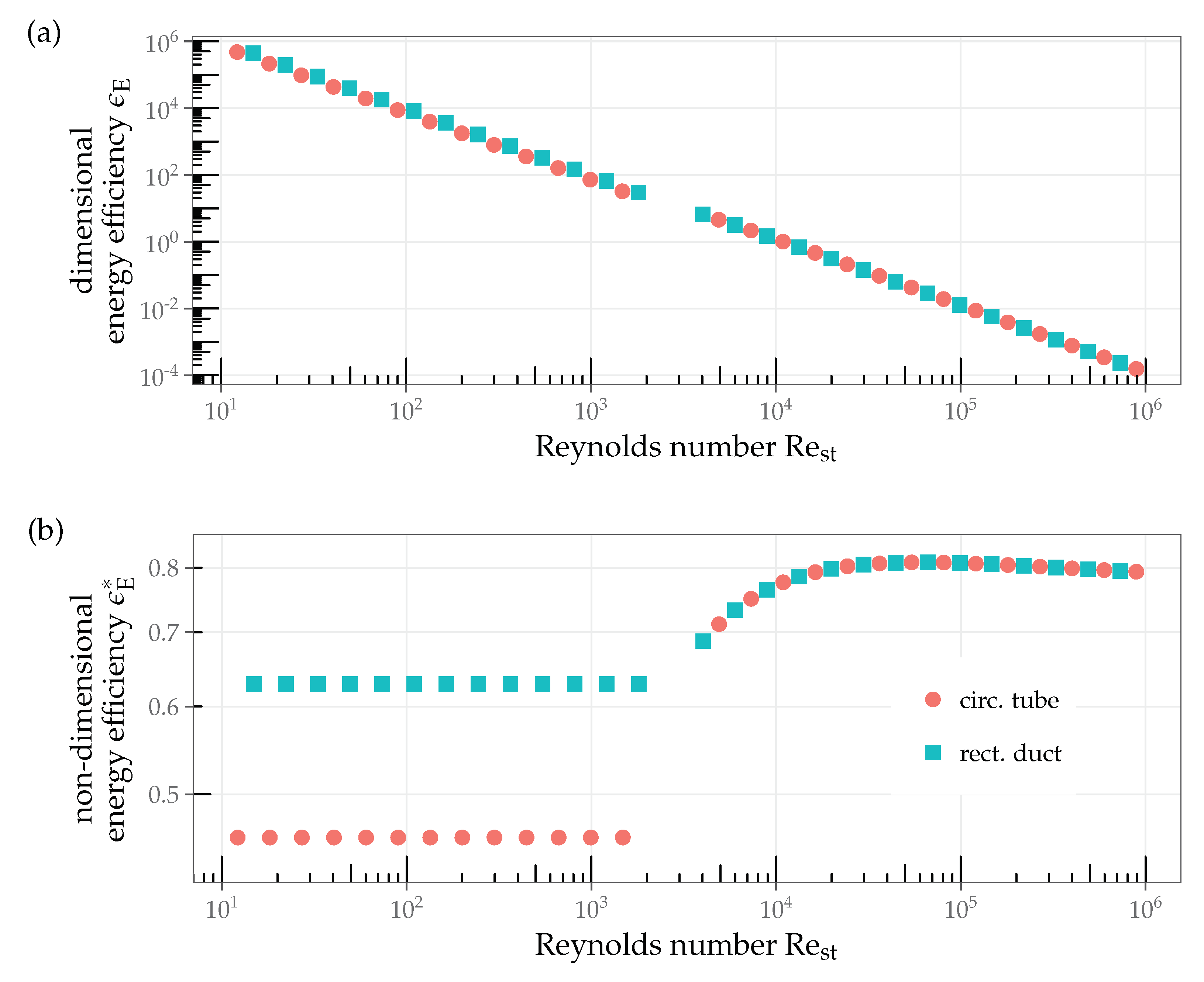
2.1.1. Definition of Dimensional Evaluation Criteria
2.1.2. Definition of Non-Dimensional Evaluation Criteria
- the generation of the non-dimensional efficiencies is independent of the restrictions (1) to (5)
- a comparison of non-dimensional efficiencies of different heat transfer surface enhancements is based on the restrictions (1) to (5)
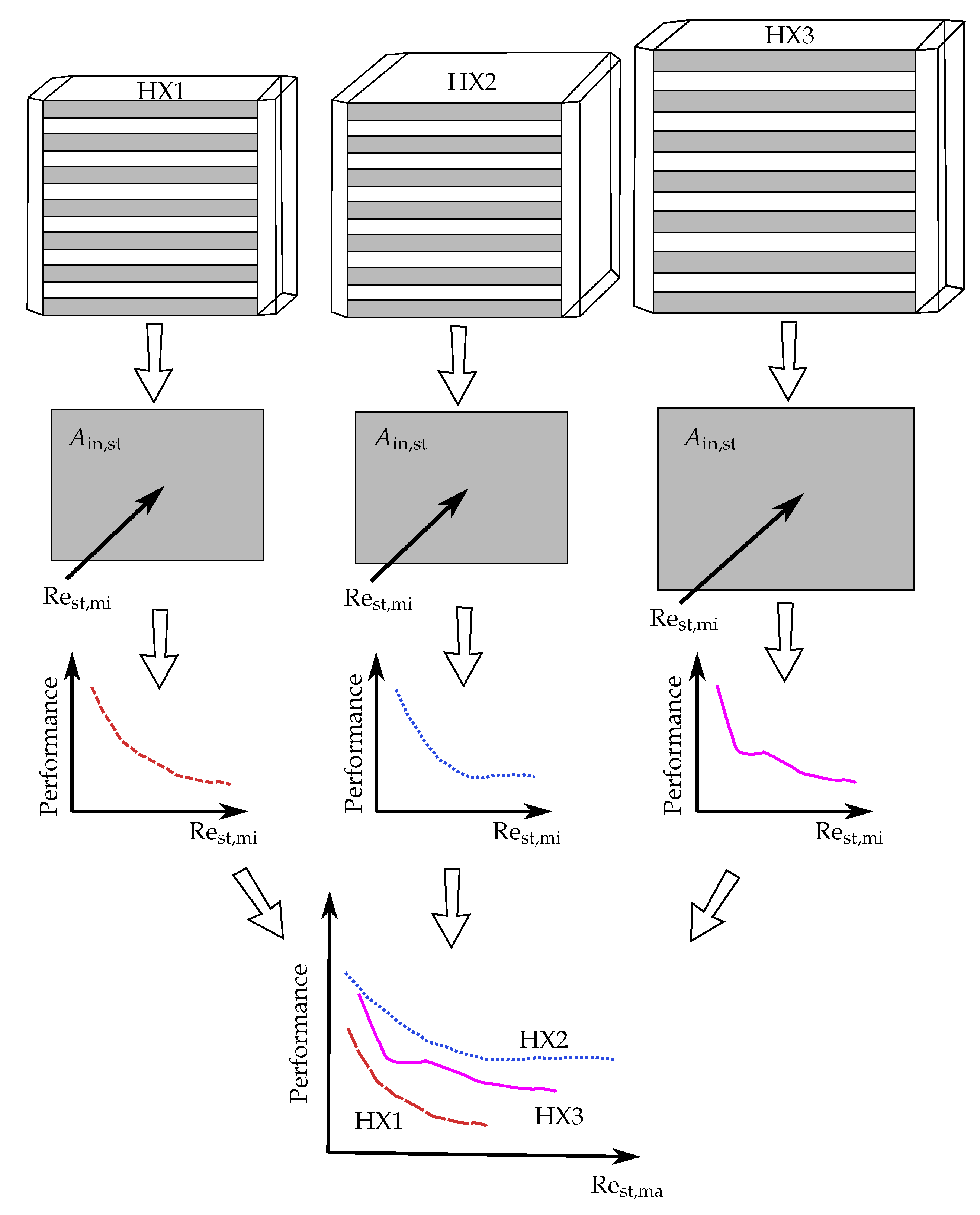
- Two equal heat exchangers arranged either in parallel or in-line are on the same efficiency curve as only one of these heat exchangers.
- When the geometric dimension of a heat exchanger is scaled (e.g., from large to small) the efficiency curve keeps its shape but experiences a stretching (e.g., to the right) along the x-axis.
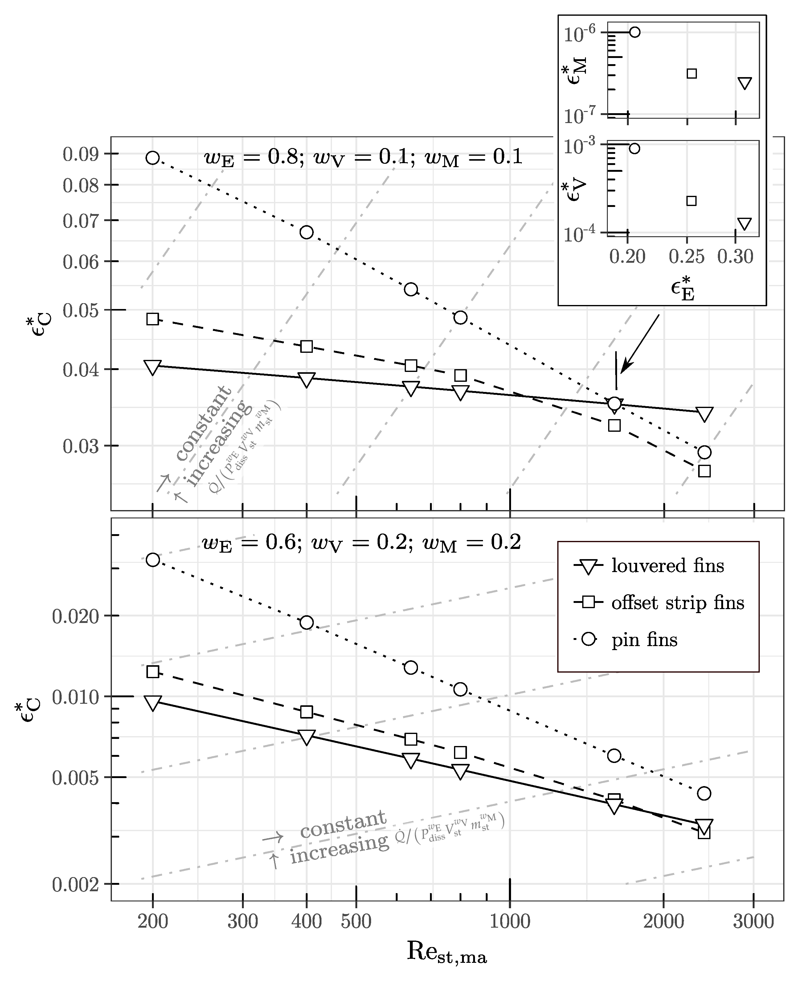
2.2. Scalarizing of Multi-Objective Optimization Problems
3. Results
4. Discussion
5. Conclusions
- Development of a dimensional performance evaluation method including energy, volume, and mass, allowing straightforward transfer to important quantities for real dimensioning,
- Transformation of dimensional performance evaluation quantities into non-dimensional quantities (efficiencies) based on comparable driving parameters,
- Application of the performance evaluation method to optimize a surface enhancement geometry (topology) or to compare different surface enhancements with each other,
- Control of energy, volume, and mass use for the optimization/comparison by setting the efficiencies as objective functions,
- Usage of thermal-hydraulic correlations from the literature, measurement data, or simulation data within the performance evaluation method,
- Development of a combined efficiency for single-objective optimization,
- Non-dimensional performance evaluation quantities are independent of characteristic lengths
Author Contributions
Funding
Conflicts of Interest
Abbreviations
| A | surface area |
| heat transfer surface area of the primary and secondary surfaces on the air-side | |
| free-flow area at the inlet of the structure volume | |
| heat transfer surface area of the secondary structure surface on the air-side | |
| Brinkman number (Equation (10)) | |
| specific heat | |
| d | characteristic diameter |
| characteristic macro-scale diameter for heat exchanger | |
| characteristic micro-scale diameter for structure | |
| characteristic diameter for the structure (equals for the wire structure) | |
| f | friction factor |
| Fanning friction factor (Equation (4)) | |
| G | fluid mass velocity based on the free-flow area |
| height of the structure | |
| h | convective heat transfer coefficient |
| air-side convective heat transfer coefficient based on the surface area | |
| j | Colburn factor |
| contraction loss coefficient | |
| exit loss coefficient | |
| mean thermal conductivity of air within the structure | |
| thermal conductivity of the solid material used for the structure | |
| length of the structure | |
| l | length of fin ([5], p. 289) |
| lateral distance (pitch) of the wires or fins | |
| longitudinal distance of the wires | |
| m | auxiliary coefficient for fin efficiency ([5], p. 289) |
| mass flow rate of air | |
| mass of the structure | |
| Nusselt number (Equation (3)) | |
| p | pressure |
| dissipated power | |
| Prandtl number | |
| heat transfer rate | |
| Re | Reynolds number |
| Reynolds number (Equation (2)) | |
| Reynolds number based on and specified | |
| Reynolds number based on and specified | |
| T | temperature |
| inlet temperature | |
| U | overall heat transfer coefficient |
| V | volume |
| available volume for structure between the tubes or plates | |
| volume of the solid part of a structure without the air volume | |
| superficial structure air velocity based on and | |
| volume flow rate based on and | |
| Greek Symbols | |
| heat transfer surface area density (Equation (5)) | |
| temperature difference between the air inlet and outlet | |
| mean temperature difference between two domains | |
| pressure drop associated with a heat exchanger | |
| pressure drop within the core structure | |
| dimensional efficiency | |
| non-dimensional efficiency | |
| mean kinematic air viscosity within the structure | |
| fin efficiency | |
| extended surface efficiency | |
| mean air density within the structure | |
| density of the solid material used for structure | |
| porosity of the structure (Equation (6)) | |
| ratio of the thermal conductivity of the structure versus that of the air | |
| Subscripts | |
| E | energy-specific |
| HX | heat exchanger |
| M | mass-specific |
| PEC | performance evaluation criteria |
| st | structure |
| std | standard |
| V | volume-specific |
Appendix A. Pressure Drop Calculation
Appendix B. Transformation from Dimensional to Non-Dimensional Key Figures
Appendix C. Fin Efficiency
Appendix D. Dependencies

| Parameter | Dependency | Source | Comment |
|---|---|---|---|
| , , , geometry | ([23], ch. 3), ([24], p. 523) | T in Kelvin; influence of for gases is usually small | |
| , geometry | ([5], ch. 6) | Risk of confusion between Darcy and Fanning friction factor | |
| , , , geometry | ([5], p. 289) | Simplified assumptions on geometry are used |
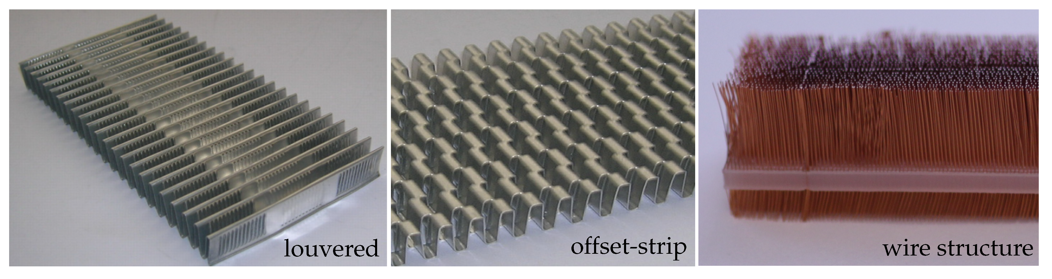
Appendix E. Exemplary Heat Transfer Enhancements
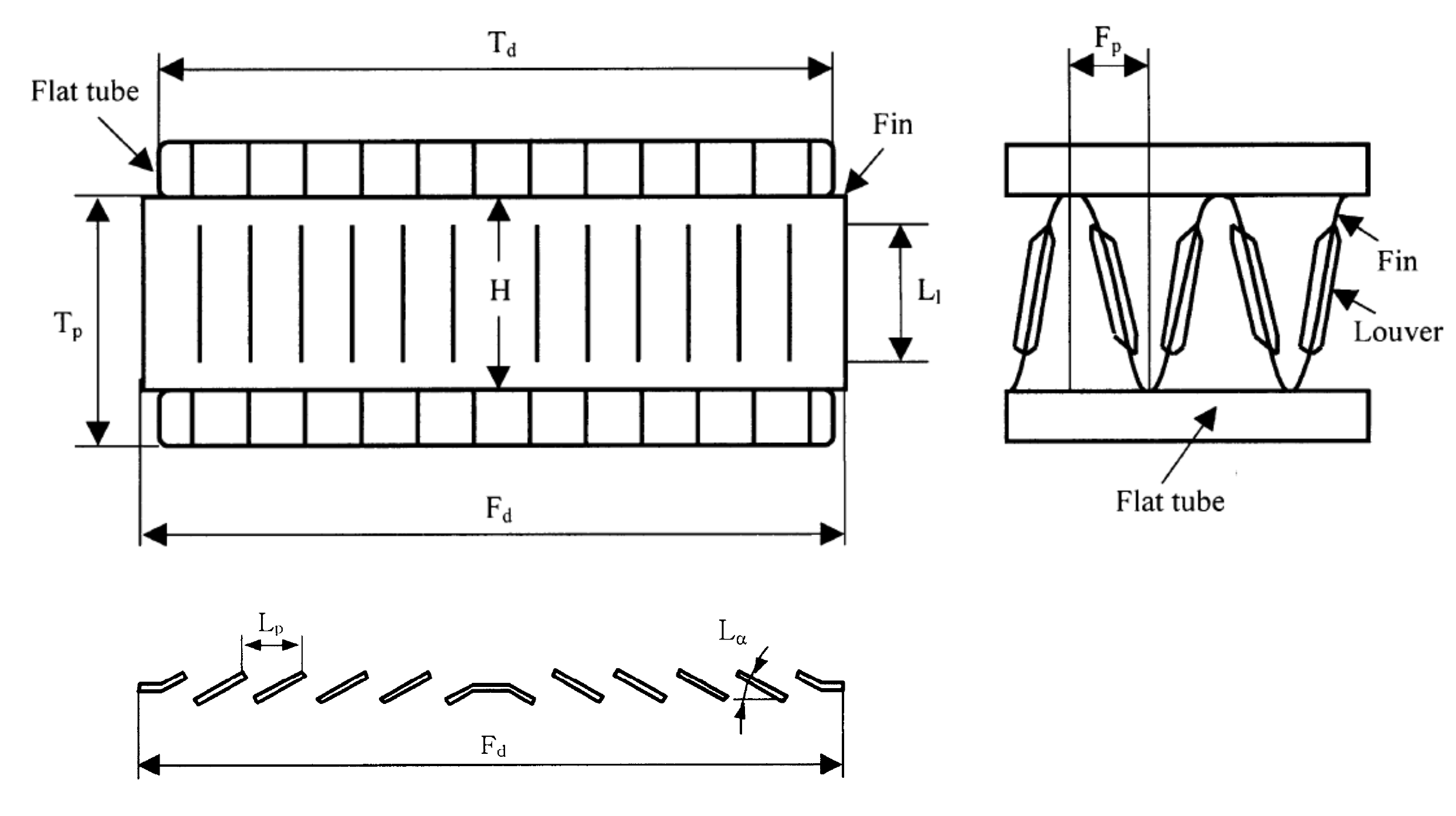
Appendix E.1. Louvered Fins
Appendix E.2. Offset Strip Fins
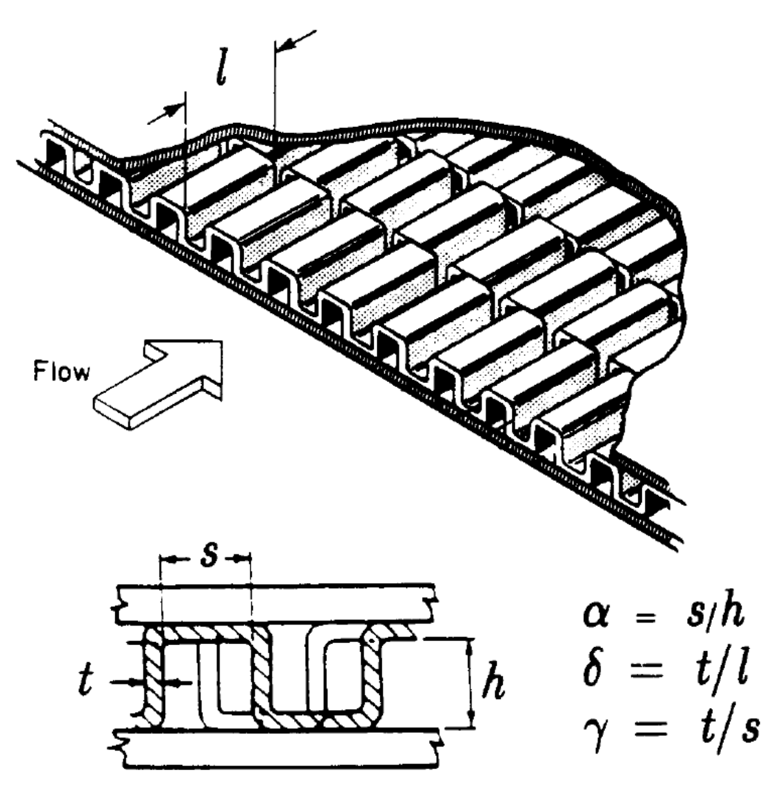
Appendix E.3. Wire Structure Pin Fins

References
- Stone, K.M. Review of Literature on Heat Transfer Enhancement in Compact Heat Exchangers; Air Conditioning & Refrigeration Center: Urbana, IL, USA, 1996. [Google Scholar]
- Fugmann, H.; Laurenz, E.; Schnabel, L. Wire Structure Heat Exchangers—New Designs for Efficient Heat Transfer. Energies 2017, 10, 1341. [Google Scholar] [CrossRef]
- LaHaye, P.G.; Neugebauer, F.J.; Sakhuja, R.K. A Generalized Prediction of Heat Transfer Surfaces. J. Heat Transf. 1974, 96, 511. [Google Scholar] [CrossRef]
- Webb, R.L. Goodness Factor Comparisons. In HEDH Multimedia; Begellhouse: Danbury, CT, USA, 2014. [Google Scholar] [CrossRef]
- Shah, R.K.; Sekulić, D.P. Fundamentals of Heat Exchanger Design, 1st ed.; John Wiley & Sons: Hoboken, NJ, USA, 2003. [Google Scholar]
- Webb, R.L.; Kim, N.H. Principle of Enhanced Heat Transfer; Taylor & Francis: Abingdon, UK, 1994. [Google Scholar]
- Soland, J.G. Performance Ranking of Plate-Finned Heat Exchanger Surfaces. Ph.D Thesis, Massachusetts Institute of Technology, Cambridge, MA, USA, 1975. [Google Scholar]
- Cowell, T.A. Comparison of Compact Heat Transfer Surfaces. J. Heat Transf. 1990, 112, 288–294. [Google Scholar] [CrossRef]
- Sahiti, N.; Durst, F.; Dewan, A. Strategy for selection of elements for heat transfer enhancement. Int. J. Heat Mass Transf. 2006, 49, 3392–3400. [Google Scholar] [CrossRef]
- Li, Q.; Flamant, G.; Yuan, X.; Neveu, P.; Luo, L. Compact heat exchangers: A review and future applications for a new generation of high temperature solar receivers. Renew. Sustain. Energy Rev. 2011, 15, 4855–4875. [Google Scholar] [CrossRef]
- Marthinuss, J.E. Air Cooled Compact Heat Exchanger Design For Electronics Cooling. Coolers Design Heat Sinks Test Measur. 2004, 10, 28. [Google Scholar]
- Korhonen, P.; Wallenius, J. Visualization. In Multiple Objective Decision-Making Framework; Springer: Berlin, Germany, 2008. [Google Scholar]
- Miettinen, K.; Mäkelä, M.M. On scalarizing functions in multiobjective optimization. OR Spectr. 2001, 24, 193–213. [Google Scholar] [CrossRef]
- Triantaphyllou, E.; Parlos, P.M. Multi-Criteria Decision Making Methods: A Comparative Study. In Applied Optimization; Kluwer Academic Publishers: Dordrecht, The Netherlands, 2010; Volume 44. [Google Scholar]
- Kim, M.H.; Bullard, C.W. Air-side thermal hydraulic performance of multi-louvered fin aluminum heat exchangers. Int. J. Refrig. 2002, 25, 390–400. [Google Scholar] [CrossRef]
- Manglik, R.M.; Bergles, A.E. Heat transfer and pressure drop correlations for the rectangular offset strip fin compact heat exchanger. Exp. Therm. Fluid Sci. 1995, 10, 171–180, Figures reprinted with permission from Elsevier. [Google Scholar] [CrossRef]
- Fugmann, H.; Schnabel, L.; Frohnapfel, B. Heat Transfer and Pressure Drop Correlations for Laminar Flow in an In-line and Staggered Array of Circular Cylinders. Numer. Heat Transf. Part A Appl. 2019, 75, 1–20. [Google Scholar] [CrossRef]
- Fugmann, H.; Di Lauro, P.; Sawant, A.; Schnabel, L. Development of Heat Transfer Surface Area Enhancements: A Test Facility for New Heat Exchanger Designs. Energies 2018, 11, 1322. [Google Scholar] [CrossRef]
- Dong, J.; Chen, J.; Chen, Z.; Zhang, W.; Zhou, Y. Heat transfer and pressure drop correlations for the multi-louvered fin compact heat exchangers. Energy Convers. Manag. 2007, 48, 1506–1515, Figures reprinted with permission from Elsevier. [Google Scholar] [CrossRef]
- Dong, J.; Chen, J.; Chen, Z.; Zhou, Y. Air-side thermal hydraulic performance of offset strip fin aluminum heat exchangers. Appl. Therm. Eng. 2007, 27, 306–313. [Google Scholar] [CrossRef]
- Mahulikar, S.P.; Herwig, H. Fluid friction in incompressible laminar convection: Reynolds’ analogy revisited for variable fluid properties. Eur. Phys. J. B 2008, 62, 77–86. [Google Scholar] [CrossRef]
- MIT. The Reynolds Analogy. 2019. Available online: web.mit.edu.
- Böckh, P.; Wetzel, T. Wärmeübertragung: Grundlagen und Praxis, Aktualisierte und Überarbeitete Auflage ed.; Lehrbuch Springer Vieweg: Berlin, Germany, 2017. [Google Scholar]
- Verein Deutscher Ingenieure. Wärmeatlas, 9th ed.; Springer: Berlin/Heidelberg, Germany, 2002. [Google Scholar]


| Method | Sources | Assets | Inclusion of Conductivity of Fins |
|---|---|---|---|
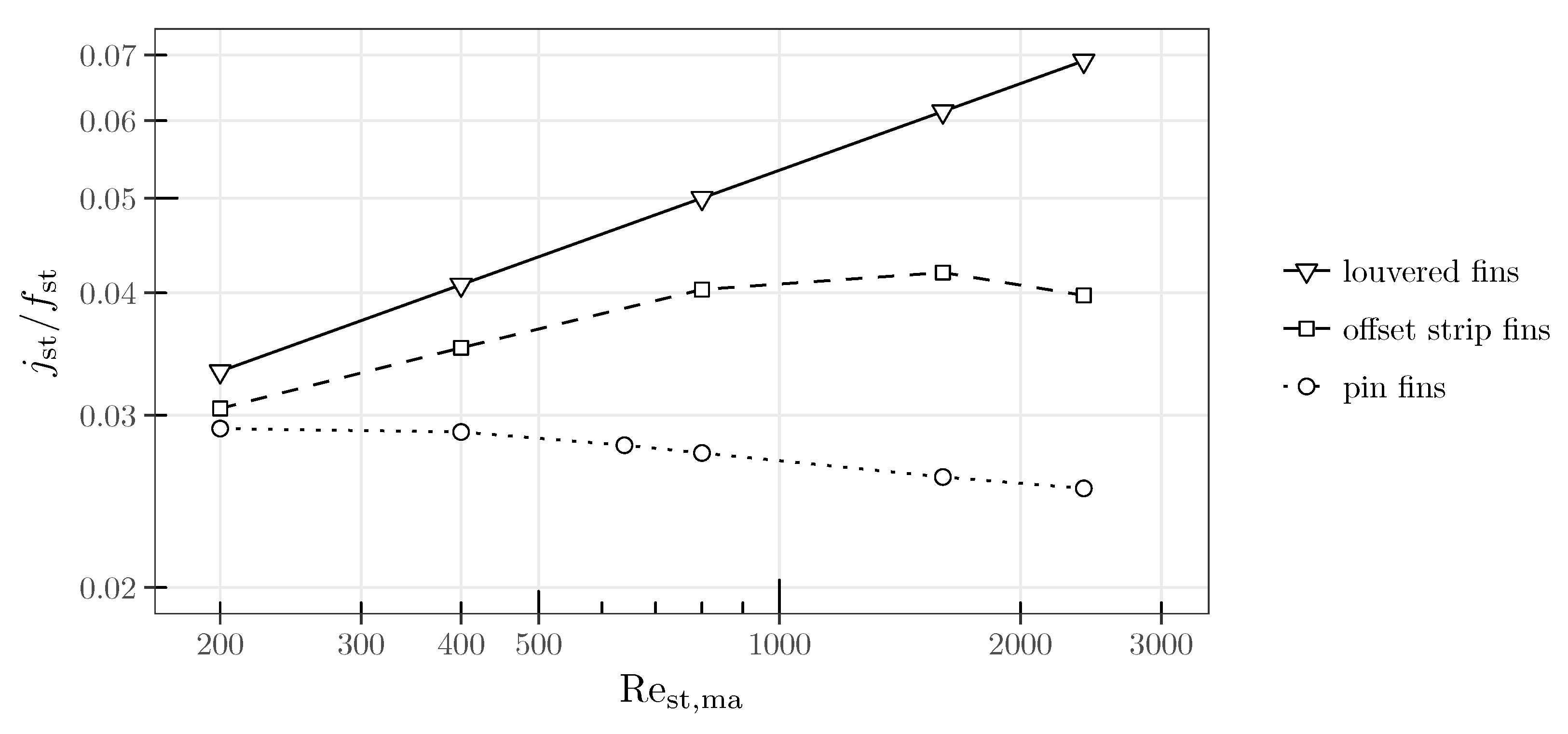
| j and f vs. curves | [1,3] | simple visualization of the thermal-hydraulic performance | no |
| Area goodness factor | [1,5] | identification of feasible surfaces with low free-flow area | no |
| Volume goodness factor | [5] | identification of feasible surfaces with low volume | yes |
| Performance evaluation criteria (PEC) | [5,6] | designer-specific choice of evaluation criteria | (yes) * |
| Performance parameters | [1,3] | convenient method for comparing various heat transfer geometries in one figure | no |
| Ranking performance | [7] | comparison of very different fin types with respect to different designer conditions | no |
| General comparison method | [8] | designer-specific choice of evaluation criteria | no |
| Energetic comparison | [9] | no volume or surface geometry constraints | yes |
| Cost | Key Figure | Main Definition | Alternative Definition | Dimension |
|---|---|---|---|---|
| Dissipated power on the air-side in , which is proportional to the electric power consumption of the fans | Energy efficiency | 1/ | ||
| Available volume for heat transfer enhancement in (excluding fluid guidance volume and header/distributor) | Volume efficiency | |||
| Material usage for the wire or fin structure in kg (excluding fluid guidance, solder material and header/distributor) | Mass efficiency | /() |
| Description | Key Figure | Definition | Relation to Dimensional Parameter | Reduced Expression |
|---|---|---|---|---|
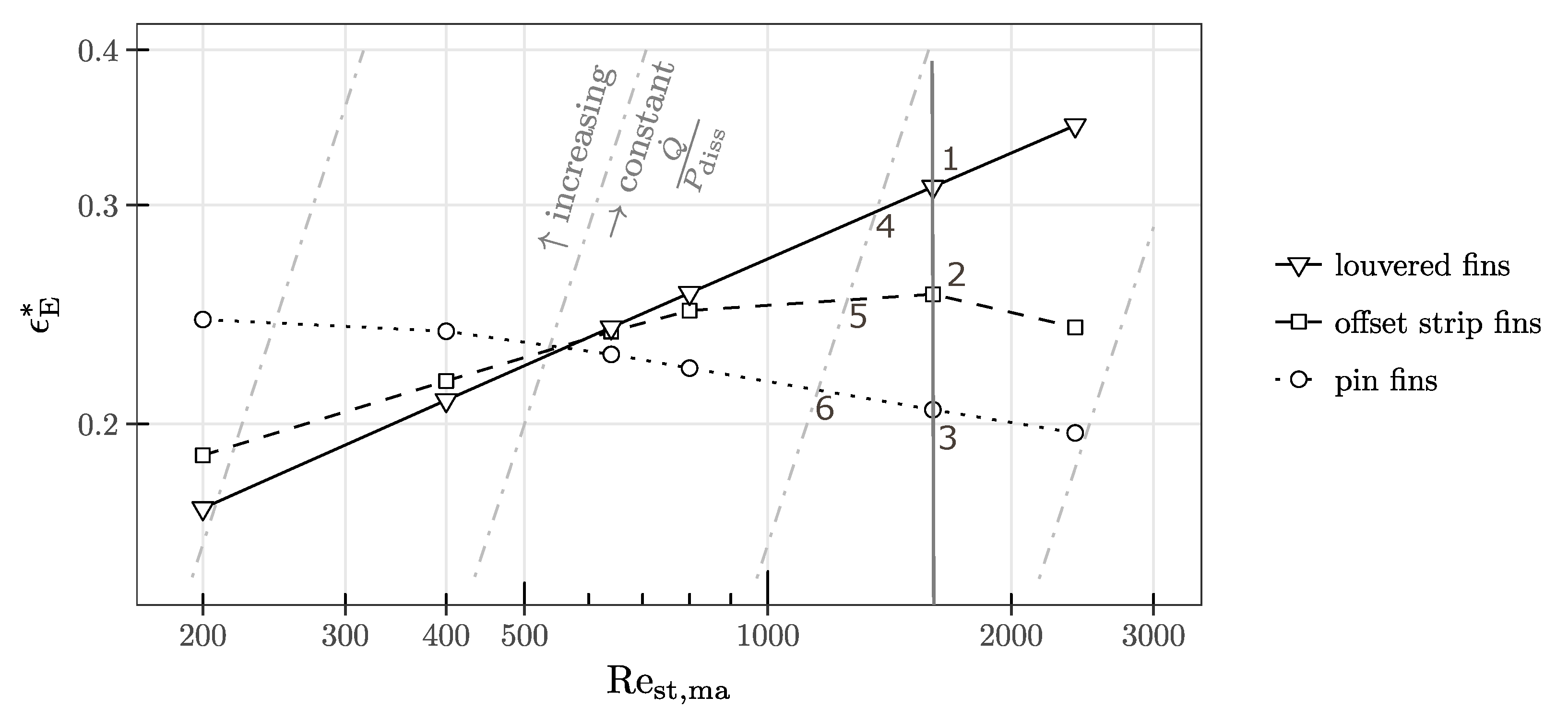
| Energy efficiency | ||||
| Volume efficiency | ||||
| Mass efficiency |
| Parameter | Dimension | Louvered Fin | Offset Strip Fin | Wire Structure |
|---|---|---|---|---|
| Source | ‒ | [15] | [16] | [17,18] |
| Thermal conductivity structure, | W/(mK) | 385 | 385 | 385 |
| Fin pitch, | mm | 2.3 | 1.9 | 1.2 |
| Substructure length, | mm | 4.76 | 1.01 | 0.35 |
| Structure thickness, | μm | 152 | 152 | 250 |
| Structure length, | mm | 48 | ‒ | 10 |
| Structure height, | mm | 10 | 10 | 10 |
| Heat transfer surface area density, | / | 1083 | 1403 | 2024 |
| Porosity, | ‒ | 0.93 | 0.91 | 0.88 |
| Micro-diameter, | mm | 4.76 | 2.58 | 0.25 |
| Macro-diameter, | mm | 10 | 10 | 10 |
© 2019 by the authors. Licensee MDPI, Basel, Switzerland. This article is an open access article distributed under the terms and conditions of the Creative Commons Attribution (CC BY) license (http://creativecommons.org/licenses/by/4.0/).
Share and Cite
Fugmann, H.; Laurenz, E.; Schnabel, L. Multi-Dimensional Performance Evaluation of Heat Exchanger Surface Enhancements. Energies 2019, 12, 1406. https://doi.org/10.3390/en12071406
Fugmann H, Laurenz E, Schnabel L. Multi-Dimensional Performance Evaluation of Heat Exchanger Surface Enhancements. Energies. 2019; 12(7):1406. https://doi.org/10.3390/en12071406
Chicago/Turabian StyleFugmann, Hannes, Eric Laurenz, and Lena Schnabel. 2019. "Multi-Dimensional Performance Evaluation of Heat Exchanger Surface Enhancements" Energies 12, no. 7: 1406. https://doi.org/10.3390/en12071406
APA StyleFugmann, H., Laurenz, E., & Schnabel, L. (2019). Multi-Dimensional Performance Evaluation of Heat Exchanger Surface Enhancements. Energies, 12(7), 1406. https://doi.org/10.3390/en12071406