Including Wind Power Generation in Brazil’s Long-Term Optimization Model for Energy Planning

Abstract

In the past two decades, wind power’s share of the energy mix has grown significantly in Brazil. However, nowadays planning electricity operation in Brazil basically involves evaluating the future conditions of energy supply from hydro and thermal sources over the planning horizon. In this context, wind power sources are not stochastically treated. This work applies an innovative approach that incorporates wind power generation in the Brazilian hydro-thermal dispatch using the analytical method of Frequency & Duration. The proposed approach is applied to Brazil’s Northeast region, covering the planning period from July 2017 to December 2021, using the Markov chain Monte Carlo method to simulate wind power scenarios. The obtained results are more conservative than the one currently used by the National Electric System Operator, since the proposed approach forecasts 1.8% less wind generation, especially during peak periods, and 0.67% more thermal generation. This conservatism can reduce the chance of water reservoir depletion and, also an ineffective dispatch.

1. Introduction

The depletion of traditional energy sources, such as water and fossil fuels, as well as concerns about the sustainability, safety and reliability of energy supply systems, has caused intense growth of wind power generation worldwide. In Brazil, in the last two decades wind energy share in the e energy mix has grown significantly, reaching 8.1% (13 GW) of installed capacity in July 2018, with 536 projects in operation [1]. Official expectations for 2026 indicate an increase of approximately 215%, reaching 28 GW of installed capacity [2] and another 229 enterprises in operation. Regarding the participation in the energy generation, in March 2006 wind power was responsible for only 0.075 GWh, 0.002% of the total generation, while in September 2017 this figure reached 5 TWh, representing 11% of the country’s electricity generation that month.

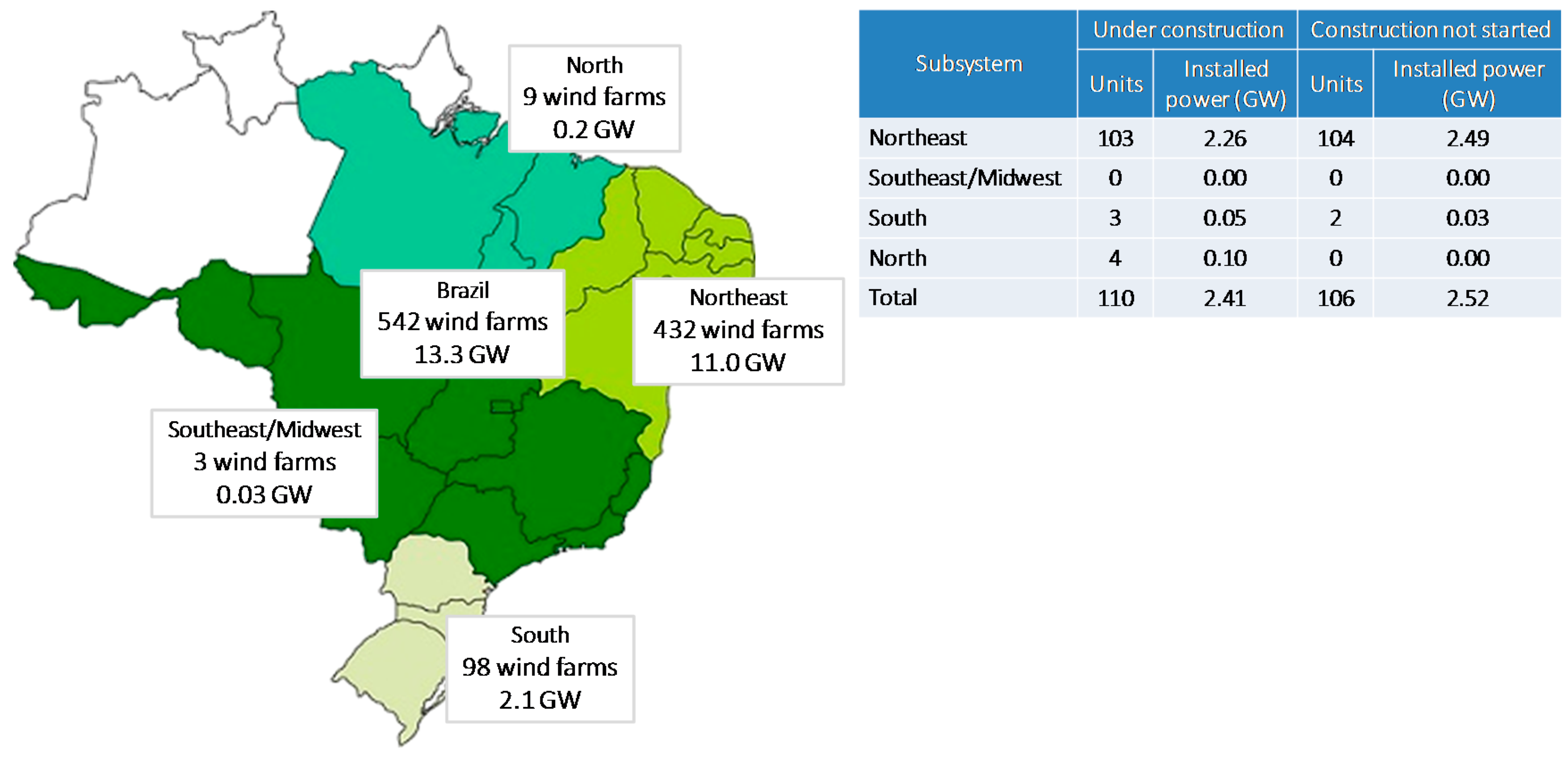
Since Brazil is a country with continental dimensions, the Brazilian electricity sector (BES) is divided into four interconnected submarkets, corresponding to the country’s geographic regions: North, Northeast, South and Southeast/Midwest. Figure 1 shows the high concentration (80%) of wind farms in the Northeast, a consequence of the presence of strong winds in the region and the complementarity between wind and water sources [3], in contrast to what happens in the Southeast/Midwest, which has only 0.55% of the projects. Most of the plants already under construction or planned for construction are also located in the Northeast, totaling 207 new ventures in the region of the 216 nationwide.

Despite the increase of wind power generation, the Brazilian electrical system is basically formed by hydroelectric and thermal plants, which together represented approximately 70% of the country’s total generation in 2017 [4,5,6]. Nowadays, planning the BES operation basically involves evaluating the future conditions of energy supply from hydro and thermal sources over the planning horizon to minimize the expected value of the operation cost during the planning period [7,8,9]. This cost is formed by the fuel costs plus penalties for failure of load supply, under operational and security constraints [10,11,12]. The other generation sources, including wind power, are discounted from energy demand in a deterministic way. That is, the current dispatch model does not consider wind generation’s stochastic behavior. Suomalainen et al. [13] showed that in a system highly influenced by seasonal hydraulic generation, the high penetration of wind sources causes large impacts on the dispatch models. This is because wind generation mainly depends, on wind speed, a renewable and abundant resource, but one that is volatile. From an operational perspective, this volatility is a disadvantage, considering that for hydroelectric generation it is possible to minimize this variation through reservoir management [14].

In order to model the wind data at a particular site, an extensive historical series is necessary. If these datasets are not available, stochastic simulation techniques are required. The first important work dealing with simulation of wind speed data was published in 1996 and used statistical tests to check the adequacy of an autoregressive moving average (ARMA) model to provide this simulation [15]. Castino et al. [16] applied Markov chain and discrete autoregressive models to forecast wind series using information on wind speed and direction. Alexiadis et al. [17] predicted wind speed and power via artificial neural networks (ANN) and autoregressive models, showing that the first presents better accuracy. Papaefthymiou and Klöckl [18] presented a Markov chain Monte Carlo (MCMC) approach for the direct generation of synthetic time series of wind power output. Pinson [19] emphasized the importance of considering wind power generation as a stochastic process, and Zhang et al. [20] proved that wind power generation can be modeled as a stochastic process, since it is both nonlinear and unstable. Jung and Broadwater [21] presented a literature review of wind speed and power forecasting, involving spatial, probabilistic and offshore correlation, showing that the formulations cannot be compared since each model depends on the location (spatial correlation). Iversen et al. [22] proposed a modeling framework for wind speed based on stochastic differential equations. Landry et al. [23] described the probabilistic wind power forecasting method that was used to win the wind track of the Global Energy Forecasting Competition in 2014 (GEFCom2014). Aguilar et al. [24] developed a hybrid methodology using Singular Spectrum Analysis (SSA) and Conditional Kernel Density Estimation to achieve accurate probabilistic forecasts of wind output, and Cheng et al. [25] proposed an ensemble model for probabilistic wind speed forecasting. Ekström et al. [26] presented an improved method for the detailed statistical modeling of wind power generation based on a vector autoregressive model.

Besides wind generation, modeling and forecasting, this work aims to integrate these results in the current hydro-thermal dispatch model, without the need of any structural change in the optimization model, by updating the calculation of the non-dispatched plants. In order to reach the proposed objective and to consider the wind time series’ stochastic behavior, the Frequency and Duration (F&D) methodological principle is used, combining via Markov chain Monte Carlo method the states of generation and load capacity to determine those ones of net demand and the corresponding probabilities. The F&D method is widely used to evaluate the static capacity adequacy for a given generation system, with the first application dating from 1968 [27]. This paper is based on the method developed by Leite da Silva et al. [28], which represents generation units by multistate models and load by hourly data. It also shows that not only the availability of the reserve states can be evaluated by discrete convolution, but also their frequencies. The methodology proposed here can be applied to other countries that face similar problems, that is, expanding reliance on intermittent sources while complementing the main sources, in addition to a centralized long-term operational planning without the possibility of modifying the equations of the optimization model, as, for example, Chile [29] and Nordic countries [30]. The Climate Forecast System Reanalysis combined with technical turbine information was used to obtain the historical time series from each wind farm, detailed in Section 3.1. All the statistical analysis and simulations were developed in R Statistical Software [31]. The optimization model was developed by the Stochastic Dual Dynamic Programming (SDDP) model [32]. In this sense, the novelty of this paper is the inclusion, via a stochastic approach, of the wind power generation into the optimal operation of the hydrothermal Brazilian system, resulting in the so called wind-hydro-thermal dispatch. Given that the wind power penetration is rather new in Brazil and is growing very fast, the lack of historical data is a real technical challenge for the implementation of such procedure.

The remainder of this paper is organized as follows: Section 2 presents a step-by-step framework to reach the goals described previously. Section 3 describes the results obtained, comparing our scenarios and the real datasets, as well as the wind power calibration outcome, and, finally the net demand calculation. Section 4 provides conclusions and future research directions.

2. Material and Methods

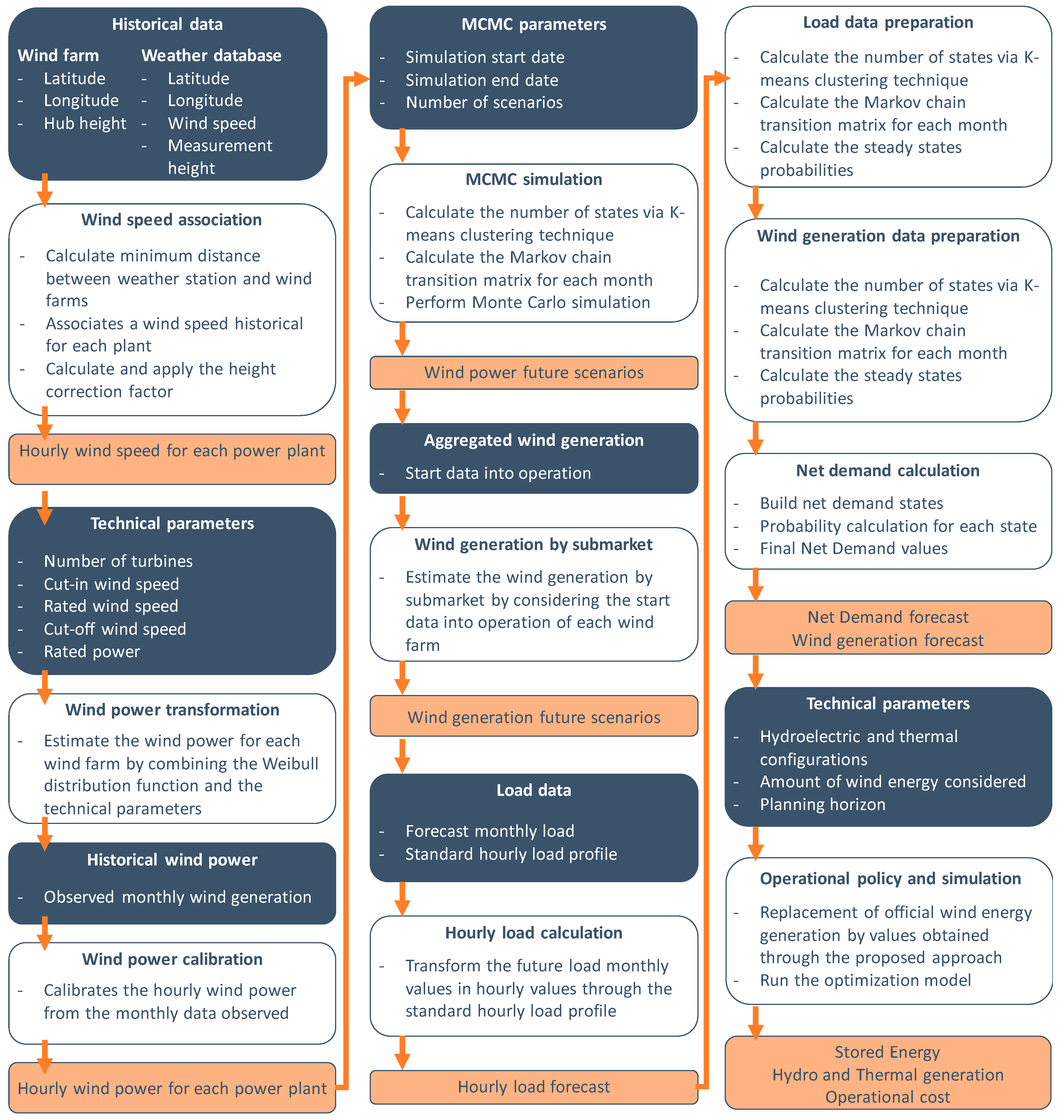
The introduction section emphasizes the growing trend of wind power generation in the Brazilian electricity mix and the need to consider the stochastic behavior of this source in the electric operation planning model. To meet this need, we propose a methodology that can be divided into three dependent procedures: historical measurements, Markov chain Monte Carlo (MCMC) modeling and the net demand approach.

Figure 2 presents a graphical framework with a description of all the calculations. In the first stage, each plant is associated with a wind speed history, obtained through measurements stations, and that speed is converted into wind power through the combination of turbine technical parameters. The data are calibrated from observed wind generation values. In the second stage, future scenarios of wind generation for each power plant are simulated using the Markov chain Monte Carlo method. In order to build the wind power generation of an entire submarket, the start-up date of each plant is considered. In the third stage, the expected energy load is considered with hourly frequency, being constructed through load profiles and future values. The calculation of the net demand is done through the combination of possible states of energy load and wind generation and probabilities are associated with each state. After obtaining the expected values of wind generation and net demand, it is necessary to include these data in the Brazilian hydro-thermal dispatch by replacing the wind energy values considered by the BES with the values obtained through the proposed approach. Such dispatch is based on an optimization model, where the income inflow is the stochastic variable. The objective function intends to minimize the sum of immediate and future cost of fuel and energy deficit, under operational and security constraints. The future cost is a convex combination of the expected value of the future cost function and the Conditional Value at Risk (CVaR) of that function, in order to insert risk aversion [33].

It should be noted that there are other solutions for the inclusion of wind energy, and other so-called intermittent sources, directly in the dispatch optimization. Examples are the work of Papavasiliou et al. [34], who developed the multistage stochastic programming formulation; Jurasz et al. [35], who developed a mixed-integer nonlinear mathematical model; Morillo et al. [36], who included the expected production of wind energy in the objective function; and Raby et al. [29], who considered wind power as a new thermal plant. However, one of the main objectives of this work is to propose an approach that considers the variability of the wind series, but does not change the optimization model’s formulation.

2.1. Historical Measurements

In the proposed methodology the first stage is related to the historical measurements, where the first step consists of obtaining a full year history of hourly wind speed series at the selected location. This information can be accessed through the Climate Forecast System Reanalysis (CFSR) [37] maintained by the National Centers for Environmental Prediction (NCEP). Through the CFSR it is possible to obtain the desired information according to geographic coordinates, with a spatial resolution of 0.25° by 0.25°. Thus, the association of a wind speed series to a wind farm was carried out by searching for the measurement point that minimizes the distance between them.

As a consequence of the difference in height between the measurement of wind speed (10 m) and the height of the turbines, it is necessary to consider a height correction factor [38], given that the greater the height the greater the wind speed generally it. This can be calculated by the natural logarithm ratio of the turbine height and the point at which wind measurement is performed, as in Equation (1):

$$H{F}_i=\frac{\log \left(H{T}_i\right)}{\log \left(H{M}_i\right)}$$

(1)

where $H{F}_i$ is the height correction factor, $H{T}_i$ is the turbine height and $H{M}_i$ is the measurement height associated with wind farm $i$. So, the final wind speed, $W{S}_{h,d,m,i}$, associated with the wind farms is the result of multiplying the height correction factor by the original wind speed, $OW{S}_{h,d,m,i}$:

$$W{S}_{h,d,m,i}=H{F}_i\times OW{S}_{h,d,m,i}$$

(2)

where $h$ is the hour, $d$ is the day and $m$ is the month.

According to Papaefthymiou and Klöckl [18], simulated wind power is more adequate than wind speed. There are two reasons for this (i) it avoids errors calculations in the conversion of speed to power; and (ii) the number of states is smaller, since the wind power is only observed for a given range of wind speed values. So, here we use the wind power series to simulate the future wind generation.

A convenient way to obtain the output power of a given wind turbine is through its power curve, which relates the resulting power of the turbine to a specific wind speed. Turbine manufacturers provide the power curves in tabular or graphic form. However, a generic equation that accurately represents this curve is needed in many problems involving wind power. The work of Kusiak et al. [39] identified that proper selection of power curve models is essential for predicting power and online monitoring of turbines accurately. Such models can be classified as discrete, deterministic/probabilistic, parametric/nonparametric and stochastic. Sohoni et al. [40] present a literature review of the existing methods for approximation of the power curve and the advantages and disadvantages involved in each one.

A parametric model defines the relation between input and output through a set of mathematical equations with a finite number of parameters. The transformation of wind speed into wind power ($WP{A}_{h,d,m,i}$) is made by a parametric model of the power curve of wind turbine expressed in Equation (3):

$$WP{A}_{h,d,m,i}=\{\begin{array}{c}0\\ q\left(v\right)\\ P_r\end{array}\begin{array}{c}W{S}_{h,d,m,i}\langle v_{ci},W{S}_{h,d,m,i}\rangle v_{co}\\ v_{ci}<W{S}_{h,d,m,i}<v_r\\ v_r\le W{S}_{h,d,m,i}\le v_{co}\end{array}$$

(3)

where $v_{ci}$ is the initial velocity at which wind starts generating power, and $v_r$ is the cutting velocity, starting from which to the final velocity $v_{co}$, the power generated will be the same and equal to the rated power $P_r$ of the turbine. For any velocity less than the initial one $v_{ci}$ and greater than the final velocity $v_{co}$, there is no power generated. The relation between the resulting power and the wind speed between the initial velocity ($v_{ci}$) and the cutting velocity ($v_r$) is nonlinear and is represented by $q\left(v\right)$ in Equation (3). However, this relation can be approximated by different functions, polynomial or not. In this work, we selected the method based on the Weibull distribution (Equation (4)) [41,42], where the parameter $k$ is the shape and is obtained by adjusting the maximum likelihood of the Weibull distribution function to the wind speed data from each month.

$$q\left(v\right)=\left(\frac{v_{ci}^{k_m}}{v_{ci}^{k_m}-v_r^{k_m}}+\frac{{{WS}_{h,d,m,i}}^{k_m}}{v_{co}^{k_m}-v_{ci}^{k_m}}\right)P_r$$

(4)

So far, all the wind speed considered is converted into wind power ($WP{A}_{h,d,m,i}$), considering the turbine capacity factor. In this sense, the calibration year was the one when the data were obtained. That is, the calibration factor will be calculated from the observed monthly wind generation values and also the calculated monthly wind generation values, as in Equation 5, where $W{P}_{h,d,m,i}$ is the calibrated wind power, $WP{A}_{m,i}$ is the total wind power calculated for month $m$ and wind farm $i$ and $O_{m,i}$ is the observed wind generation at month $m$ and wind farm $i$:

$$W{P}_{h,d,m,i}=WP{A}_{h,d,m,i}\times \frac{O_{m,i}}{W{P}_{m,i}}$$

(5)

2.2. Stochastic Wind Power Simulation

The procedure developed in this study to stochastically simulate the wind power data is based on Almutairi et al. [43]. The first step involves the application of the K-means clustering technique [44] to transform the wind power data $\left(W{P}_{h,d,m,i}\right)$ into a finite number of states $\left(WP{S}_{h,d,m,i}\right)$. For the K-means technique, given a number $k$ of clusters and $M_k$ initial centroids, the distance $D_{k,c}$ from each wind power value $W{P}_c$ to each $M_c$ is calculated and all of the wind power values are assigned to the nearest centroid. New cluster centroids are calculated using the average of the wind power data in cluster $k$ and the distances are recalculated. This process is repeated until the centroids remain fixed after a number of iterations. At the end, the calculated wind power values are replaced by the centroids of the cluster to which they belong, as explained in Equation (6), where $c_k$ is the centroid value of cluster $k$:

$$WP{S}_{h,d,m,i}=\{\begin{array}{c}{c}_1,\mathrm{if}W{P}_{h,d,m,i}\in c_1\hfill \\ c_2,\mathrm{if}W{P}_{h,d,m,i}\in c_2\hfill \\ ⋮\\ c_k,\mathrm{if}W{P}_{h,d,m,i}\in c_k\hfill \end{array}$$

(6)

The second step corresponds to the creation of transition matrices, $kxk$, $\left(P_{ind}\right)$, by month, where $k$ is the number of states calculated in the previous step. The transition probability ($p_{a,b}$) from state $a$ to $b$, for all indices $1\le \left(a,b\right)\le k$, can be calculated by Equation (7):

$$p_{a,b}=\frac{n_{a,b}}{{\sum }_k{n}_{a,b}}$$

(7)

where $n_{a,b}$ is the number of transitions from $a$ to $b$. After obtain the transition probabilities for all each state is possible to construct the transition matrix for each month, as described in Equation (8):

$$P_{ind}=\left[\begin{array}{cccc}{p}_{1,1}& p_{1,2}& \cdots & p_{1,k}\\ p_{2,1}& p_{2,2}& \dots & p_{2,k}\\ ⋮& ⋮& \ddots & ⋮\\ p_{k,1}& p_{k,2}& \cdots & p_{k,k}\end{array}\right]$$

(8)

Once the individual transition matrix $P_{ind}$ based on individual state probabilities is obtained, the cumulative probability transition matrix $P_{cum}$ can be created, so that its last column is equal to one for every row and month (Equation (9)):

$$P_{cum}=\left[\begin{array}{cccc}{p}_{1,1}& p_{1,1}+p_{1,2}& \cdots & p_{1,1}+p_{1,2}+\dots +p_{1,k}\\ p_{2,1}& p_{2,1}+p_{2,2}& \dots & p_{2,1}+p_{2,2}+\dots +p_{2,k}\\ ⋮& ⋮& \ddots & ⋮\\ p_{k,1}& p_{k,1}+p_{k,2}& \cdots & p_{k,1}+p_{k,2}+\dots +p_{k,k}\end{array}\right]$$

(9)

The third and last step uses the cumulative Markov chain transition matrices and a uniform distribution to simulate the hourly wind power values for the $T$-years horizon $\left(WSI{M}_{h,d,m,y,i,s}\right)$. This procedure is described in detail in Almutairi et al. [43] and is summarized here. The initial state $z$ is randomly selected, and a value between [0, 1] is generated from a uniform distribution; the next wind power state is determined by comparing the value of the random number with the elements of the $z$th row of the cumulative probability transition. If the randomly generated number is greater than the cumulative probability of the preceding state, but less than or equal to the cumulative probability of the succeeding state, the succeeding state is chosen to represent the next state. This procedure is repeated in order to simulate wind power data (by hour):

$$WSI{M}_{h,d,m,y,i,s}=c_{k}if{c}_{k-1}<p_{unif\left[0,1\right]}\le c_k$$

(10)

where $WSI{M}_{h,d,m,y,i,s}$ is the simulated wind power for hour $h$, day $d$, month $m$, year $y$ ($\sum y=T$), wind farm $i$ and scenario $s$; $c_k$ is the value of state $k$ and $p_{unif\left[0,1\right]}$ is the value randomly generated from a uniform distribution.

2.3. Net Demand Calculation

The main task of this study is the inclusion of the wind power generation in the Brazilian hydro-thermal dispatch by considering its stochastic nature. For this purpose, it is crucial that all the required information for each wind farm be available. To create the wind generation data by submarket, it is first necessary to consider the starting date of operation in the wind power simulated in the previous step and then sum the wind farms corresponding to each submarket ($G_{h,d,m,y,j,s}$), as detailed in Equations (11) and (12):

$$G_{h,d,m,y,i,s}=\{\begin{array}{l}0,\mathrm{if}d<d_{initial},m<m_{initial},y<y_{initial}\\ WSI{M}_{h,d,m,y,i,s}\mathrm{otherwise}\end{array}$$

(11)

$$G_{h,d,m,y,j,s}={\displaystyle \sum _{i\in j}}{G}_{h,d,m,y,i,s}$$

(12)

where, $d_{initial}$, $m_{initial}$ and $y_{initial}$ are the day, month and year of the starting date of operation, respectively; and $j$ is the submarket.

To start the net demand calculation, the hourly load data are needed for the same horizon of the wind power generation. Due to the difficulty in finding official hourly load data in Brazil, a normalized standard load profile of the kind min-max $(L{P}_{m,h,j,t}$, where $t$ is type of day) was created for the months, hours and type of day (weekdays, Saturdays and Sundays/holidays), and this is applied to the monthly load $M{L}_{m,y,j}$ (MW Average) expected by the government for each year of the horizon, resulting in the hourly load data, explained in Equation (13):

$$L_{h,d,m,y,j}=L{P}_{m,h,j,t}\times N_t\times M{L}_{m,y,j}$$

(13)

where $N_t$ is the number of days according to the type of day that are in each month and year. After that, the K-means algorithm is used again to discretize both the wind power generation and load series into states ($L{S}_{h,d,m,y,j}$ and $G{S}_{h,d,m,y,j,s}$), see Equations (14) and (15), where $c_k^L$ and $c_k^G$ are the centroids value of cluster $k$ for the load and wind generation time series:

$$L{S}_{h,d,m,y,j}=\{\begin{array}{c}{c}_1^L,\mathrm{if}{L}_{h,d,m,y,j}\in c_1^L\hfill \\ c_2^L,\mathrm{if}{L}_{h,d,m,y,j}\in c_2^L\hfill \\ ⋮\\ c_k^L,\mathrm{if}{L}_{h,d,m,y,j}\in c_k^L\hfill \end{array}$$

(14)

$$G{S}_{h,d,m,y,j,s}=\{\begin{array}{c}{c}_1^G,\mathrm{if}{G}_{h,d,m,y,j,s}\in c_1^G\hfill \\ c_2^G,\mathrm{if}{G}_{h,d,m,y,j,s}\in c_2^G\hfill \\ ⋮\\ c_k^G,\mathrm{if}{G}_{h,d,m,y,j,s}\in c_k^G\hfill \end{array}$$

(15)

In addition, in a subsequent step, the Markov chain transition matrices for each month (and scenario) are created, following the same steps described in Equation (8). The need to recalculate the states and transition matrices for the wind generation series comes from the fact that the series originated in the previous step has changed with the input of the starting dates of operation and the transformation into submarkets.

To be able to combine generation and load states in net demand states, it is necessary to associate a single probability to each state, and since in Markov chain theory the steady-state probabilities can be considered the long-term behavior of the system, after the effect of the initial conditions have decreased (i.e., in an equilibrium situation), this is the probability that represents the occurrence of each state. Then, the fourth step in this stage calculates the steady-state probabilities of each load and generation series for each month and year $\left(LSS{P}_{m,y,j}andGSS{P}_{m,y,j,s}\right)$.

According to Leite da Silva et al. [28], to find the model parameters of a combination $S=S\left(1\right)-S\left(2\right)$, let $c_a$ and $p_a$ denote the parameters associated with state $a$ of component $S\left(1\right)$ and $c_b$ and $p_b$ be the parameters for state $b$ of component $S\left(2\right)$. Suppose that the combination of states $a$ and $b$ gives state $z$ of system $S$. Assuming that states $a$ and $b$ are statistically independent, then the parameters of $S$ associated with state $z$ are $c_z=c_a-c_b$ and $p_z=p_a\times p_b$. Since the net demand can be characterized as the difference between the load and the generation, the penultimate step of this procedure combines the load and generation model parameters to derive the net demand states and probabilities $(ND{S}_{m,y,j,s}$ and $NDSS{P}_{m,y,j,s})$ as in Equations (16)–(18):

$$ND{S}_{m,y,j,s}=LSS{P}_{m,y,j}-GSS{P}_{m,y,j,s}$$

(16)

$$P_{NDS}\left(ND{S}_{m,y,j,s}\right)=P_{LSSP}\left(ND{S}_{m,y,j,s}+GSS{P}_{m,y,j,s}\right)\times P_{GSSP}\left(GSS{P}_{m,y,j,s}\right)$$

(17)

$$NDSS{P}_{m,y,j,s}=ND{S}_{m,y,j,s}\times P_{NDS}\left(ND{S}_{m,y,j,s}\right)$$

(18)

The final output of this system is a value for each month and year in the forecasted period, and to do that the last step of the process is to calculate the expected values between the states and the probability associated with the net demand, resulting in a net demand value for each month and year, see Equation (19):

$$N{D}_{m,y,j}={\displaystyle \sum _s}NDSS{P}_{m,y,j,s}$$

(19)

3. Results

In this section, the proposed methodology is applied to the Brazilian Northeast region in order to forecast the wind power generation from July 2017 to December 2021. The year 2016 is used as the base year, so the wind speed series extracted from CFSR are hourly from 1 January to 31 December (2016) and the standard load profile is built based on the hourly load for 2016, obtained from the National System Operator.

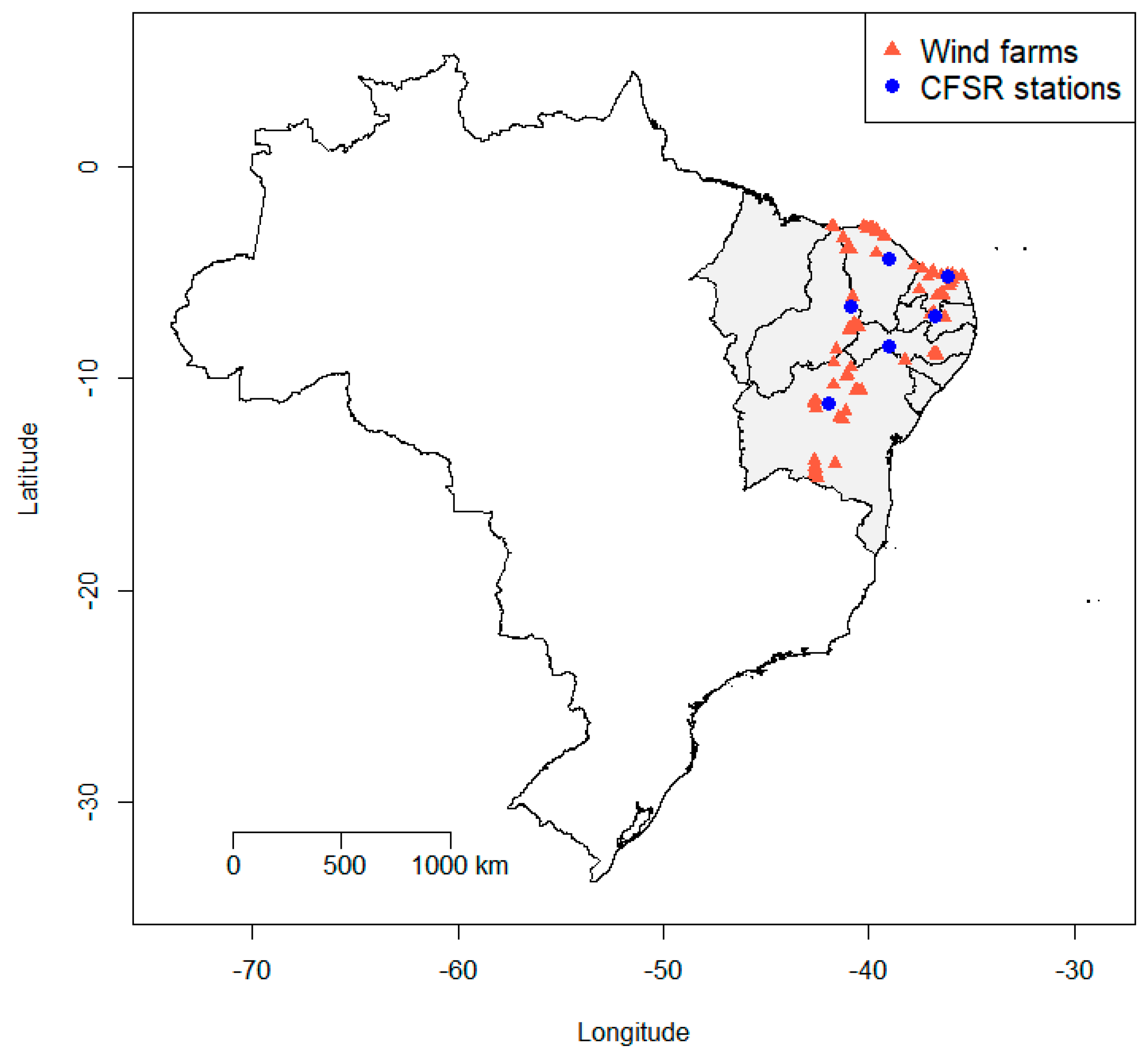
The Northeast region is composed by the states of Alagoas, Bahia, Ceará, Maranhão, Paraíba, Piauí, Pernambuco, Rio Grande do Norte and Sergipe, and has the longest coastline of the country’s regions (3000 km). According to the National Electric Energy Agency (Agência Nacional de Energia Elétrica—ANEEL), in July 2017 there were 209 wind farms in operation, accounting for 3.6 GW of installed capacity, 172 under construction or due to start construction in the near future, totaling an addition of approximately 4 GW in this region in the following years. Of these 172 wind farms under construction, only 74 will be in operation within the study horizon, totaling 283 undertakings considered for all future calculations.

Figure 3 shows a map of the Northeast region and the location of wind farms. Note there is a concentration along the coast, but a considerable number are also located in the interior.

3.1. Obtaining the Historical Measurements Per Wind Farm

As mentioned above, the wind speed series were obtained from the CFSR system and the measured point to be used is the closest one to each wind farm. Following this, only 6 measurement points were needed and the maximum distance found was approximately 12 km.

Table 1. Latitude and longitude of CFSR measurement stations.

Station	Latitude	Longitude
NASA 1362	−4.40	−39.07
NASA 1628	−5.21	−36.20
NASA 2046	−6.64	−40.91
NASA 2192	−7.05	−36.82
NASA 2622	−8.48	−39.07
NASA 3427	−11.14	−41.93

shows the latitude and longitude of each measurement station of the CFSR system.

A survey of the turbine models installed at each wind farm revealed that only 7 turbine manufacturers serve this region with 12 models.

Table 2. Manufacturers, models and technical information.

Manufacturer	Model	Hub Height (m)	Cut-in Wind Speed (m/s)	Rated Wind Speed (m/s)	Cut-Off Wind Speed (m/s)	Rated Power (kW)
Acciona	AW-3000/116	120	3	10.6	20	3000
Alstom	ECO-122/2700	139	3	10	25	2700
Alstom	ECO-86/1670	80	3	10	25	1670
Gamesa	G106/2500	93	2	12	24	2500
Gamesa	G97/2000	120	3	14	25	2000
GE	1.6-100	100	3.5	11	25	1600
GE	1.85-82.5	80	3	13	25	1850
GE	1.7-103	96	3	10	23	1700
GE	1.68-100	100	3.5	11	25	1680
Siemens	SWT-2.3-101	100	3	12	20	2300
Weg	AWG 110/2.1	120	2.5	11	20	2100
Wobben	E92/2350	138	2	13	25	2350

presents the manufactures, models and technical parameters.

In this same step, the height correction factor is calculated, considering that the measurements are made 10 m above ground. The maximum wind turbine height found was 139 m and the minimum was 80 m, so the height correction factor varies from 1.90 to 2.14.

Therefore, by combining the Weibull distribution and the wind speed time series obtained from the CFSR system it was possible to obtain the expected wind power time series for each of the 283 wind farms. The year 2016 was used as calibration year, so for each wind farm, expected wind power is multiplied by a monthly calibration factor obtained through the relation between calculated and observed monthly generation. This calibration factor is calculated using monthly data since the observed wind power generation is available on a monthly basis. For the 74 farms that will be in operation, the monthly average of the calibration factor of the others plants was applied.

3.2. Wind Power Simulation Model Results

The first task in this stage is the transformation of the wind power obtained in the previous step into a finite number of states. To do this, we applied the K-means clustering technique where at least 98% of the data variability has to be represented, resulting in a variation from 13 to 24 in the number of clusters when applying the methodology to the wind power data, with great concentration around 15 clusters. The number of clusters varies accordingly to the original wind power data distribution, without any external interference.

The next step involves calculating the Markov chain transition matrix, constructed by the frequency at which one state transits to another, or to itself. As an example, in

Table 3. Transition matrix example.

State a (MW)	State b (MW)
	0	0.32	1.20	2.18	3.32	4.47	5.71	7.03	8.57	10.20	11.77	13.55	15.53	17.60
0	0.50	0.50	0	0	0	0	0	0	0	0	0	0	0	0
0.32	0.01	0.84	0.13	0.02	0	0	0	0	0	0	0	0	0	0
1.20	0	0.14	0.58	0.25	0.03	0	0	0	0	0	0	0	0	0
2.18	0	0.04	0.21	0.41	0.28	0.04	0.03	0	0	0	0	0	0	0
3.32	0	0	0.05	0.20	0.34	0.23	0.06	0.08	0.02	0.02	0	0	0	0
4.47	0	0	0.02	0.07	0.22	0.31	0.24	0.10	0.03	0.00	0	0	0	0
5.71	0	0	0	0.04	0.07	0.21	0.29	0.21	0.09	0.07	0.02	0	0	0
7.03	0	0	0	0.03	0.03	0.10	0.24	0.32	0.15	0.06	0.05	0.02	0	0
8.57	0	0	0	0.00	0.02	0.06	0.04	0.21	0.31	0.17	0.08	0.08	0.04	0
10.20	0	0	0	0.00	0	0	0.04	0.09	0.26	0.24	0.26	0.07	0	0.04
11.77	0	0	0	0.02	0	0.02	0.02	0.05	0.11	0.30	0.23	0.11	0.11	0.02
13.55	0	0	0	0	0	0	0	0	0.08	0.04	0.31	0.31	0.15	0.12
15.53	0	0	0	0.04	0	0	0	0	0	0.11	0.19	0.11	0.30	0.26
17.60	0	0	0	0	0	0	0	0.03	0	0	0.02	0.03	0.14	0.78

the wind farm Abil transition matrix of March is presented. First, notice that the time series of this wind farm was divided into 14 finite numbers. Note also that the transitions happen in a gradual way, that is, if at a moment the generation is low, the chance that in the next moment this value is high is almost zero or zero in many cases, while the opposite is also true.

To build the cumulative transition matrix it is necessary to add for each state the probability of the previous states with their own probability. See

Table 4. Cumulative transition matrix example.

State a (MW)	State b (MW)
	0	0.32	1.20	2.18	3.32	4.47	5.71	7.03	8.57	10.20	11.77	13.55	15.53	17.60
0	0.50	1	1	1	1	1	1	1	1	1	1	1	1	1
0.32	0.01	0.85	0.98	1	1	1	1	1	1	1	1	1	1	1
1.20	0	0.14	0.72	0.97	1	1	1	1	1	1	1	1	1	1
2.18	0	0.04	0.25	0.66	0.93	0.97	1	1	1	1	1	1	1	1
3.32	0	0	0.05	0.25	0.59	0.83	0.89	0.97	0.98	1	1	1	1	1
4.47	0	0	0.02	0.09	0.31	0.62	0.86	0.97	1	1	1	1	1	1
5.71	0	0	0	0.04	0.11	0.32	0.61	0.82	0.91	0.98	1	1	1	1
7.03	0	0	0	0.03	0.06	0.16	0.40	0.73	0.87	0.94	0.98	1	1	1
8.57	0	0	0	0	0.02	0.08	0.12	0.33	0.63	0.81	0.88	0.96	1	1
10.20	0	0	0	0	0	0	0.04	0.13	0.39	0.63	0.89	0.96	0.96	1
11.77	0	0	0	0.02	0.02	0.05	0.07	0.11	0.23	0.52	0.75	0.86	0.98	1
13.55	0	0	0	0	0	0	0	0	0.08	0.12	0.42	0.73	0.88	1
15.53	0	0	0	0.04	0.04	0.04	0.04	0.04	0.04	0.15	0.33	0.44	0.74	1
17.60	0	0	0	0	0	0	0	0.03	0.03	0.03	0.05	0.08	0.22	1

for the cumulative transition matrix for the Abil wind farm in March.

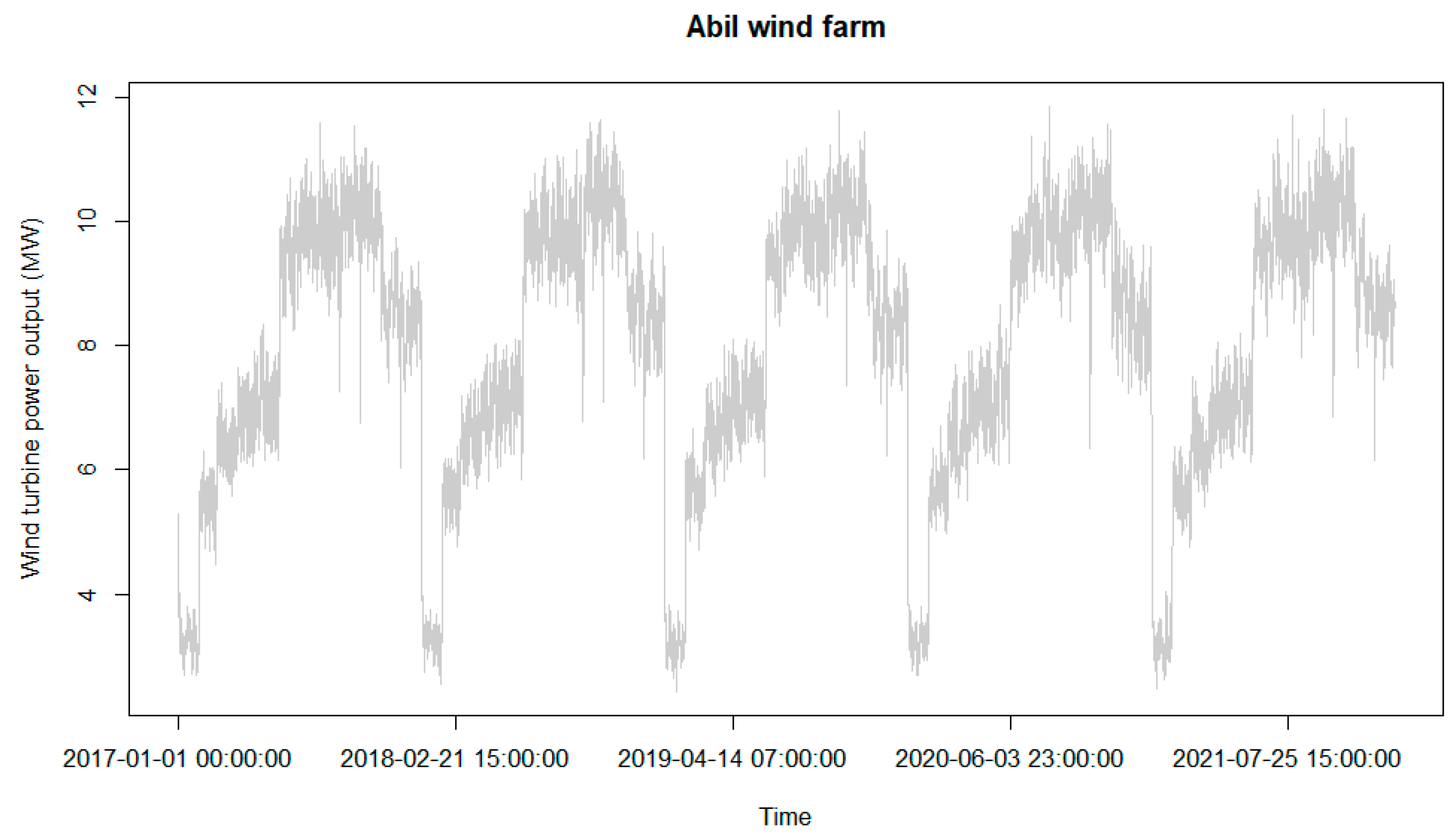
To simulate the hourly wind power values, it is first necessary to randomly select the initial state, for instance, state 3 (1.20 MW in the example) and then to choose a value from the uniform [0, 1] distribution. Assume it is 0.92. This means that the first simulated value is 1.20 MW and the second is 2.18 MW, since 0.92 is more than 0.72 (state 3) and less than 0.97 (state 4). This procedure continues until the entire horizon has been simulated for each wind farm. For convergence reasons, this entire process was repeated 200 times, thus generating the same number of possible scenarios. This value was chosen after performing sensitivity analysis of this database for different numbers of scenarios. Figure 4 depicts the average scenarios for the Abil farm.

In Figure 4 it is not possible to see the year-to-year variation of the wind series, but since the dispatch is optimized using the farms in aggregate form (submarket) rather than individually, the year-to-year variations are not significant, because in this case, the generation variation of a farm may be compensated for the others. Still, the year-to-year wind generation of the submarket is represented by considering the entry of new farms into operation in the future.

3.3. Checking of the Wind Power Simulation Model Results

In order to check the goodness of the simulated series, statistical factors were considered, such as the probability distribution function (PDF), autocorrelation functions (ACF), monthly characteristics and Wilcoxon signed-rank test.

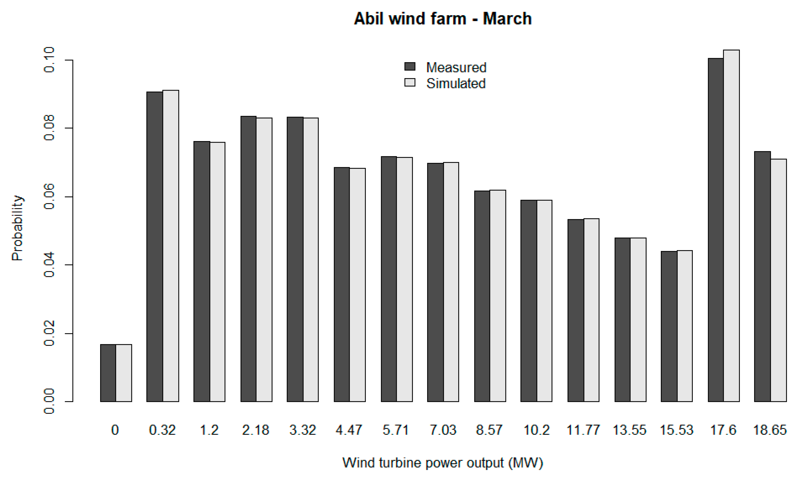
The PDF shows the values of the distribution behavior of a given database. In this work it is used to compare the proportion of values generated through the simulation and the real series. Note in Figure 5 that the number of values belonging to a state in the simulated series is approximately equal to that of the real series, indicating that the synthetic scenario generation method used satisfactorily reproduces such behavior.

Given that the wind time series behave differently between the seasons of a year, it is important to check whether the means and variations between the months are replicated for the simulated series compared to the measured series.

Table 5. Monthly results.

Month	Mean (MW)		Standard Deviation (MW)
	Measured Data	Simulated Data	Measured Data	Simulated Data
Jan	3.2204	3.2727	3.5331	3.5668
Feb	5.6109	5.5751	4.2978	4.3025
Mar	6.3998	6.4795	5.3218	5.3187
Apr	7.0073	6.9852	5.6116	5.6165
May	7.1462	7.1800	5.8127	5.8084
Jun	9.0496	9.3804	6.3166	6.3166
Jul	9.9104	9.9181	6.0918	6.1196
Aug	9.6687	9.7155	6.2547	6.2793
Sep	10.5886	10.2190	6.5827	6.6192
Oct	10.1114	10.2143	6.3178	6.3066
Nov	9.1185	8.7986	6.7229	6.6391
Dec	8.2729	8.3653	6.3252	6.3179

shows the mean and standard deviation values obtained from the measured data and the simulated data. Notice that the values of both, the simulated and observed series are very close, with the percentage errors varying from 0.08% to 3.64% for the mean and 0.00% to 1.26% for the standard deviation. This indicates that the scenario generation method replicates the inherent variation of the wind series.

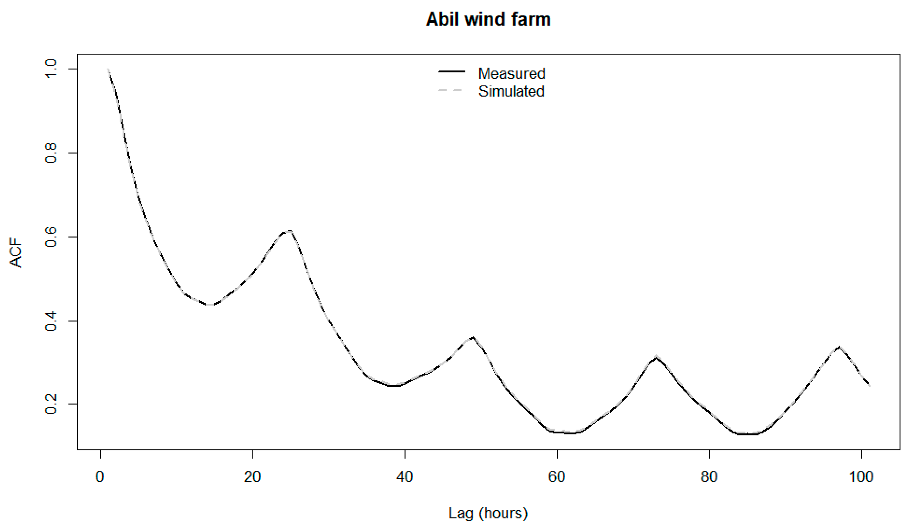
In the previous analysis we checked whether the wind series seasonal behavior was replicated in the simulated series. In the present analysis, we check if the intra-hour behavior is reproduced using the autocorrelation function, which presents the correlation between the time intervals. Figure 6 shows that the peaks are exactly in the multiple of 24 lags, and since we are dealing with an hourly time series, it is possible to conclude that the present method also reproduces the hourly behavior.

The last feature to be tested is whether the simulated series fits the same distribution of the real data. In order to do that, the Wilcoxon signed-rank test was used (since the data were not normally distributed). The test’s null hypothesis is that both distributions are equivalent, and since the p-value obtained is 0.2929, it is possible to conclude that the probability distribution of the simulated data is the same as the measured data.

3.4. Creating Hourly Load Values

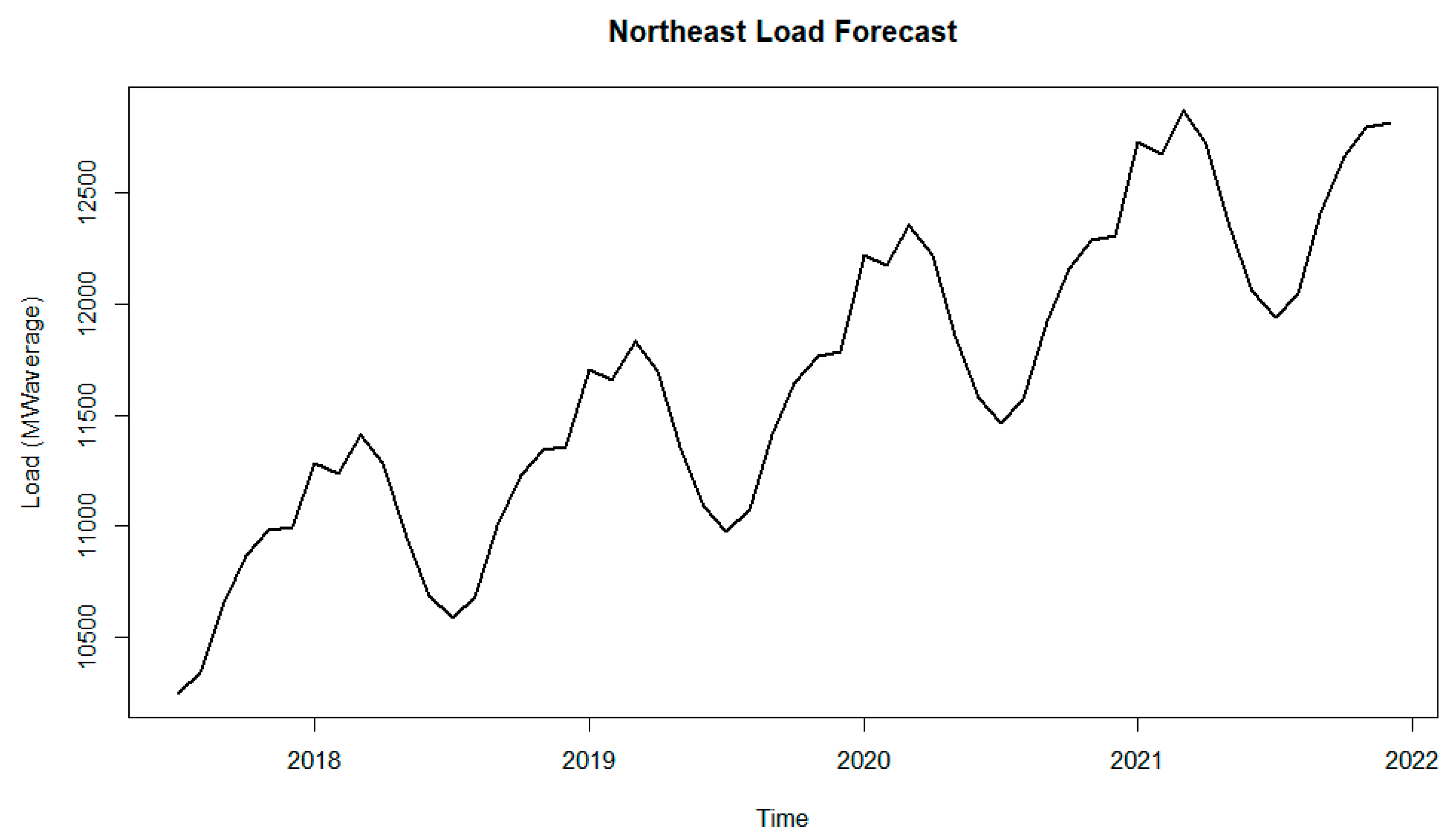
As stated in Section 2.3, it is not possible to obtain hourly load forecasts directly from official organizations. Therefore, a methodology was developed to obtain such data from the load expectations made available for 60 months on monthly basis (Figure 7).

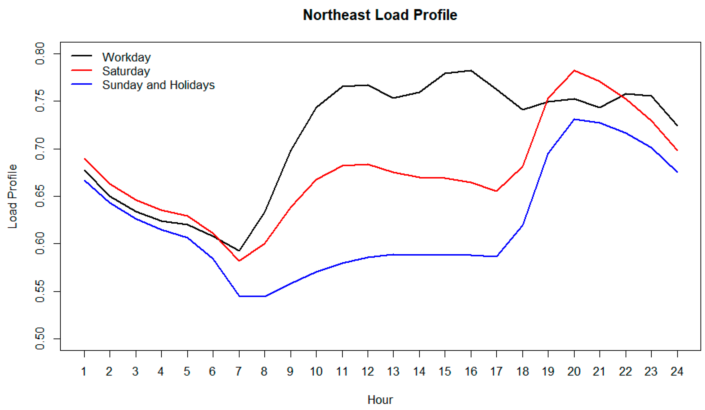
The first step involves obtaining the load profiles by type of day (workday, Saturday and Sunday/holidays) and month from a historical time series. Figure 8 presents the average monthly profiles for the Northeast submarket using data from January 2008 to December 2017. Note that during the early morning hours (1 a.m. to 5 a.m.) there is no significant difference in load between profiles, with the lowest values being on Sundays and holidays. However, during business hours (8 a.m. to 5 p.m.) there is a big difference between the profiles, where on weekdays the average load is much higher than on other days, as expected. In the evening (7 p.m. to 9 p.m.), this behavior is reversed, with higher load on Sundays and holidays.

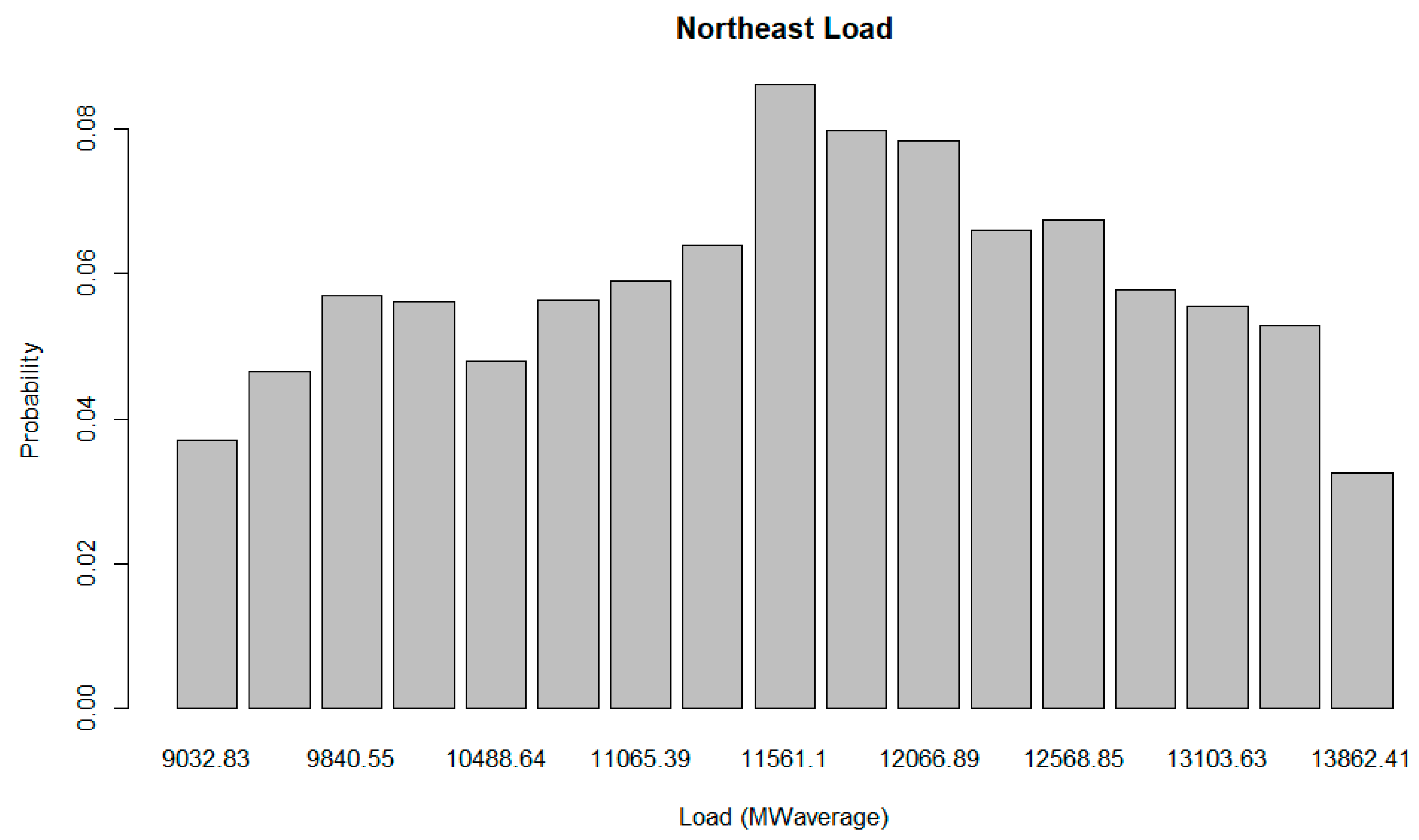
By combining Figure 7 and Figure 8, it is possible to transform the monthly forecast into hourly forecast, not displayed graphically for complexity reasons. The next step involves discretization of time series into finite values, just as was done for the wind power time series. The K-means process produced 17 clusters (Figure 9), accounting for 99.5% of the total data variation.

3.5. Net Demand and Optimization of Dispatch Results

Now that all the information needed to calculate the net demand is available, it is possible to obtain the final results and compare then with those expected by the government.

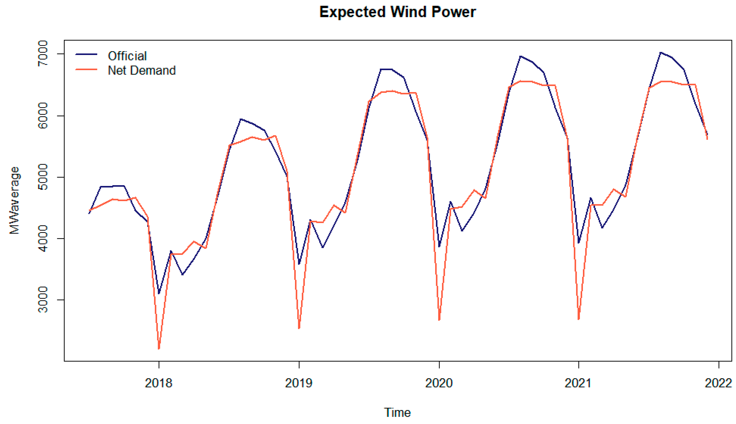
The first and most important result is the wind generation forecast for the next 5 years (or 60 months). In Figure 10, the forecast through the net demand approach and from the official sources are presented, where it is possible to observe that, on average, wind power generation predicted by the government is higher than the simulated value, especially regarding peaks and valleys. Apart from this, both have the same trend and behavior.

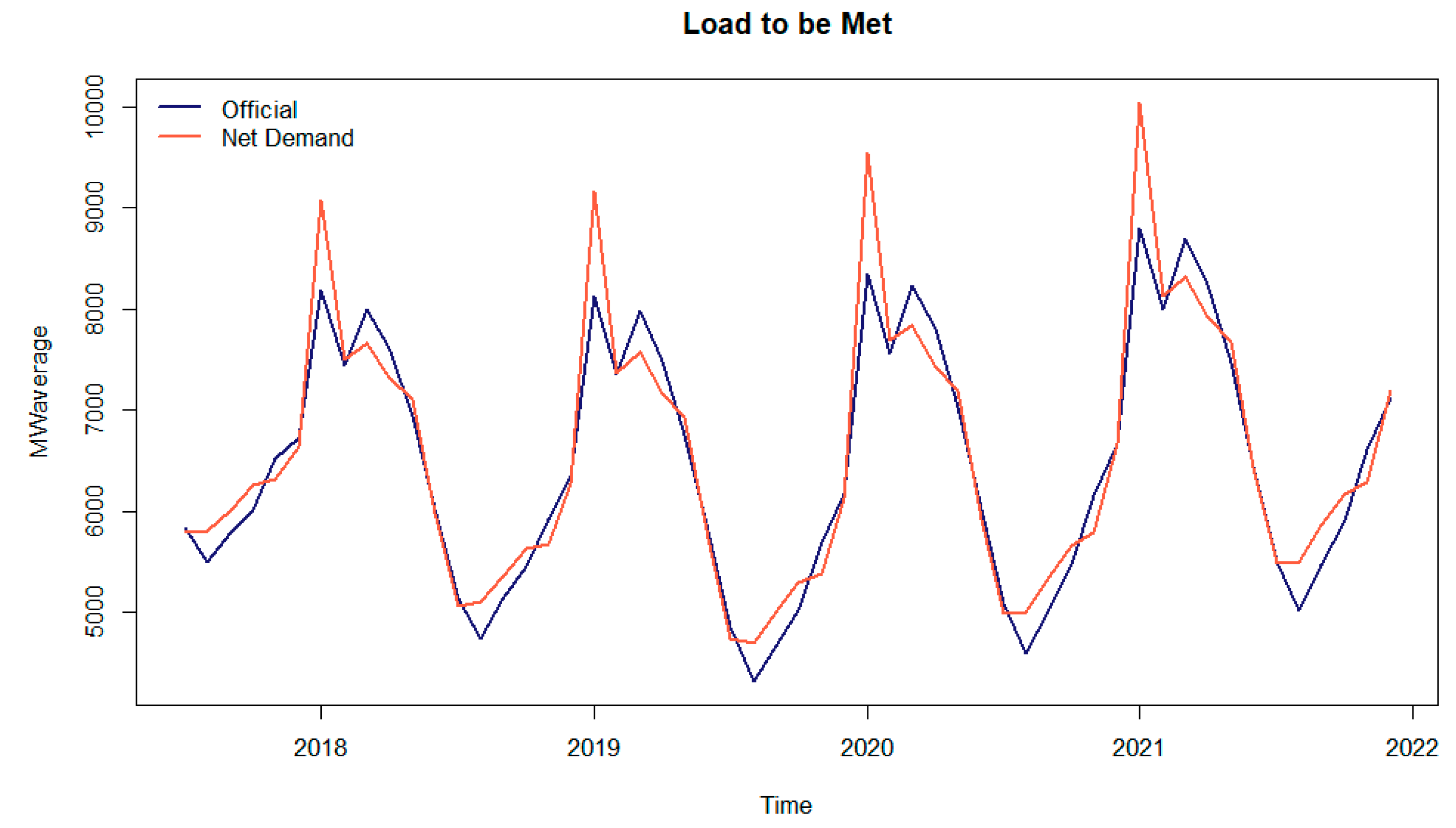
As a consequence of a smaller expected wind power availability in the future compared to the official expectations, the load to be met (Figure 11) will present higher values when considering the methodology proposed here.

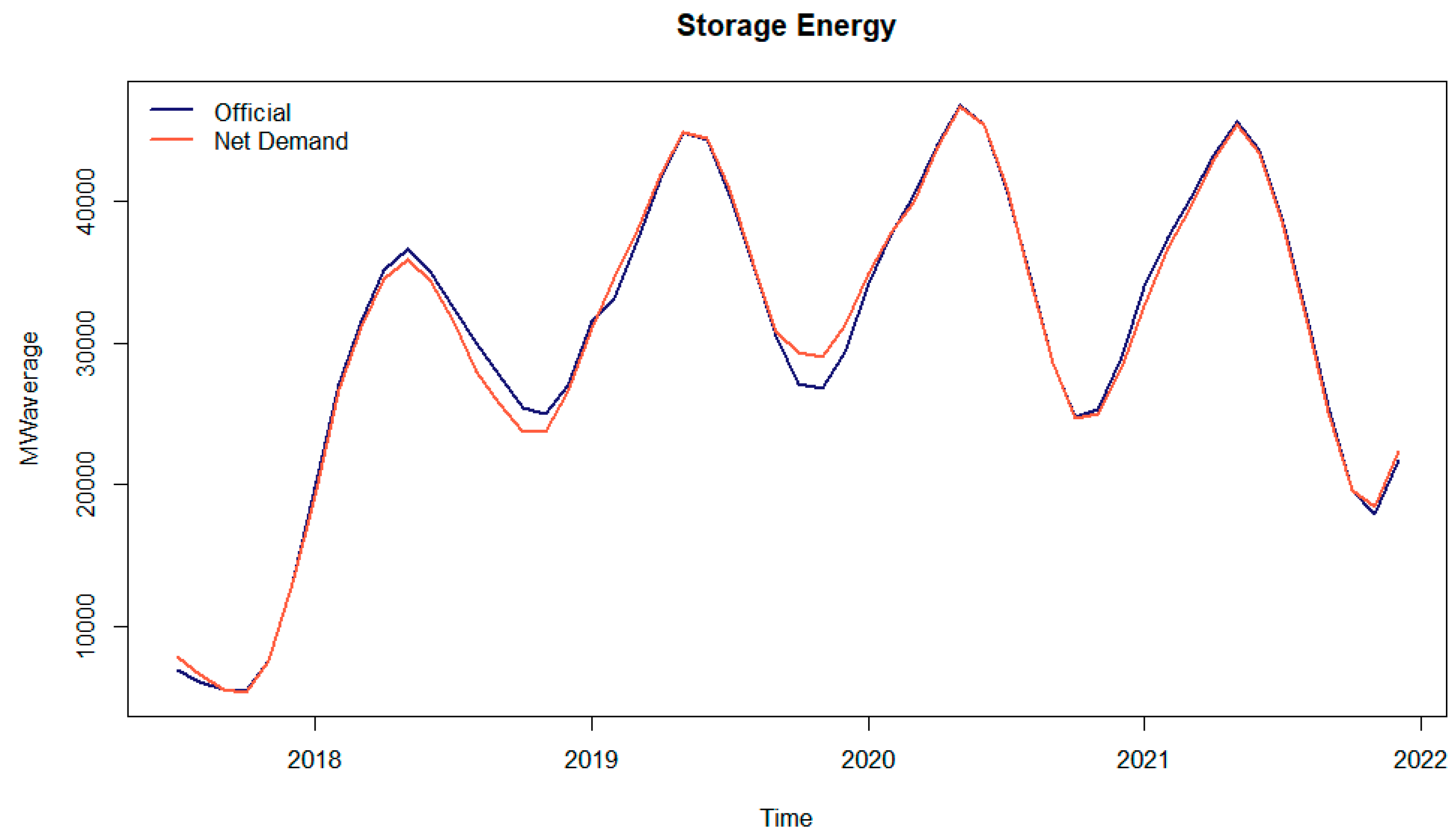
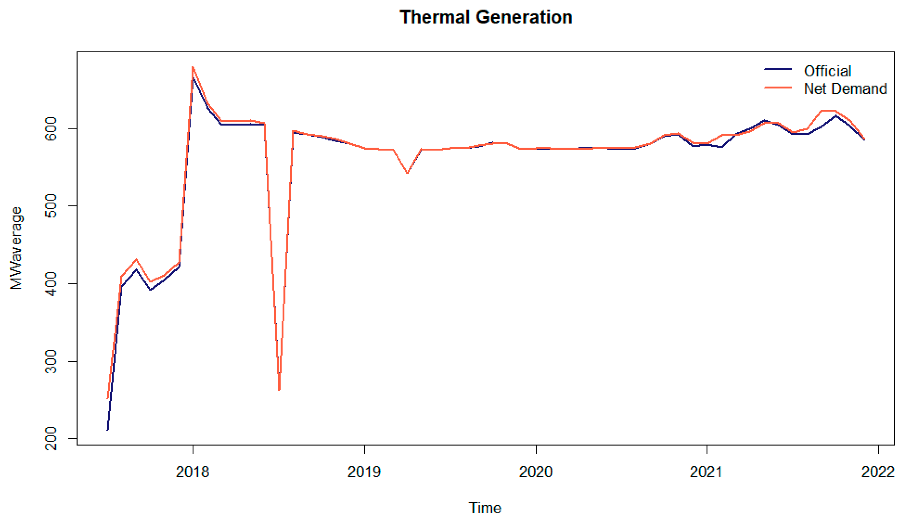
Considering the data from the load to be met (Figure 11), it is possible to evaluate, using the optimization dispatch model, the system’s behavior according to the power demand forecasts and simulated wind power generation. Figure 12 presents the energy storage and Figure 13 gives the thermal generation according to official sources and the net demand approach. From Figure 12 it is possible to notice that the energy stored considering the official forecasts is almost the same as in the net demand approach, but in the dry season the proposed methodology is more conservative.

For the thermal generation, since with the net demand approach a more conservative generation of wind energy is expected, the complementation with thermal generation will be larger, as shown in Figure 13. Note that there was a drop in thermal dispatch in 2018, July 2018. In this month, it is possible to see that the load was low (the lowest level in 2018), and in addition, the income inflow contributed in a manner that it was not necessary to dispatch thermal power plants, since the hydro generation could supply most part of demand. It is important to emphasize that this is a part of the optimization results, restricted to the Northeast Brazil’s region.

4. Conclusions

This article proposes an approach to incorporate wind power generation in the current Brazilian hydro-thermal dispatch. The methodology is summarized in three main stages, comprising fourteen distinct steps, where the first stage deals with historical measurements, the second stage with the wind power simulation via MCMC and the final stage with the net demand calculation. The historical measurement stage involves obtaining wind speed data from a reanalysis database and transformation to wind power by the Weibull probability distribution. A wind power scenario, based on the MCMC model, is created for the entire time considering the starting date of operation of each wind farm. From statistical factors, the simulated time series characteristics are tested and validated in comparison with the observed series that replicate the monthly and hourly behavior and also the temporal correlation together with the probability distribution. In the net demand stage, a standard load profile by type of day is computed and applied to the monthly load forecasting, followed by the discretization of both the generation and the load series into finite states. In this stage, the Markov chain transition matrices and steady-state probabilities are also estimated. The combination of generation and load states into a single net demand value for each month of the planning period is performed by discrete convolution and expected value calculation.

The results obtained confirm that the expected wind power forecast using the proposed methodology is more conservative than the official expectations. That is, in periods of higher wind power generation in the Northeast, the net demand approach expects less generation than the government, with the same for periods with smaller generation. Thus, the load to be met will be greater according to the methodology proposed here. These values indicate a lower expectation of water storage in the future, translated into energy storage, and also higher generation from thermal plants. The main consequences of such differences between what is expected by the government and the forecast calculated here are the depletion of hydroelectric reservoirs and also the “non-optimization” of dispatch. Therefore, we can conclude that the consideration of probabilistic scenarios of wind energy generation as proposed in the net demand approach can mitigate errors in decision making by the Brazilian National Electric System Operator.

Finally, our objective was satisfactorily achieved, since the suggested methodology was able to: (i) reproduce the variable behavior of the wind series; and (ii) insert the wind generation in the current optimization dispatch model, conserving its structural mathematical formulation.

For future research, we suggest using other databases to provide wind speed series in addition to obtain a history of more than one year in order to capture yearly variability. We also suggest the application of other techniques to forecast wind power generation and consideration of different approaches for insertion of such generation in a mainly water and thermal dispatch. The application of methods that specifically consider the night/day effects of wind time series is another suggestion. We also recommend the construction of confidence intervals to increase the reliability of the applied simulation method, as was done in Cyrino Oliveira et al. [45] using bootstrap, or as it was done in Yang et al. [46] by applying Markov chain methods. Finally, it is possible to apply the proposed approach to other renewable sources, such as photovoltaic.