Abstract
The shift from fossil fuel to more renewable electricity generation will require the broader implementation of Demand Side Response (DSR) into the grid. Utility processes in industry are suited for this, having a large thermal time constant or buffer, and large electricity consumption. A widespread utility system in industry is an induced draft evaporative cooling tower. Considering the safety aspect, such a process needs to maintain cooling water temperature within predefined safe boundaries. Therefore, in this paper, two modelling methods for the prediction of the basin temperature of an induced draft evaporative cooling tower are proposed. Both a white box and a black box methodology are presented, based on the physical principles of fluid dynamics and adaptive neuro-fuzzy interference system (ANFIS) modelling, respectively. By analysing the accuracy of both models with a focus to cooling tower fan state changes, i.e., DSR purposes, it is shown that the white box model performs best. Fostering the idea of using such a system for DSR purposes, the concept of design for flexibility is also touched upon, discussing the thermal mass. Pre-cooling, where the temperature of the cooling water basin is lowered before a fan switch off period, was simulated with the white box model. It was shown that beneficial pre-cooling (to lower the temperature peak) is limited in time.
1. Introduction
The European Union’s long-term strategy calls for a decarbonised electricity generation and sets a target of 80% renewable electricity generation by 2050 [1]. Today, the large majority of the electricity generation in Europe is based on fossil fuels. By means of these controllable and often flexible fossil fuel power plants, the electricity generation has always followed the electricity consumption, serving the demand–supply balance. In the light of Renewable Energy Sources (RES) integration into the electrical grid, the assumption of electricity generation following the demand is to be questioned. As RESs are by nature not continuously available and often unpredictable, the concept of Demand Side Response (DSR) gains more interest [2]. Being able to shift electricity consumption in time can contribute to the amount of RES which can be integrated into the electrical grid [3], fostering the long-term goal of the European Union.
When looking for DSR opportunities, often the heads are turned towards the industry. Electrical intensive processes could be identified, adapted and controlled so to serve the purpose of keeping the electricity demand supply balance. By assessing the possibilities in the chemical process industry, the utilities processes are identified as having DSR potential for the reason of having a buffer or large thermal time constant [4]. One of these utilities processes, evacuation of process waste heat by use of an induced draft evaporative cooling system, is the focus of this work.
An induced draft evaporative cooling tower could be used as a DSR controlled system, linking a thermal profile with a rather large time constant to a faster fan control strategy. When operating a cooling system with non Variable Speed Drive (VSD) controlled fans, only a discrete number of fan operating states are possible. While the water basin temperature setpoint (Ts) is pursued, hysteresis (with a lower Th, min and upper Th, max limit) prevents the continuous control of the fans (switching on or off, to low or high speed states). A minimum (Tmin) and maximum temperature (Tmax) is set to ensure the process efficiency and safety. It is this hysteresis zone combined with the other control zones which could be beneficially used to develop a control strategy for the fans, creating the opportunity of economic optimisation. This is shown in Figure 1.
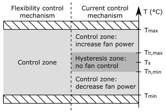
Figure 1.
Graphical representation of control zones for non-VSD controlled cooling systems.
Cooling towers are designed based on static calculations taking into account the maximum heat load to be dissipated. Often, no dynamic thermal model is available, resulting in the inability to assess the impact of fan control without practical tests. To be able to verify a fan control strategy, the temperature of the cooling water needs to be simulated. Therefore, this paper proposes two modelling methods for predicting the water basin temperature. The proposed white box and black box models find an equilibrium between model complexity and model response accuracy, fostering the implementation in a real-life industrial setting. To the best of our knowledge, this approach for a DSR application of an industrial-sized induced draft evaporative cooling system has not been presented in the current literature.
The remainder of this paper is structured as follows. In Section 2, a brief explanation of an induced draft evaporative cooling system is given, including the parameters as presented at a chemical industry site of INEOS in Belgium. In Section 3.1 and Section 3.2, the black box and white box models are developed and validated for fan state changes in the dataset, respectively. In Section 4.1 the concept of design for flexibility is touched upon, considering the thermal mass of the system. The concept of pre-cooling is explained in Section 4.2.
2. Evaporative Cooling System
The cooling system under investigation in this paper is based on evaporation. The physical state change from a fluid, i.e., water, to a gas, i.e., water vapour, requires latent heat. This heat is extracted from the water, resulting in a temperature decrease. Together with the heat evacuation, also mass leaves the system under the form of water vapour. In an industrial setting, this physical phenomenon is exploited by spraying warm water in a cooling tower, where a counter airflow is induced by fans to maximise the air–water interaction. As a result, the water falling down in the basin underneath has dropped in temperature and can be recirculated through the process. For a more detailed description of an induced draft evaporative cooling system, we refer to [5]. The models created in this work are based on and verified by the data from an industrial cooling system as available at a chemical industrial site of INEOS in Belgium. The system details and parameters are given in Section 2.1.
2.1. INEOS Cooling System
Figure 2 is a simplified graphical representation of the existing system at a chemical industrial site of INEOS in Belgium. Cooling water is circulated by use of induction motor driven pumps P1 and P2. The water flows through the heat exchangers (HEX) evacuating the heat from the production process. There are two cells in the cooling tower, each with a fan (F1 and F2) driven by a Dahlander motor. One single water basin is available for both cells and has a capacity of 900 m3.
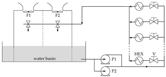
Figure 2.
Simplified graphical representation of an induced draft evaporative cooling system.
2.1.1. Design
The cooling system is designed for a water flow rate of 950 kg/s with a process water temperature of 36 C and a range of 9 C while the wet bulb temperature is 22 C [6]. The heat to be evacuated, i.e., process heat , at these design parameters is thus 35.79 MW according to Equation (1) with a basin water temperature of 27 C and the correct specific heat capacity of water .
As explained in Section 1, the cooling system is indeed designed based on static calculations. The given process heat to be evacuated is therefore only valid under the aforementioned conditions.
Both cooling tower cells are identical; they feature a 12-blade fan with a diameter of 6.1 m and a cell size of 11 m by 11 m [6]. One cooling water pump, P1, is active in normal operation, delivering a flow close to the designed water flow rate of 950 kg/s. P2 is used as a backup pump with a nominal flow of 639 kg/s. Multiple heat exchangers are installed throughout the production facility, which can be controlled by valves (V) at the upstream side. In this work, the focus lies on the tower side of the cooling network, therefore a single heat source for the process heat is assumed. This is further explained in Section 3.2.1.
The cooling tower fan Dahlander motors have a rated power of 110 kW when operating at high speed and 25 kW when operating at low speed; the rated speeds are 1500 rpm and 750 rpm, respectively. The motor efficiencies are given in the datasheet [6] for three motor load points per speed, as shown in Figure 3.
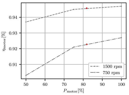
Figure 3.
Efficiencies of the Dahlander motors driving the fans. The working point is indicated with a red dot.
A measurement was installed on one of the motors to obtain the actual power consumption in both high speed and low speed working modes. For the Dahlander motor of F1 a value of 89.73 kW and 20.5 kW was obtained for high speed and low speed modes, respectively. As both cooling tower cells are identical, it is assumed that these figures are also valid for F2. The pitch angle of the blades of both fans is fixed, resulting in a stable power consumption for each of the operating modes. By interpolating between the two given motor load points of 75% and 100% nominal power, values of 0.946 and 0.924 are obtained for the high speed and low speed modes, respectively. In Figure 3, the efficiencies are shown in red.
The Dahlander motor is connected to the fan by means of a gearbox with a ratio of 11.6 to 1, resulting in fan speeds of 129 rpm and 64 rpm in high speed and low speed modes, respectively. No efficiency is given for the gearbox.
2.1.2. Operation
The cooling system is controlled by skilled process operators, who will switch the fans in function of the water basin temperature. In practice, as the fan control is not automated, the fans are switched infrequently. A summer and winter regime is applied, where the fans are, respectively, both switched on to high setting or one fan is switched on to high setting and the other is switched off. Only in the case of process upsets or extreme weather conditions, i.e., when temperature is expected to exceed the safety boundaries (Tmax, Tmin), the fans are switched on–off. A very stable water flow rate is observed as no changes are made to the valves or pumps during operation.
2.1.3. Data Availability and Pre-Processing
A SCADA system is used on the INEOS industrial site to collect and organise all the data from various systems. Available measurements on the cooling system are given in Table 1. The data have an interval of 15 min.

Table 1.
Available data on the INEOS industrial site.
Data preprocessing is done on the dataset. It is expected that the data are noisy as they are imported directly from the INEOS site SCADA system. Corrupt records, due to faulty sensors, and outliers are removed. In total, 32,617 rows of data are retained.
3. Cooling Tower Modelling
The goal of the developed cooling tower model is to define the electrical flexibility of the system at every moment in time, using the water basin temperature as limiting factor. Electrical flexibility is defined as a change in electricity consumption due to an external signal. Controlling the fans changes both the electricity consumption of the cooling system, i.e., the sought electrical flexibility, and the water basin temperature. As discussed in Section 1, the temperature of the water basin needs to be maintained within certain boundaries for safe process operations. By simulating and predicting the response of the water basin temperature to a fan state change, an estimate for the electrical flexibility can be made. Therefore, in this work, a model of an induced draft evaporative cooling tower is developed focusing on the accuracy for fan state changes. Two modelling approaches, black box and white box, are considered.
3.1. Black Box
A possible modelling approach is the black box method. Black box modelling is useful when the first objective is to fit the data and identify the dynamics of the system regardless of particular differential equations and mathematical structures of the model. In this way, the response of the model to input changes can be evaluated. Black box models can be constructed making use of system identification techniques, e.g., Artificial Neural Networks (ANN) or Adaptive Neuro-Fuzzy Interference System (ANFIS). The method is also referred to as a soft computing technique due to the lower engineering effort compared to white box modelling [7].
In [8], Pan et al. proposed a multi-model method for assessing the performance of a cooling tower based on Local Model Networks (LMN). To structure the data into groups where linear models can be applied, the Fuzzy C-Means (FCM) clustering technique is used based on Lloyd’s algorithm [9]. An algorithm is used to integrate the FCM into the LMN, so to automatically optimise the amount of created clusters [9]. Abdalla et al. also proposed a method to assess the operating performance of a cooling system [10]. The studied cooling system is made up with absorption, water-cooled and air-cooled chillers of which the primary sides are connected to a cooling tower. The followed methodology by Abdalla et al. is to optimise the output of the ANFIS-based FCM or Fuzzy Subtractive Clustering (FSC) with Accelerated Particle Swarm Optimisation (APSO).
3.1.1. Prerequisites and Limitations
The development of a black box model requires the availability of data to train the model, implying that the system needs to be fully operational for some time and that data are collected. The developed model is only valid within the range of the inputs and outputs of the used training dataset. As an induced draft evaporative cooling tower is subject to weather influences and seasonality, the model should be developed using a dataset covering the complete spectrum, i.e., including very low and very high temperatures. Indeed, to develop the black box model in this work, a dataset spanning a complete year is used, with ambient temperature extremes of −5.84 and 34.6 .
The developed black box model is limited in use to the specific system at the INEOS industrial site, on which it was developed. Evaluating the electrical flexibility potential of other forced draft evaporative cooling systems requires a complete new model to be developed. Adaptations to the existing system at the INEOS industrial site, e.g. the addition of a cooling tower cell, would also require a new model to be developed. In the latter case, the system would also need to run for a certain amount of time with the new configuration, to collect the necessary data for the black box modelling approach.
3.1.2. Model Development
To implement the black box modelling approach, it was decided to create an Adaptive Neuro-Fuzzy Interference System (ANFIS) model. While the ANFIS technique was already developed in 1993 by Jang et al. [11], only quite recently the technique was applied on cooling systems [7,8,10]. As the goal of the developed black box model is to simulate the water basin temperature in a practical way and in an industrial setting, the input parameters are limited to the readily available information on the INEOS industrial site. This approach yields a total of five input parameters, being , , , , and , and one output parameter being . Details on these inputs and output can be found in Table 1. The electric current of pump P2, , could also be included, but is here neglected as the pump was not active during the considered time period. The water flow rate is directly correlated to and is therefore not maintained as an input parameter.
The ANFIS technique is based on the training of an Artificial Neural Network (ANN) with an interference system based on fuzzy rules. The dataset is split into a non-overlapping training and testing dataset. The dataset used in this paper is from the INEOS industrial site and contains 32,617 rows, as explained in Section 2.1.3. Further data pre-processing is done using a min-max normalisation on all five inputs, as there are large differences in value ranges. This prevents the inputs with larger values from influencing the result more. As the last step, the dataset is randomly divided into a training and testing dataset with commonly used 70% and 30% sizes, respectively. The random division ensures that the seasonality of the data is not reflected in either only the training or testing dataset.
The Fuzzy C-Means (FCM) method is used to generate a Sugeno type initial Fuzzy Interference System (iFIS) from the given training data. The used criteria of 0.5 for the radii and inclusion of the outer values for both the inputs and output yields an iFIS with five clusters, five rules and five Membership Functions (MFs). The iFIS is now used to train the model so to tune the parameters. A hybrid learning algorithm combining the back-propagation and least-squares gradient descent methods is used. Figure 4 gives a schematic representation of the used methodology. The testing dataset is used to verify that the number of training cycles, i.e., epochs, is chosen correctly to prevent the possible over-training of the network, which would result in overfitting. In Figure 5, it can be seen that the optimal number of epochs for the generated cooling tower FIS is 232, resulting in a Root Mean Square Error (RMSE) of the testing data of 0.879.
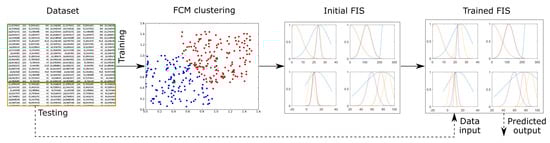
Figure 4.
Structure of used ANFIS modelling methodology.
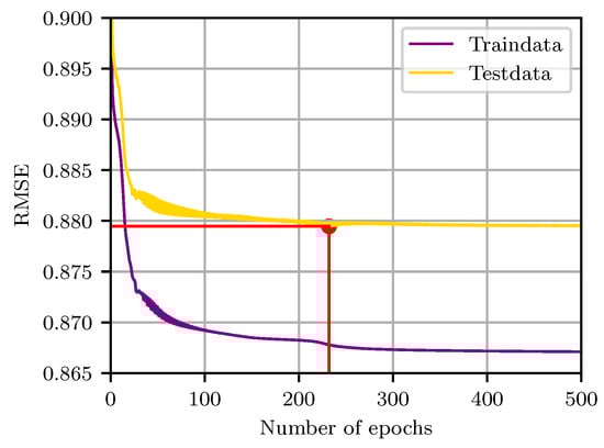
Figure 5.
The optimal number of training epochs is 232, resulting in an RMSE of the testing data of 0.879.
3.1.3. Analysis
The RMSE of 0.879 found in Section 3.1.2 is based on the testing data, i.e., a random 30% of the total dataset, containing data points for all system states and possible transients between those states. As the purpose of the model is to define the water basin temperature change for potential activations of the electrical flexibility, i.e., changing the state of the fans, detail is given to these temperature responses. A total of 13 fan state changes available in the dataset are envisaged. Figure 6 shows one of the water basin temperature responses, during a period of 6 h starting from the fan state change. The RMSE for the water basin temperature during this specific fan state change is 3.441 averaged over the first hour and 2.039 averaged over the first 6 h, and is notably higher than the RMSE of the testing data. It can also be visually verified that the immediate water basin temperature response of the black box model simulation shows a large error.
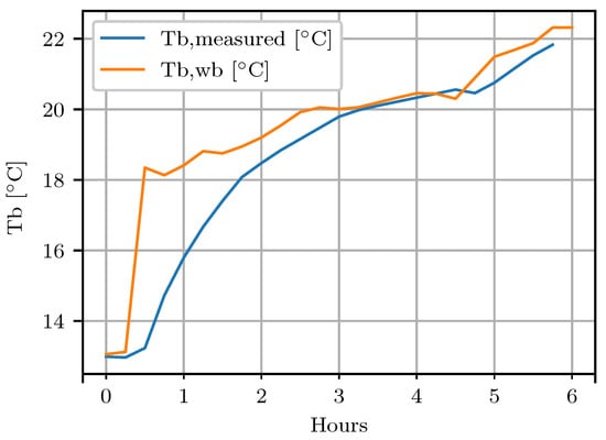
Figure 6.
Water basin temperature response for a fan state change.
To verify this observed behaviour, the black box model was used to simulate all 13 temperature transients due to fan state changes in the dataset. Figure 7 shows a box-plot, for both the first hour and first 6 h after the fan state change. Average RMSEs of 2.895 and 1.473 were obtained, respectively.
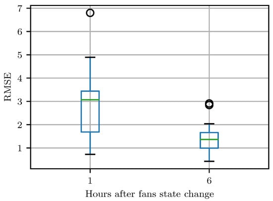
Figure 7.
Box-plot of the temperature response of 13 fan state changes.
This analysis shows that the black box model is well trained to simulate the water basin temperature in general, with an RMSE of 0.879, but it cannot simulate the temperature transients due to fan state changes with the same accuracy. The reason for this might be that, even though the model is trained with a large dataset (22,832 rows), only 13 fan state changes are included. Increasing the accuracy of the black box model on this particular aspect could be done by training the model with a dataset containing more fan state changes. In practice, this means the industrial sites cooling system operation should be adapted to obtain these data. This can be seen as a major drawback in using the black box method.
3.2. White Box
The development of an induced draft evaporative cooling tower model using a white box modelling approach is well described in the literature. Already in 1925, Merkel [12] pioneered in developing a thermal evaluation model for a cooling tower. Several assumptions are taken for granted in this theory; the air leaving the cooling tower is assumed to be saturated with water vapour, the reduction of water flow rate of evaporation is neglected and the Lewis factor (), relating the relative rates of heat and mass transfer, is considered to be 1. In the early 1970s, Poppe and Rogener [13] developed the Poppe model, not taking the simplified assumptions made by Merkel for granted. Later, in 1989, Jaber and Webb [14] applied the Number of Transfer Units (NTU) method on counterflow and crossflow cooling towers, resulting in a simplified solution procedure. The NTU method, also referred to as effectiveness-NTU or e-NTU is based on defining the maximum possible heat transfer. Scientific papers dealing with cooling towers often refer to one of the previously mentioned methods. Kloppers et al. [15] made a cooling tower performance evaluation between the different methods and concluded that, if only the outlet water temperature is of interest, the less accurate Merkel and NTU approaches can be used. In this case, all the models predict practically identical water outlet temperatures [15]. In [5], Viljoen et al. investigated the dynamic modelling of an induced draft cooling tower including the heat exchangers, pumps and fans. They also made initial assumptions regarding the cooling tower model. Two important assumptions are that the air leaving the cooling tower is saturated with water, i.e., the air has a relative humidity of 100%, and that the total mass of the water in the basin has an equal temperature, i.e., that the heat is evenly distributed.
3.2.1. Prerequisites and Limitations
The development of a white box model requires a complete knowledge of the mathematical equations and system parameters describing the cooling process. As discussed in Section 3.2, various theories exist to model a cooling tower. As in this work we focus on the water basin temperature only, we make some simplifying assumptions, which are listed below.
- The air leaving the cooling tower is saturated with water vapour, i.e., RHl = 100%.
- The temperature of the air leaving the cooling, is equal to the sum of the water basin temperature and half of the design range (which is 9 , see Section 2.1.1).
- The process heat is considered an input parameter and is defined by Equation (1).
- The total volume of water in the basin has an equal temperature.
- The Lewis factor is considered to be 1.
The white box model was implemented in Python 3 in a Jupyter Notebook environment. The Python Data Analysis Library (Pandas), NumPy and Matplotlib libraries were used for data handling, computation and visualisation. All required data were extracted from the SCADA system at the industrial site (see Table 1), with the exception of the relative humidity (RHe) and ambient air pressure (). RHe and historical data were obtained from [16] with an interval of 30 min. Data from the SCADA system have an interval of 15 min. A simulation time step of 15 min was used.
3.2.2. Model Development
To implement the white box modelling method, thermodynamic equations are used to model the working of the cooling tower, based on the laws of heat and mass conservation. The used model parameters and abbreviations are shown in Table 2, as well as the values for constants.
Table 2.
Model parameters.
The enthalpy of the entering and exiting air , together with the airflow through the cooling tower , define the cooling capacity . Including the process heat and the total volume of cooling water yields the increment or decrement of the cooling water temperature . The enthalpy of the air is calculated using empirical formulas according to the method presented by Ciprian [17], with the air temperature , water vapour saturation pressure , ambient air pressure and relative humidity RH as input parameters. First, the water vapour saturation pressure is calculated using the revised Arden Buck Equation (2) or Equation (3), for positive and negative dry bulb temperatures, respectively [18]. Next, the humidity ratio w is computed with Equation (4). The enthalpy of the moist air is then found using Equation (5).
The airflow through the cooling tower is related to the electric power supplied to the cooling tower fans [8]. The relation between the supplied electric power and the generated airflow is given by Equation (6) which was used by Panjeshahi et al. [19]. Rewriting the formula to obtain the airflow results in Equation (7). Needed parameters are the air density , frontal tower area , fan casing area , fan efficiency , motor efficiency and eliminator coefficient .
The fan efficiency can be determined by using Equation (8), for which the total pressure drop in the cooling tower and the specific fan power (SFP) are required. The SFP is defined by Equation (9) and the by Equation (10). The total pressure drop in the cooling tower is defined by the pressure drop over the fill and the miscellaneous pressure drop, given by Equation (11) [20].
The value for the pressure drop over the fill is 107.1 Pa, as read from the chart of the manufacturer [21]. When using the above formulas with the values in Table 2 and for operation in high speed mode, a fan efficiency of 0.558 is obtained. Note that this is the efficiency for the fan, starting from the mechanical shaft power. Including the motor efficiency of 0.946 for the high speed mode, as defined in Section 2.1, a total efficiency of 0.527 is obtained. This total efficiency may be low, considering the AMCA Standard 205 [22] with a threshold of 65%. Note that the cooling system at the INEOS industrial site has been commissioned in 1995 and the AMCA Standard 205 has been issued in 2011, hence the result of a lower total efficiency.
Using Equation (5) with both the entering and leaving air parameters combined with Equation (7), the cooling capacity of the tower is obtained by using Equation (12). The basin temperature change is found by using Equation (13). The water basin temperature at time t is found by summing the temperature at with the increment or decrement in temperature during , calculated with Equation (14).
3.2.3. Analysis
As in Section 3.1.3, an analysis is done on the temperature responses to fan state changes. Figure 8 shows the water basin temperature response, during the same period of 6 h starting from the fan state change as in Section 3.1.3. The black box curve is presented as well for comparison. The RMSE for the water basin temperature response of the white box model results in 0.256 for the first hour and 0.178 for the first 6 h. This specific fan switching is visualised to show the differences between the white box and black box temperature response. To verify the observed behaviour, i.e. the white box model is more accurate in simulating temperature responses to fan switches, all 13 fan switches (identical to the analysis in Section 3.1.3) were simulated and visualised. Figure 9 shows a box-plot for both the first hour and first 6 h after the fan state change. Average RMSEs of 1.513 and 0.998 were obtained, respectively.
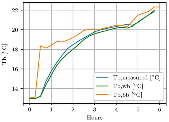
Figure 8.
Water basin temperature response for a fan state change.
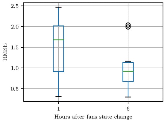
Figure 9.
Box-plot of the temperature responses of all fan state changes.
3.3. Model Comparison
In Section 3.1.3 and Section 3.2.3, the model accuracy on fan state changes is shown. For completeness, a fourteen-day period was also envisaged. The basin temperature was simulated during these fourteen days, with both models. At the start of the period, the measured basin temperature was set as starting point for the simulation. From then on forward, the basin temperature was only defined by the model’s calculated ; no synchronisation with measured data was executed. During the windowed time period, three different cooling system states were used. From the start of the simulation until Day 3 at 09:15 one fan was operated at high speed. Next, as the basin temperature was lower than necessary for the process, the active fan was shut down. The cooling system was now operating without active fans. On Day 12 at 16:00, both fans were activated to run at high speed, resulting in a basin temperature drop.
Figure 10 shows a time series plot of both the measured and simulated basin temperatures and for, respectively, the white box and black box modelling methods, during the complete windowed time period. For both models, the RMSE was calculated for the fourteen-day period, resulting in 0.445 and 0.570 for the white box and black box models, respectively. Table 3 gives an overview of the obtained RMSEs for the different evaluated timings.
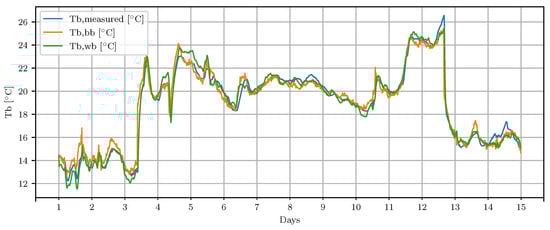
Figure 10.
Time series plot of the measured and simulated basin temperature, for the white box model (Tb,wb) and the black box model (Tb,bb).
Table 3.
Model accuracy comparison.
The engineering effort for both methods is different. The white box method requires quite extensive research towards the physics of evaporative cooling and investigation of the particular industrial cooling system parameters. For the black box method, the MATLAB ANFIS toolbox is used with the dataset containing the five inputs and one output. Very little knowledge of the system is needed and no parameters, dimensions or efficiencies of the particular industrial system are required. Another important difference is the applicability of both constructed models. While the black box model is system specific, the white box model is generic. Inputting the parameters of a different cooling system to the white box model would result in a direct usable simulation tool. Applying the black box model to another cooling system would require a new iteration of the training and testing, i.e., constructing a completely new model. It can be stated that both methods have their advantages and disadvantages and it should be carefully considered which approach to use, keeping in mind the desired applicability. As a final note, it should be stated that both models are developed with the idea of achieving an as high as possible accuracy while keeping the required data and information level as low as possible, to foster the easy implementation in an industrial setting. Accuracy of both models could be enhanced, but would result in a higher degree of complexity, dataset requirements and computing power.
4. Discussion on the Optimal Design and Operation Strategy
Considering the purpose of the developed models, defining the electrical flexibility of the cooling tower system, this section covers the topics of thermal mass and pre-cooling. Both are discussed in the light of “design for flexibility” and “operation for flexibility”, respectively.
4.1. Thermal Mass
As shown Section 3.1 and Section 3.2, we designed and applied the model on the existing forced draft evaporative cooling system available at the INEOS industrial site. The black box method is limited in use to existing systems as historical data are needed to develop the model. For the generic white box model, this is not the case. When designing a new or adapting an existing cooling system, it might be interesting to take into account the electrical flexibility the system can offer, i.e., designing for flexibility. Referring to [4], the induced draft evaporative cooling system is of interest for supplying DSR as it has a large thermal time constant. In this section, the white box model is used to check the influence of the total water volume on the thermal time constant of the cooling system. The thermal time constant or time constant for the thermal response of the system is defined as the time required to change 63.2% of the total difference between the initial and final temperature when subjected to fan state change. In [23], the thermal time constant is defined by Equation (15). The thermal time constant is proportional to the total heat storing mass in the system and inversely proportional to the heat conductance G.
According to Equation (15), the thermal time constant can be enlarged by decreasing the heat conductance G or increasing the mass in the system , i.e., the water volume. As the goal of the cooling system is to evacuate heat, decreasing the heat conductance is not desirable. The other possibility is to increase the mass of the system. Applying this on an induced draft evaporative cooling system, this translates into a larger basin and volume of water.
Figure 11 shows the simulated water basin temperatures for different water volumes in the cooling system for a period of 14 h. The blue curve is shown as reference with = 900 m3, in Simulations 1–6, is 450 m3, 1800 m3, 3600 m3, 5400 m3, 7200 m3 and 9000 m3, respectively. In Table 4, the thermal time constants are given for each simulation. To define the thermal time constant, the initial conditions, i.e., the process heat and weather influences of the system at Hour 0, were fixed for the rest of the simulation. In this way, a steady state temperature could be reached to calculate the thermal time constant. The thermal time constant increase due to the thermal mass enlargement was validated by the simulations. Following Equation (16), the time constant was doubled when doubling the thermal mass .
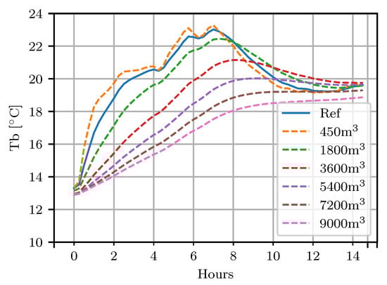
Figure 11.
The effect of water volume on the water basin temperature.
Table 4.
Thermal time constants for the basin enlarging simulation.
Considering the cooling systems flexibility potential, increasing the total water volume and applying the technique of pre-cooling can both be useful to lower the reached maximum temperatures and increase the timeframe in which the fans can be controlled without exceeding Tmax or Tmin.
4.2. Pre-Cooling
As discussed in Section 1 and shown in Figure 1, a temperature range is present for operating an induced draft evaporative cooling system. The maximum temperature Tmax cannot be exceeded with respect to process efficiency and safety. When considering the use of the cooling system for DSR purposes, it can be beneficial to increase the length of power consumption reduction, without exceeding Tmax. In this section, the concept of pre-cooling is laid out. The idea of pre-cooling is straightforward; the temperature of a certain medium is lowered before a period of temperature increase. The uttermost used reason for applying pre-cooling in combination with a “switch off period” is electricity peak consumption avoidance and the associated cost savings while keeping the temperature within the preset boundaries [24,25,26]. In the doctoral dissertation of P. Romanos [27], pre-cooling is investigated for buildings. P. Romanos concluded that the pre-cooling period is independent from the temperature reduction, has a certain maximum duration and that the duration of the “switch off period" is dependent on the pre-cooling period.
Figure 12 shows the water basin temperature curve for 10 h. The blue curve is shown as reference, no fan state changes occur and one fan is active at high speed, i.e., = 89.73 kW. The first simulation showed the temperature curve in the case the active fan is shutdown for one hour (03:45–04:45) without pre-cooling. To limit the resulting temperature spike from Simulation 1, pre-cooling was applied in Simulations 2–6 with durations of 15 min, 30 min, 1 h, 2 h and 3 h, respectively. During pre-cooling, both fans were switched to high speed, i.e., = 179.46 kW. Table 5 shows the reached maximum temperatures for each simulation.
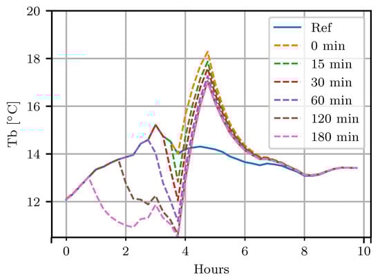
Figure 12.
The effect of pre-cooling on the water basin temperature.
Table 5.
Reached maximum temperatures for the pre-cooling simulations.
The reached maximum temperatures show that the beneficial duration of the pre-cooling period is limited, as also shown by Romanos [27]. Longer pre-cooling would only lead to extra power consumption without benefits towards maximum temperature. It can be concluded that, for this specific case, a pre-cooling time of 200% (2 h of pre-cooling for a switch-off period of 1 h) is considered the limited beneficial time. A temperature spike reduction of 1.23 is obtained. Note that, while pre-cooling might be beneficial to elongate the duration of the switch-off period, fostering the DSR purpose of the cooling system, an increase of total energy consumption is observed.
5. Conclusions
This article shows two modelling methods for an induced draft evaporative cooling tower. The cooling tower model is developed for the purpose of defining the electrical flexibility of the system, using the water basin temperature as limiting factor. First, in Section 3.1, a black box model, based on an Adaptive Neuro-Fuzzy Interference System, is developed with the data from an INEOS industrial site in Belgium. A total of five input parameters are used and the model is trained and optimised, obtaining an RMSE for the water basin temperature of 0.879 for the testing dataset. Considering the model purpose, attention is given to the temperature responses for fan state changes. A total of 13 temperature responses to fan state changes, as present in the dataset, were simulated. The RMSE was calculated for the first hour and first six hours after the fan state change. RMSEs of 2.895 and 1.473 were obtained, respectively. A white box modelling approach was applied as well, resulting in a thermodynamic model of the cooling system. An identical analysis was carried out on the fan state changes in the dataset, resulting in RMSEs of 1.513 and 0.998, respectively. For model analysis completeness, a four-teen day period was also envisaged, during which both the white box and black box model were used to simulate the water basin temperature. RMSEs of 0.445 and 0.570 were obtained for the white box and black box methods, respectively. Comparing both models, the overall accuracy was considered comparable. Looking at the accuracy for the fan state changes, the white box model performed better than the black box model. The main reason is the limited number of fan state changes which occur in the dataset used to construct the black box model. We can conclude that, when simulating the water basin temperature for DSR purposes, i.e., when temperature responses to fan state changes are of importance, the white box model will give more correct results. Considering forced draft evaporative cooling systems in design or adaptation phase, the concept of design for flexibility is touched upon discussing the impact of the total thermal mass in the cooling system. The white box model is used for simulations, the black box model is not suitable as it is developed and therefore valid for the cooling system at the INEOS industrial site only. The simulation results verify the proportionality between the time constant and the thermal mass .
The white box model was used to simulate the concept of pre-cooling, i.e., lowering the maximum reached temperature in a “switch off period" by increasing cooling capacity prior to this period. The beneficial period of pre-cooling is limited in time with respect to the reached maximum temperature. For a specific case, it was shown that a maximum pre-cooling time of 200% is still beneficial, resulting in a temperature spike reduction of 1.23 .
The cooling system could be considered as a thermal battery, with the goal of operating the fans in an electrically flexible way, i.e., for DSR purposes. The developed models allow estimating the water basin temperature, making it possible to simulate different fan switching algorithms. By applying the pre-cooling methodology or enlarging the water basin an even larger window is obtained for implementation of electrical flexibility algorithms. Future research will focus on the development of a fan switching algorithm, implementing the developed models for water basin temperature simulations.
Author Contributions
Conceptualization, J.B. and J.D.M.D.K.; Methodology, J.B. and N.K.; Resources, G.L.; Supervision, G.V.E., J.D.M.D.K. and L.V.; and Writing—original draft, J.B.
Funding
This research was funded by Flanders Innovation and Entrepreneurship (VLAIO), grant number HBC.2017.0361.
Acknowledgments
The work presented in this paper was carried out in the frame of the FLEX project. The authors acknowledge INEOS for the use of edited data from one of its chemical industry sites in Belgium.
Conflicts of Interest
The authors declare no conflict of interest.
References
- European Commission. The Commission Presents Strategy for a Climate Neutral Europe by 2050—Questions and Answers; European Commission: Brussels, Belgium, 2018. [Google Scholar]
- Baetens, J.; Zwaenepoel, B.; De Kooning, J.D.M.; Van Eetvelde, G.; Vandevelde, L. Thermal systems in process industry as a source for electrical flexibility. In Proceedings of the 52nd International Universities Power Engineering Conference (UPEC), Crete, Greece, 28–31 August 2017. [Google Scholar]
- Müller, T. The role of demand side management for the system integration of renewable energies. In Proceedings of the 14th International Conference on the European Energy Market (EEM), Dresden, Germany, 6–9 June 2017; pp. 1–6. [Google Scholar]
- Zwaenepoel, B.; Baetens, J.; Van Eetvelde, G.; Vandevelde, L. Assessing electrical flexibility in process industry. In Proceedings of the 7th International Conference & Workshop REMOO–2017, Venice, Italy, 10–12 May 2017. [Google Scholar]
- Viljoen, J.; Muller, C.; Craig, I. Dynamic modelling of induced draft cooling towers with parallel heat exchangers, pumps and cooling water network. J. Process Control 2018, 68, 34–51. [Google Scholar] [CrossRef]
- Marley Cooling Tower; INEOS Project, Technical Description, Internal Document INEOS; INEOS: London, UK, 1995.
- Hosoz, M.; Ertunc, H.; Bulgurcu, H. An adaptive neuro-fuzzy inference system model for predicting the performance of a refrigeration system with a cooling tower. Expert Syst. Appl. 2011, 38, 14148–14155. [Google Scholar] [CrossRef]
- Pan, T.H.; Shieh, S.S.; Jang, S.S.; Tseng, W.H.; Wu, C.W.; Ou, J.J. Statistical multi-model approach for performance assessment of cooling tower. Energy Convers. Manag. 2011, 52, 1377–1385. [Google Scholar] [CrossRef]
- Hathaway, R.J.; Bezdek, J.C. Local convergence of the fuzzy c-Means algorithms. Pattern Recognit. 1986, 19, 477–480. [Google Scholar] [CrossRef]
- Hamid Abdalla, E.A.; Nallagownden, P.; Mohd Nor, N.B.; Romlie, M.F.; Hassan, S.M. An Application of a Novel Technique for Assessing the Operating Performance of Existing Cooling Systems on a University Campus. Energies 2018, 11, 719. [Google Scholar] [CrossRef]
- Jang, J.S.R. Fuzzy Modeling Using Generalized Neural Networks and Kalman Filter Algorithm. In Proceedings of the Ninth National Conference on Artificial Intelligence, Anaheim, CA, USA, 14–19 July 1991; Volume 2, pp. 762–767. [Google Scholar]
- Merkel, F. Verdunstungskühlung, Volume 70, Forschungsarbeiten auf dem Gebiete des Ingenieurwesens; VDI-Verlag: Düsseldorf, Germany, 1925; pp. 123–128. [Google Scholar]
- Poppe, M.; Rögener, H. Berechnung von Rückkühlwerken; VDI-Wärmeatlas: Düsseldorf, Germany, 1991; pp. Mi 1–Mi 15. [Google Scholar]
- Jaber, H.L.; Webb, R. Design of Cooling Towers by the Effectiveness-NTU Method. J. Heat Transf.-Trans. ASME 1989, 111, 837–843. [Google Scholar] [CrossRef]
- Kloppers, J.C.; Kroöger, D.G. Cooling Tower Performance Evaluation: Merkel, Poppe, and e-NTU Methods of Analysis. J. Eng. Gas Turbines Power ASME 2005, 127, 1–7. [Google Scholar] [CrossRef]
- Past Weather. Available online: https://www.timeanddate.com/weather/ (accessed on 22 October 2018).
- Balan, M.; Mrenes, M.; Plesa, A. Simulation of the moist air thermodynamic properties. Acta Tech. Napoc. Sect. Constr. Mach. Mater. U.T. Cluj-Napoca 2001, 44, 133–138. [Google Scholar]
- Buck, L.A. New Equations for Computing Vapor Pressure and Enhancement Factor. J. Appl. Meteorol. 1981, 20, 1527–1532. [Google Scholar] [CrossRef]
- Panjeshahi, M.H.A.; Ataei, A.; Gharaie, M. A Comprehensive Approach to an Optimum Design and Simulation Model of a Mechanical Draft Wet Cooling Tower. Iran. J. Chem. Chem. Eng. (IJCCE) 2010, 29, 21–32. [Google Scholar]
- Rubio-Castro, E.; Serna-Gonzalez, M.; Ponce-Ortega, J.M.; Jimenez-Gutieerrez, A. Optimal Design of Cooling Towers; Heat and Mass Transfer—Modeling and Simulation; IntechOpen: Londen, UK, 2011. [Google Scholar]
- SPX Cooling Technologies, Inc. MC75 Film Fill Datasheet. 2018. Available online: https://spxcooling.com/parts/mc75-counterflow-film-fill (accessed on 7 May 2019).
- AMCA Standard 205-10, Rev. 2011. Energy Efficiency Classification for Fans. 2011. Available online: https://www.amca.org/assets/resources/public/userfiles/file/AMCA%20205-10%20(Rev_%202011).pdf (accessed on 7 May 2019).
- Hedbrandt, J. On the Thermal Inertia and Time Constant of Single-Family Houses. Ph.D. Thesis, Linkopings Universitet, Linkoping, Sweden, 2001. [Google Scholar]
- Yin, R.; Xu, P.; Piette, M.A.; Kiliccote, S. Study on Auto-DR and pre-cooling of commercial buildings with thermal mass in California. Energy Build. 2010, 42, 967–975. [Google Scholar] [CrossRef]
- Bhattacharya, S.; Kar, K.; Chow, J.H. Optimal precooling of thermostatic loads under time-varying electricity prices. In Proceedings of the 2017 American Control Conference (ACC), Seattle, WA, USA, 24–26 May 2017; pp. 1407–1412. [Google Scholar]
- Sun, Y.; Wang, S.; Xiao, L.; Huang, G. A Study of Pre-cooling Impacts on Peak Demand Limiting in Commercial Buildings. HVAC&R Res. 2012, 18. [Google Scholar] [CrossRef]
- Romanos, P. Thermal Model Predictive Control for Demand Side Management Cooling Strategies; Kassel University Press: Hessen, Germany, 2008. [Google Scholar]


© 2019 by the authors. Licensee MDPI, Basel, Switzerland. This article is an open access article distributed under the terms and conditions of the Creative Commons Attribution (CC BY) license (http://creativecommons.org/licenses/by/4.0/).