On the Use of the Harmonic Mean Estimator for Selecting the Hypothetical Income Distribution from Grouped Data

Abstract

It is known that the harmonic mean estimator is a consistent estimator of the marginal likelihood and is easy to implement, but it has severe biases and does not change as much as the prior distribution changes. In this study, we investigate the use of the harmonic mean estimator to select the hypothetical income distribution from grouped data through Monte Carlo simulations and apply it to real data in Japan. From the results, we confirm that there are significant biases, but it can be reliably used to select an appropriate model only when the sample size is large enough under appropriate prior settings.

1. Introduction

Non-negative statistical distributions and their applications are studied and used in areas such as finance (Higbee & McDonald, 2024), among others. One such example is the work of Professor Chris Heyde; see, for example, Heyde (1964, 1986). Among them, income distribution is widely considered to be one of the most important research areas involving non-negative-valued random variables, and such distributions are relevant to societal outcomes in general. In estimating an income distribution, the choice of the initial hypothetical income distribution is a crucial consideration. However, we face a trade-off between fitting a precise hypothetical income distribution and the interpretability of the parameters. Therefore, in empirical studies, we often start with distributions such as the lognormal (LN) distribution, the Dagum (DA) distribution introduced by Dagum (1977), the Singh–Maddala (SM) distribution proposed by Singh and Maddala (1976), and others. These distributions are preferred for better interpretability of the parameters. In addition, the estimation of the more flexible generalized beta distribution of the second kind (hereinafter referred to as GB2 distribution), introduced by McDonald (1984), is also examined within a Bayesian framework by Kakamu and Nishino (2019).

Several Bayesian model selection criteria exist for choosing the most appropriate hypothetical income distribution from a set of candidate distributions (see, for example, Ando (2010) for Bayesian model selection). Among these criteria, the marginal likelihood is a common choice for selecting the hypothetical income distribution, and various estimators have been proposed for its accurate estimation. Accurate estimation of the marginal likelihood is critical when dealing with Bayesian model averaging (BMA) or Bayes factor estimation. Inaccurate estimates can lead to inappropriate inference. Therefore, the precision of marginal likelihood estimators is extensively studied in the literature, with works such as Friel and Wyse (2012); Kass and Raftery (1995) providing valuable insights. On the other hand, the harmonic mean estimator introduced by Newton and Raftery (1994) is a consistent estimator of the marginal likelihood and is easy to implement. However, it has been criticized for its significant biases and limited responsiveness to changes in prior information. Consequently, its use in BMA or Bayes factor estimation is controversial. However, if the sole objective is to select an appropriate hypothetical income distribution, it remains unclear whether the harmonic mean estimator can effectively serve this purpose.

This study explores the application of the harmonic mean estimator in selecting a hypothetical income distribution from grouped data using Monte Carlo simulations. We also apply this estimator to real data from a Japanese case study. Our results confirm the presence of significant biases in the harmonic mean estimator. Nevertheless, it can prove valuable in selecting an appropriate model, but its effectiveness is significantly more pronounced when the sample size is sufficiently large under appropriate prior settings.

The remainder of this paper is organized as follows. In Section 2, we explain the method for selecting the hypothetical income distribution using marginal likelihoods from grouped data. In Section 3 we implement the Monte Carlo simulations. Section 4 examines the real data in Japan. Finally, brief conclusions are given in Section 5.

2. Selecting the Hypothetical Income Distribution

Income data are published as grouped data in many countries. In grouped data, suppose that the income units are grouped into K income classes, viz., $(x_{\left[0\right]},x_{\left[1\right]})$, $(x_{\left[1\right]},x_{\left[2\right]})$, …, $(x_{[K-1]},x_{\left[K\right]})$, with $x_{\left[0\right]}=0$ and $x_{\left[K\right]}\le \infty$: Let n be the total number of units and $n_k$ be the number of units in the interval $x_{[k-1]}$ and $x_{\left[k\right]}$ for $k=1,2,\dots ,K$ and therefore ${\displaystyle n=\sum _{k=1}^K{n}_k}$. There are two types of grouped data (see Eckernkemper & Gribisch, 2021) and we assume the type of quantile form in this study (see Nishino & Kakamu, 2011). From the grouped data, we assume the hypothetical distribution and estimate its parameters.

Let $\mathit{\theta }$ be a $d\times 1$ vector of parameters for the assumed hypothetical income distribution. Let $f\left(x\right|\mathit{\theta })$ and $F\left(x\right|\mathit{\theta })$ be the probability density function (PDF) and cumulative distribution function (CDF) of the hypothetical income distribution, respectively. Given the grouped data, ${\mathbf{x}}_{\left[K\right]}={(x_{\left[1\right]},x_{\left[2\right]},\dots ,x_{[K-1]})}^{\prime }$ and $\mathbf{n}={(n_1,n_2,\dots ,n_K)}^{\prime }$, the likelihood function based on the selected order statistics by Nishino and Kakamu (2011) is given as follows:

$$\begin{array}{c}{\displaystyle L\left({\mathbf{x}}_{\left[K\right]}\right|\mathit{\theta },\mathbf{n})=n!\frac{{\displaystyle F{\left(x_{\left[1\right]}\right|\mathit{\theta })}^{n_1-1}}}{{\displaystyle (n_1-1)!}}f\left(x_{\left[1\right]}\right|\mathit{\theta })}\hfill \\ \times \left\{{\displaystyle \prod _{k=2}^{K-1}\frac{{\displaystyle {\left(F\left(x_{\left[k\right]}\right|\mathit{\theta })-F\left(x_{[k-1]}\right|\mathit{\theta })\right)}^{n_k-1}}}{{\displaystyle (n_k-1)!}}f\left(x_{\left[k\right]}\right|\mathit{\theta })}\right\}{\displaystyle \frac{{\displaystyle {\left(1-F\left(x_{[K-1]}\right|\mathit{\theta })\right)}^{n_K}}}{{\displaystyle n_K!}}}.\end{array}$$

(1)

To proceed with the Bayesian analysis, we need to assume the prior distribution as $\pi \left(\mathit{\theta }\right)$. Given the likelihood function (1) and prior distribution $\pi \left(\mathit{\theta }\right)$, the posterior distribution is expressed as

$$\begin{array}{c}\hfill \pi \left(\mathit{\theta }\right|{\mathbf{x}}_{\left[K\right]},\mathbf{n})={\displaystyle \frac{\pi \left(\mathit{\theta }\right)L\left({\mathbf{x}}_{\left[K\right]}\right|\mathit{\theta },\mathbf{n})}{m\left({\mathbf{x}}_{\left[K\right]}\right|\mathbf{n})}}\propto \pi \left(\mathit{\theta }\right)L\left({\mathbf{x}}_{\left[K\right]}\right|\mathit{\theta },\mathbf{n}),\end{array}$$

where $m\left({\mathbf{x}}_{\left[K\right]}\right|\mathbf{n})$ is called the marginal likelihood and used as a criterion to select the hypothetical income distribution. Using the posterior distribution, posterior inference via the Markov chain Monte Carlo (MCMC) method is implemented. This procedure is explained in Appendix A. In this study, the LN, DA, and SM distributions, which are denoted by $\mathcal{LN}(\mu ,{\sigma }^2)$, $\mathcal{DA}(a,b,p)$, and $\mathcal{SM}(a,b,q)$, respectively, are assumed as hypothetical income distributions.1

In this study, we focus on the estimation of the marginal likelihood, which is estimated from the MCMC draws ${\left\{{\mathit{\theta }}^{\left(r\right)}\right\}}_{r=1}^R$. As is shown by Gelfand and Dey (1994), for any proper PDF $g\left(\mathit{\theta }\right)$,

$$\begin{array}{cc}\hfill {\displaystyle \frac{1}{m\left({\mathbf{x}}_{\left[K\right]}\right|\mathbf{n})}}& ={\displaystyle \frac{1}{m\left({\mathbf{x}}_{\left[K\right]}\right|\mathbf{n})}}{\int }_{\Theta }g\left(\mathit{\theta }\right)d\mathit{\theta }\hfill \\ \hfill & ={\int }_{\Theta }{\displaystyle \frac{g\left(\mathit{\theta }\right)}{\pi \left(\mathit{\theta }\right)L\left({\mathbf{x}}_{\left[K\right]}\right|\mathit{\theta },\mathbf{n})}}{\displaystyle \frac{\pi \left(\mathit{\theta }\right)L\left({\mathbf{x}}_{\left[K\right]}\right|\mathit{\theta },\mathbf{n})}{m\left({\mathbf{x}}_{\left[K\right]}\right|\mathbf{n})}}d\mathit{\theta }\hfill \\ \hfill & ={\int }_{\Theta }{\displaystyle \frac{g\left(\mathit{\theta }\right)}{\pi \left(\mathit{\theta }\right)L\left({\mathbf{x}}_{\left[K\right]}\right|\mathit{\theta },\mathbf{n})}}\pi \left(\mathit{\theta }\right|{\mathbf{x}}_{\left[K\right]},\mathbf{n})d\mathit{\theta }\hfill \end{array}$$

for any hypothetical income distribution. Therefore, using the MCMC draws, we can obtain the estimator of the marginal likelihood as follows:

$$\begin{array}{c}\hfill {\widehat{m}}_{\mathrm{GD}}\left({\mathbf{x}}_{\left[K\right]}\right|\mathbf{n})={\left[{\displaystyle \frac{1}{R}}\sum _{r=1}^R{\displaystyle \frac{g\left({\mathit{\theta }}^{\left(r\right)}\right)}{\pi \left({\mathit{\theta }}^{\left(r\right)}\right)L\left({\mathbf{x}}_{\left[K\right]}\right|{\mathit{\theta }}^{\left(r\right)},\mathbf{n})}}\right]}^{-1}.\end{array}$$

(2)

In Equation (2), the choice of $g\left(\mathit{\theta }\right)$ is important and we need to specify it. Two major approaches are the harmonic mean estimator by Newton and Raftery (1994) and modified harmonic mean estimator by Geweke (1999). If we set $g\left(\mathit{\theta }\right)=\pi \left(\mathit{\theta }\right)$, then it becomes the harmonic mean estimator by Newton and Raftery (1994) as follows:

$$\begin{array}{c}\hfill {\widehat{m}}_{\mathrm{NR}}\left({\mathbf{x}}_{\left[K\right]}\right|\mathbf{n})={\left[{\displaystyle \frac{1}{R}}\sum _{r=1}^R{\displaystyle \frac{1}{L\left({\mathbf{x}}_{\left[K\right]}\right|{\mathit{\theta }}^{\left(r\right)},\mathbf{n})}}\right]}^{-1}.\end{array}$$

(3)

It is a consistent estimator of the marginal likelihood and easy to implement. However, it is also known that its variance can go to infinity, since it contains the inverse of the likelihood function, and that the harmonic mean estimator will not change much as the prior changes, even though the marginal likelihood is very sensitive to changes in the prior distribution.

To overcome the severe downside to this estimator, Geweke (1999) proposed the modified harmonic mean estimator. It is calculated as follows:

$$\begin{array}{c}\hfill {\widehat{m}}_{\mathrm{G}}\left({\mathbf{x}}_{\left[K\right]}\right|\mathbf{n})={\left[{\displaystyle \frac{1}{R}}\sum _{r=1}^R{\displaystyle \frac{h\left({\mathit{\theta }}^{\left(r\right)}\right)}{\pi \left({\mathit{\theta }}^{\left(r\right)}\right)L\left({\mathbf{x}}_{\left[K\right]}\right|{\mathit{\theta }}^{\left(r\right)},\mathbf{n})}}\right]}^{-1},\end{array}$$

(4)

where $h\left({\mathit{\theta }}^{\left(r\right)}\right)$ is a truncated normal distribution as follows:

$$\begin{array}{c}\hfill h\left({\mathit{\theta }}^{\left(r\right)}\right)=P^{-1}{\left(2\pi \right)}^{-d/2}{\left|\widehat{\Sigma }\right|}^{-1/2}exp\left\{-{\displaystyle \frac{{({\mathit{\theta }}^{\left(r\right)}-\widehat{\mathit{\theta }})}^{\prime }{\widehat{\Sigma }}^{-1}({\mathit{\theta }}^{\left(r\right)}-\widehat{\mathit{\theta }})}{2}}\right\}\end{array}$$

where $\widehat{\mathit{\theta }}$ and $\widehat{\Sigma }$ are the sample mean and covariance matrix from ${\left\{{\mathit{\theta }}^{\left(r\right)}\right\}}_{r=1}^R$ and P is the normalizing constant, which satisfies ${\displaystyle {({\mathit{\theta }}^{\left(r\right)}-\widehat{\mathit{\theta }})}^{\prime }{\widehat{\Sigma }}^{-1}({\mathit{\theta }}^{\left(r\right)}-\widehat{\mathit{\theta }})\le {\chi }_{\alpha }^2\left(d\right)}$ and ${\chi }_{\alpha }^2\left(d\right)$ is the $\alpha$ quantile of the ${\chi }^2$ distribution with degrees of freedom d. This approach is popular and is used in the analyses of income distribution, for example, by Griffiths et al. (2005) for the purpose of the BMA.

Another approach is proposed by Chib (1995) and Chib and Jeliazkov (2001) for the Gibbs sampler and Metropolis–Hastings (MH) algorithm, respectively. Their idea is based on the basic marginal likelihood identity as follows:

$$\begin{array}{c}\hfill m\left({\mathbf{x}}_{\left[K\right]}\right|\mathbf{n})={\displaystyle \frac{\pi \left(\mathit{\theta }\right)L\left({\mathbf{x}}_{\left[K\right]}\right|\mathit{\theta },\mathbf{n})}{\pi \left(\mathit{\theta }\right|{\mathbf{x}}_{\left[K\right]},\mathbf{n})}}.\end{array}$$

At any point $\overline{\mathit{\theta }}$, which is, for example, the posterior mean, in the case of the MH algorithm, Chib and Jeliazkov (2001) showed that $\pi \left(\overline{\mathit{\theta }}\right|{\mathbf{x}}_{\left[K\right]},\mathbf{n})$ can be estimated as follows:

$$\begin{array}{c}\hfill \widehat{\pi }\left(\overline{\mathit{\theta }}\right|{\mathbf{x}}_{\left[K\right]},\mathbf{n})={\displaystyle \frac{R^{-1}{\sum }_{r=1}^R\alpha ({\mathit{\theta }}^{\left(r\right)},\overline{\mathit{\theta }})q({\mathit{\theta }}^{\left(r\right)},\overline{\mathit{\theta }})}{R^{-1}{\sum }_{r=1}^R\alpha (\overline{\mathit{\theta }},{\mathit{\theta }}^{\left(r\right)})}},\end{array}$$

where $q({\mathit{\theta }}^{\left(r\right)},\overline{\mathit{\theta }})$ is the PDF of the proposal distribution.

Using the quantity, the marginal likelihood can be calculated as follows:

$$\begin{array}{c}\hfill {\widehat{m}}_{\mathrm{CJ}}\left({\mathbf{x}}_{\left[K\right]}\right|\mathbf{n})={\displaystyle \frac{\pi \left(\overline{\mathit{\theta }}\right)L\left({\mathbf{x}}_{\left[K\right]}\right|\overline{\mathit{\theta }},\mathbf{n})}{\widehat{\pi }\left(\overline{\mathit{\theta }}\right|{\mathbf{x}}_{\left[K\right]},\mathbf{n})}}.\end{array}$$

(5)

From the number of citations which these articles have gained, it is clear that their approach is popular among practitioners.

As a final note to this section, we briefly discuss the properties of marginal likelihood estimators. All estimators are consistent but biased. The difference lies in the size of the biases and the computational procedures. From the point of view of biases, the harmonic mean estimator is highly sensitive to the values of the likelihood in low-probability regions, a few extreme samples can dominate the estimate, and outliers in the parameter space can significantly affect the estimation result, making the method less robust. The modified harmonic mean estimator is proposed to overcome the problem of the harmonic mean estimator, but it is known that the estimators have biases when estimating high-dimensional parameter models such as latent variable models (see Chan & Grant, 2015). Finally, for the estimator of Chib and Jeliazkov (2001), difficulties can arise when this method is applied to mixture models, hidden Markov models, and other models that give rise to label switching and parameter non-identifiability, and the bias in these estimates is reported in Chan and Eisenstat (2015). From a computational point of view, the harmonic mean estimator is the easiest method to implement. On the other hand, the method by Chib and Jeliazkov (2001) increases in computational complexity as the dimension of parameters increases. Moreover, implementation is more involved, especially for computing numerical standard errors of marginal likelihood estimates. For a more comprehensive review of marginal likelihood estimation, see Chan and Eisenstat (2015); Friel and Wyse (2012); Han and Carlin (2001).

Using these three estimators of the marginal likelihood, we examine the selection of the hypothetical income distribution through Monte Carlo simulations and apply it to real data in Japan. All the results reported here were generated using Ox 9.10 (macOS_64/Parallel) (see Doornik, 2013).

3. Simulation Studies

We now explain the setup for the Monte Carlo simulations. First, we set the number of observations as n = 1000, 10,000, and 100,000 to evaluate the effect of the number of observations. In addition, we assume the number of groups as decile ($K=10$).2 Given n and $K=10$, we consider two scenarios in which the true data generating processes (DGPs) follow the LN distribution and GB2 distribution3, denoted by $\mathcal{GB}\mathit{2}(a,b,p,q)$, and L samples of $x_{\left[k\right]}$ for $k=1,2,\dots ,K-1$ are generated. That is, we perform L simulation runs for these two distributions; in this section, L = 1000.

The simulation procedure is as follows:

(i)

Given the true DGP, we generate random numbers $x_i$s, $i=1,2,\dots ,n$ from the distribution.

(ii)

We sort the random numbers in ascending order and pick up $x_{\left[k\right]}=x_{n_k}$, where ${\displaystyle n_k=n\times \frac{k}{K}}$ for $k=1,2,\dots ,K-1$.

(iii)

Given ${\mathbf{x}}_{\left[K\right]}={(x_{\left[1\right]},x_{\left[2\right]},\dots ,x_{[K-1]})}^{\prime }$ and the hyper-parameters (${\mu }_0,{\tau }_0^2,{\nu }_0,{\lambda }_0$), we obtain the estimates and marginal likelihoods assuming the LN, DA, and SM distributions. In the MCMC procedure, we run a random walk MH (RWMH) algorithm, with 4000 iterations excluding the first 2000 iterations. For the modified harmonic mean estimator, $\alpha =0.5$, $0.75$ and $0.9$ are considered.

(iv)

We repeat (i)–(iii) L times, where L = 1000, as mentioned above.

(v)

From L marginal likelihoods, we count the distribution with the largest marginal likelihood.

In the first scenario, we assume the true DGP as the LN distribution with $\mu =1$ and ${\sigma }^2=0.5$ and examine the prior sensitivity. Therefore, we assume $({\mu }_0,{\tau }_0^2,{\nu }_0,{\lambda }_0)=(0,100,2,1)$, $(0,1,2,1)$, $(0,1000,2,1)$, $(0,100,0.01,0.01)$, $(0,100,20,10)$ for the LN distribution and the same hyper-parameters (${\nu }_0$, ${\lambda }_0$) with the LN distribution for the SM and DA distributions.4

In the second scenario, the purpose of the analysis is to analyze whether the true distribution can be properly selected and what selection is made when the true distribution is not included in the candidate distributions. Therefore, we assume the GB2 distribution with $(a,b,p,q)=(2,1,1.5,1)$, $(2,1,3,1)$, $(2,1,1,1.5)$, $(2,1,1,3)$, $(2,1,2.5,1.5)$, $(2,1,1.5,2.5)$, where the first two cases assume that the true distributions are the DA distributions, the second two cases assume the true distributions are the SM distributions, and last two cases assume that the true distributions are not included in the candidate distributions. It should be mentioned that, as shown by Kakamu (2016), the SM distributions are selected if $p<q$ and $p>1$, while the DA distributions are selected if $p>q$ and $q>1$, in terms of AIC.5 As the hyper-parameters, we set $({\mu }_0,{\tau }_0^2,{\nu }_0,{\lambda }_0)=(0,100,2,1)$ for all cases.

Table 1 displays the results of our Monte Carlo simulations, assuming the LN distribution. The results reveal that when the sample size n is sufficiently large, for example, n = 100,000, the LN distribution is consistently selected correctly across all estimators, regardless of the hyper-parameter choices. However, as the sample size n decreases, the choice of hyper-parameters begins to influence the selection of the hypothetical income distribution, particularly when using Equations (4) and (5). In cases where the prior for $\mu$ becomes diffuse, i.e., when ${\tau }_0^2$ is large, the DA or SM distributions are preferred over the LN distribution, even if the true DGP is the LN distribution. Moreover, when ${\nu }_0$ and ${\lambda }_0$ are large, the DA distribution is favored. It seems to be affected by the prior information when the sample size is not large enough, because it is well-known that biases of Equations (4) and (5) are relatively smaller than Equation (3). It is also consistent with the previous literature because the harmonic mean estimator will not change much as the prior changes. Therefore, it is worth noting that the use of the harmonic mean estimator should be criticized when the sample size is not large enough and/or when we assume some tight prior distribution.

Table 1. Monte Carlo results of the log of marginal likelihoods for the LN distribution.

	${\mathit{\mu }}_0=0$, ${\mathit{\tau }}_0^2=100$, ${\mathit{\nu }}_0=2$, ${\mathit{\lambda }}_0=1$
	n = 1000				n = 10,000				n = 100,000
	LN	DA	SM		LN	DA	SM		LN	DA	SM
Newton and Raftery (1994)	726	136	138		990	3	7		1000	0	0
Geweke (1999) ($\alpha =0.5$)	280	379	341		986	9	5		1000	0	0
Geweke (1999) ($\alpha =0.75$)	289	373	338		986	9	5		1000	0	0
Geweke (1999) ($\alpha =0.9$)	289	371	340		986	9	5		1000	0	0
Chib and Jeliazkov (2001)	322	362	316		988	7	5		1000	0	0
	${\mathit{\mu }}_{\mathbf{0}}=\mathbf{0}$, ${\mathit{\tau }}_{\mathbf{0}}^{\mathbf{2}}=\mathbf{1}$, ${\mathit{\nu }}_{\mathbf{0}}=\mathbf{2}$, ${\mathit{\lambda }}_{\mathbf{0}}=\mathbf{1}$
	n = 1000				n = 10,000				n = 100,000
	LN	DA	SM		LN	DA	SM		LN	DA	SM
Newton and Raftery (1994)	733	128	139		990	3	7		1000	0	0
Geweke (1999) ($\alpha =0.5$)	699	158	143		992	4	4		1000	0	0
Geweke (1999) ($\alpha =0.75$)	704	157	139		992	4	4		1000	0	0
Geweke (1999) ($\alpha =0.9$)	700	159	141		992	4	4		1000	0	0
Chib and Jeliazkov (2001)	708	152	140		993	3	4		1000	0	0
	${\mathit{\mu }}_{\mathbf{0}}=\mathbf{0}$, ${\mathit{\tau }}_{\mathbf{0}}^{\mathbf{2}}=$ 10,000, ${\mathit{\nu }}_{\mathbf{0}}=\mathbf{2}$, ${\mathit{\lambda }}_{\mathbf{0}}=\mathbf{1}$
	n = 1000				n = 10,000				n = 100,000
	LN	DA	SM		LN	DA	SM		LN	DA	SM
Newton and Raftery (1994)	742	128	130		988	4	8		1000	0	0
Geweke (1999) ($\alpha =0.5$)	10	508	482		971	19	10		1000	0	0
Geweke (1999) ($\alpha =0.75$)	15	508	477		971	19	10		1000	0	0
Geweke (1999) ($\alpha =0.9$)	14	513	473		971	19	10		1000	0	0
Chib and Jeliazkov (2001)	29	507	464		972	18	10		1000	0	0
	${\mathit{\mu }}_{\mathbf{0}}=\mathbf{0}$, ${\mathit{\tau }}_{\mathbf{0}}^{\mathbf{2}}=\mathbf{100}$, ${\mathit{\nu }}_{\mathbf{0}}=\mathbf{0.01}$, ${\mathit{\lambda }}_{\mathbf{0}}=\mathbf{0.01}$
	n = 1000				n = 10,000				n = 100,000
	LN	DA	SM		LN	DA	SM		LN	DA	SM
Newton and Raftery (1994)	740	145	115		988	6	6		1000	0	0
Geweke (1999) ($\alpha =0.5$)	999	0	1		1000	0	0		1000	0	0
Geweke (1999) ($\alpha =0.75$)	999	0	1		1000	0	0		1000	0	0
Geweke (1999) ($\alpha =0.9$)	999	0	1		1000	0	0		1000	0	0
Chib and Jeliazkov (2001)	998	0	2		999	1	0		1000	0	0
	${\mathit{\mu }}_{\mathbf{0}}=\mathbf{0}$, ${\mathit{\tau }}_{\mathbf{0}}^{\mathbf{2}}=\mathbf{100}$, ${\mathit{\nu }}_{\mathbf{0}}=\mathbf{20}$, ${\mathit{\lambda }}_{\mathbf{0}}=\mathbf{10}$
	n = 1000				n = 10,000				n = 100,000
	LN	DA	SM		LN	DA	SM		LN	DA	SM
Newton and Raftery (1994)	750	88	162		989	4	7		1000	0	0
Geweke (1999) ($\alpha =0.5$)	348	568	84		991	5	4		1000	0	0
Geweke (1999) ($\alpha =0.75$)	344	575	81		991	5	4		1000	0	0
Geweke (1999) ($\alpha =0.9$)	351	569	80		991	5	4		1000	0	0
Chib and Jeliazkov (2001)	390	538	72		991	5	4		1000	0	0

To investigate why the true distribution is not selected in small samples and under certain prior settings, we examined the empirical distributions of the log of marginal likelihoods and the posterior means from the LN, DA, and SM distributions. Table 2 presents the means and standard deviations of the log of marginal likelihoods obtained from Monte Carlo simulations. The results reveal the following: First, the distribution with the highest mean marginal likelihood was consistently selected. Second, the means reported by Geweke (1999) and Chib and Jeliazkov (2001) are similar, whereas those of Newton and Raftery (1994) differ from Geweke (1999) and Chib and Jeliazkov (2001) across all cases. Third, when n = 1000, the marginal likelihood estimates appear relatively stable for Newton and Raftery (1994). However, these estimates change when ${\tau }_0^2$ is altered or when ${\nu }_0$ and ${\lambda }_0$ are adjusted. In particular, the changes in the marginal likelihood estimates for LN, when ${\nu }_0$ and ${\lambda }_0$ are varied, indicate greater sensitivity to the choice of hyper-parameters compared to changes in ${\tau }_0^2$. Needless to say, the marginal likelihood estimates are even more sensitive to the choice of hyper-parameters in Geweke (1999) and Chib and Jeliazkov (2001). Based on these observations, we proceed to examine the posterior estimates derived from the three distributions.

Table 2. Summary statistics of the log of marginal likelihoods for the LN distribution.

	${\mathit{\mu }}_0=0$, ${\mathit{\tau }}_0^2=100$, ${\mathit{\nu }}_0=2$, ${\mathit{\lambda }}_0=1$
	n = 1000				n = 10,000				n = 100,000
	LN	DA	SM		LN	DA	SM		LN	DA	SM
Newton and Raftery (1994)	11.771	10.242	10.224		22.071	8.905	8.924		32.519	−92.521	−92.283
	(2.037)	(2.314)	(2.299)		(2.066)	(5.411)	(5.393)		(1.977)	(15.708)	(15.742)
Geweke (1999) ($\alpha =0.5$)	3.894	4.581	4.516		11.882	0.029	0.011		20.015	−104.840	−104.681
	(1.893)	(2.219)	(2.161)		(1.946)	(5.350)	(5.304)		(1.826)	(15.629)	(15.754)
Geweke (1999) ($\alpha =0.75$)	3.889	4.564	4.504		11.879	0.022	0.002		20.014	−104.849	−104.689
	(1.892)	(2.219)	(2.158)		(1.945)	(5.353)	(5.304)		(1.823)	(15.630)	(15.752)
Geweke (1999) ($\alpha =0.9$)	3.886	4.555	4.497		11.877	0.016	−0.007		20.012	−104.856	−104.697
	(1.893)	(2.219)	(2.158)		(1.945)	(5.352)	(5.303)		(1.823)	(15.630)	(15.753)
Chib and Jeliazkov (2001)	4.103	4.571	4.449		12.084	−0.043	−0.066		20.215	−104.904	−104.756
	(1.926)	(2.277)	(2.213)		(1.992)	(5.357)	(5.306)		(1.865)	(15.652)	(15.739)
	${\mathit{\mu }}_{\mathbf{0}}=\mathbf{0}$, ${\mathit{\tau }}_{\mathbf{0}}^{\mathbf{2}}=\mathbf{1}$, ${\mathit{\nu }}_{\mathbf{0}}=\mathbf{2}$, ${\mathit{\lambda }}_{\mathbf{0}}=\mathbf{1}$
	n = 1000				n = 10,000				n = 100,000
	LN	DA	SM		LN	DA	SM		LN	DA	SM
Newton and Raftery (1994)	11.800	10.242	10.224		22.069	8.905	8.924		32.560	−92.521	−92.283
	(1.989)	(2.314)	(2.299)		(2.035)	(5.411)	(5.393)		(1.962)	(15.708)	(15.742)
Geweke (1999) ($\alpha =0.5$)	5.698	4.581	4.516		13.692	0.029	0.011		21.823	−104.840	−104.681
	(1.897)	(2.219)	(2.161)		(1.950)	(5.350)	(5.304)		(1.823)	(15.629)	(15.754)
Geweke (1999) ($\alpha =0.75$)	5.698	4.564	4.504		13.687	0.022	0.002		21.822	−104.849	−104.689
	(1.896)	(2.219)	(2.158)		(1.949)	(5.353)	(5.304)		(1.823)	(15.630)	(15.752)
Geweke (1999) ($\alpha =0.9$)	5.694	4.555	4.497		13.685	0.016	−0.007		21.819	−104.856	−104.697
	(1.896)	(2.219)	(2.158)		(1.949)	(5.352)	(5.303)		(1.822)	(15.630)	(15.753)
Chib and Jeliazkov (2001)	5.911	4.571	4.449		13.911	−0.043	−0.066		22.039	−104.904	−104.756
	(1.936)	(2.277)	(2.213)		(2.025)	(5.357)	(5.306)		(1.858)	(15.652)	(15.739)
	${\mathit{\mu }}_{\mathbf{0}}=\mathbf{0}$, ${\mathit{\tau }}_{\mathbf{0}}^{\mathbf{2}}=$ 10,000, ${\mathit{\nu }}_{\mathbf{0}}=\mathbf{2}$, ${\mathit{\lambda }}_{\mathbf{0}}=\mathbf{1}$
	n = 1000				n = 10,000				n = 100,000
	LN	DA	SM		LN	DA	SM		LN	DA	SM
Newton and Raftery (1994)	11.797	10.242	10.224		22.099	8.905	8.924		32.567	−92.521	−92.283
	(2.023)	(2.314)	(2.299)		(2.051)	(5.411)	(5.393)		(1.945)	(15.708)	(15.742)
Geweke (1999) ($\alpha =0.5$)	1.594	4.581	4.516		9.585	0.029	0.011		17.720	−104.840	−104.681
	(1.895)	(2.219)	(2.161)		(1.945)	(5.350)	(5.304)		(1.824)	(15.629)	(15.754)
Geweke (1999) ($\alpha =0.75$)	1.591	4.564	4.504		9.581	0.022	0.002		17.716	−104.849	−104.689
	(1.894)	(2.219)	(2.158)		(1.945)	(5.353)	(5.304)		(1.823)	(15.630)	(15.752)
Geweke (1999) ($\alpha =0.9$)	1.590	4.555	4.497		9.579	0.016	−0.007		17.713	−104.856	−104.697
	(1.893)	(2.219)	(2.158)		(1.945)	(5.352)	(5.303)		(1.823)	(15.630)	(15.753)
Chib and Jeliazkov (2001)	1.804	4.571	4.449		9.783	−0.043	−0.066		17.937	−104.904	−104.756
	(1.935)	(2.277)	(2.213)		(1.977)	(5.357)	(5.306)		(1.864)	(15.652)	(15.739)
	${\mathit{\mu }}_{\mathbf{0}}=\mathbf{0}$, ${\mathit{\tau }}_{\mathbf{0}}^{\mathbf{2}}=\mathbf{100}$, ${\mathit{\nu }}_{\mathbf{0}}=\mathbf{0.01}$, ${\mathit{\lambda }}_{\mathbf{0}}=\mathbf{0.01}$
	n = 1000				n = 10,000				n = 100,000
	LN	DA	SM		LN	DA	SM		LN	DA	SM
Newton and Raftery (1994)	11.778	10.211	10.114		22.097	8.942	8.961		32.531	−92.485	−92.298
	(2.026)	(2.364)	(2.320)		(2.063)	(5.392)	(5.377)		(1.869)	(15.638)	(15.769)
Geweke (1999) ($\alpha =0.5$)	−0.149	−7.093	−7.048		7.838	−11.643	−11.626		15.976	−116.513	−116.319
	(1.894)	(2.191)	(2.161)		(1.945)	(5.351)	(5.307)		(1.823)	(15.636)	(15.750)
Geweke (1999) ($\alpha =0.75$)	−0.149	−7.113	−7.059		7.835	−11.653	−11.634		15.970	−116.522	−116.327
	(1.891)	(2.189)	(2.162)		(1.945)	(5.351)	(5.306)		(1.822)	(15.637)	(15.750)
Geweke (1999) ($\alpha =0.9$)	−0.153	−7.118	−7.066		7.834	−11.660	−11.641		15.967	−116.529	−116.336
	(1.891)	(2.194)	(2.163)		(1.946)	(5.350)	(5.308)		(1.822)	(15.636)	(15.752)
Chib and Jeliazkov (2001)	0.056	−7.131	−7.095		8.054	−11.736	−11.692		16.180	−116.597	−116.387
	(1.954)	(2.213)	(2.215)		(1.989)	(5.378)	(5.338)		(1.860)	(15.681)	(15.759)
	${\mathit{\mu }}_{\mathbf{0}}=\mathbf{0}$, ${\mathit{\tau }}_{\mathbf{0}}^{\mathbf{2}}=\mathbf{100}$, ${\mathit{\nu }}_{\mathbf{0}}=\mathbf{20}$, ${\mathit{\lambda }}_{\mathbf{0}}=\mathbf{10}$
	n = 1000				n = 10,000				n = 100,000
	LN	DA	SM		LN	DA	SM		LN	DA	SM
Newton and Raftery (1994)	11.864	9.169	10.227		22.096	7.963	8.893		32.558	−92.636	−92.303
	(1.969)	(2.566)	(2.324)		(2.062)	(5.534)	(5.359)		(1.894)	(15.653)	(15.745)
Geweke (1999) ($\alpha =0.5$)	5.037	5.689	3.389		13.068	−0.238	−0.923		21.206	−105.418	−105.596
	(1.898)	(2.762)	(2.266)		(1.947)	(5.414)	(5.297)		(1.819)	(15.620)	(15.750)
Geweke (1999) ($\alpha =0.75$)	5.033	5.675	3.379		13.064	−0.248	−0.931		21.204	−105.426	−105.604
	(1.897)	(2.758)	(2.266)		(1.947)	(5.415)	(5.296)		(1.822)	(15.618)	(15.751)
Geweke (1999) ($\alpha =0.9$)	5.028	5.668	3.368		13.060	−0.255	−0.936		21.200	−105.433	−105.612
	(1.896)	(2.758)	(2.264)		(1.947)	(5.415)	(5.294)		(1.822)	(15.617)	(15.750)
Chib and Jeliazkov (2001)	5.252	5.785	3.293		13.266	−0.317	−0.991		21.423	−105.528	−105.689
	(1.929)	(2.762)	(2.321)		(1.964)	(5.408)	(5.317)		(1.873)	(15.637)	(15.755)

Table 3, Table 4 and Table 5 present summaries of the empirical distributions of the posterior means derived from the LN, DA, and SM distributions. The means and standard deviations of the posterior means from the LN distribution (see Table 3) exhibit minimal variation, whereas those from the DA and SM distributions (see Table 4 and Table 5) show noticeable changes, particularly when the sample size is small (n = 1000). Additionally, it is noteworthy that the influence of the prior settings persists even when the sample size increases to n = 100,000 (e.g., for ${\nu }_0=20$ and ${\lambda }_0=10$). This indicates that the choice of hyper-parameters affects the posterior estimates of the hypothetical income distribution, leading to variations in the marginal likelihood estimates, particularly for Chib and Jeliazkov (2001); Geweke (1999).

Table 3. Summary statistics of the LN distribution.

Hyper-Parameters	n = 1000			n = 10,000			n = 100,000
	$\mathit{\mu }$	${\mathit{\sigma }}^2$		$\mathit{\mu }$	${\mathit{\sigma }}^2$		$\mathit{\mu }$	${\mathit{\sigma }}^2$
${\mu }_0=0$, ${\tau }_0^2=100$,	1.000	0.504		1.000	0.501		1.000	0.500
${\nu }_0=2$, ${\lambda }_0=1$	(0.023)	(0.027)		(0.007)	(0.009)		(0.002)	(0.003)
${\mu }_0=0$, ${\tau }_0^2=1$,	0.999	0.504		1.000	0.501		1.000	0.500
${\nu }_0=2$, ${\lambda }_0=1$	(0.023)	(0.027)		(0.007)	(0.009)		(0.002)	(0.003)
${\mu }_0=0$, ${\tau }_0^2=$ 10,000,	1.000	0.504		1.000	0.501		1.000	0.500
${\nu }_0=2$, ${\lambda }_0=1$	(0.023)	(0.027)		(0.007)	(0.009)		(0.002)	(0.003)
${\mu }_0=0$, ${\tau }_0^2=100$,	1.000	0.504		1.000	0.501		1.000	0.500
${\nu }_0=0.01$, ${\lambda }_0=0.01$	(0.023)	(0.027)		(0.007)	(0.009)		(0.002)	(0.003)
${\mu }_0=0$, ${\tau }_0^2=100$,	1.000	0.503		1.000	0.501		1.000	0.500
${\nu }_0=20$, ${\lambda }_0=10$	(0.023)	(0.025)		(0.007)	(0.009)		(0.002)	(0.003)

Note: The means and standard deviations (in parentheses) of the empirical distribution of the posterior means from the LN distribution are displayed when the true DGPs are from the LN distribution.

Table 4. Summary statistics of the DA distribution.

Hyper-Parameters	n = 1000				n = 10,000				n = 100,000
	a	b	p		a	b	p		a	b	p
${\nu }_0=2$, ${\lambda }_0=1$	2.316	2.538	1.169		2.343	2.640	1.052		2.348	2.653	1.040
	(0.148)	(0.309)	(0.233)		(0.047)	(0.100)	(0.060)		(0.015)	(0.032)	(0.018)
${\nu }_0=0.01$, ${\lambda }_0=0.01$	2.350	2.610	1.124		2.347	2.648	1.047		2.348	2.654	1.040
	(0.159)	(0.329)	(0.247)		(0.047)	(0.101)	(0.060)		(0.015)	(0.032)	(0.018)
${\nu }_0=20$, ${\lambda }_0=10$	2.149	2.160	1.451		2.310	2.566	1.099		2.344	2.645	1.045
	(0.084)	(0.179)	(0.173)		(0.044)	(0.096)	(0.061)		(0.015)	(0.032)	(0.019)

Note: The means and standard deviations (in parentheses) of the empirical distribution of the posterior means from the DA distribution are displayed when the true DGPs are from the LN distribution.

Table 5. Summary statistics of the SM distribution.

Hyper-Parameters	n = 1000				n = 10,000				n = 100,000
	a	b	p		a	b	p		a	b	p
${\nu }_0=2$, ${\lambda }_0=1$	2.342	2.928	1.128		2.345	2.804	1.050		2.347	2.790	1.042
	(0.144)	(0.364)	(0.212)		(0.048)	(0.107)	(0.060)		(0.015)	(0.033)	(0.018)
${\nu }_0=0.01$, ${\lambda }_0=0.01$	2.352	2.927	1.127		2.347	2.800	1.048		2.347	2.790	1.041
	(0.158)	(0.429)	(0.256)		(0.048)	(0.108)	(0.060)		(0.015)	(0.033)	(0.018)
${\nu }_0=20$, ${\lambda }_0=10$	2.280	2.993	1.173		2.332	2.830	1.066		2.345	2.793	1.043
	(0.085)	(0.201)	(0.114)		(0.045)	(0.102)	(0.057)		(0.015)	(0.033)	(0.018)

Note: The means and standard deviations (in parentheses) of the empirical distribution of the posterior means from the SM distribution are displayed when the true DGPs are from the LN distribution.

To sum up, when the sample size is sufficiently large, the posterior estimates of the LN, DA, and SA do not change and the weight of the prior distribution seems to be sufficiently small (see Table 3, Table 4 and Table 5). Therefore, the marginal likelihood estimates of Newton and Raftery (1994), Geweke (1999), and Chib (1995) do not change, even when the hyper-parameters have changed (see Table 2). On the other hand, the posterior estimates of the DA and SM distributions are different when the hyper-parameters have changed (see Table 4 and Table 5), but the posterior estimates of the LN distribution, especially the ones of ${\sigma }^2$, have small biases; however, the biases do not change so much, even when the hyper-parameters have changed (see Table 3). Moreover, the marginal likelihood estimates of Geweke (1999) and Chib (1995) require prior distribution to estimate them. We think these facts lead to small changes in the marginal likelihoods of Geweke (1999) and Chib (1995) and the wrong choice of hypothetical income distribution depending on the hyper-parameter settings (see Table 2). These results suggest that selecting appropriate hyper-parameters is crucial, especially when the sample size is small. However, with a sufficiently large sample size and appropriate prior settings, valid model selection can still be achieved.

Table 6 presents the results of our Monte Carlo simulations under the assumption of the GB2 distribution. Similar to the findings under the LN distribution, when the sample size n is sufficiently large, for instance, n = 100,000, the true distribution is consistently favored, aligning with Kakamu (2016), even when the true distributions are not included among the candidate distributions. However, as the sample size n decreases, the performance of Equation (3) declines compared to Equations (4) and (5).6 Consequently, when the sample size n is not sufficiently large, caution is warranted when using Equation (3).

Table 6. Monte Carlo results of the log of marginal likelihoods for the GB2 distribution.

	$\mathcal{GB}2(2,1,1.5,1)=\mathcal{DA}(2,1,1.5)$
	n = 1000				n = 10,000				n = 100,000
	LN	DA	SM		LN	DA	SM		LN	DA	SM
Newton and Raftery (1994)	119	631	250		0	765	235		0	996	4
Geweke (1999) ($\alpha =0.5$)	15	917	68		0	944	56		0	998	2
Geweke (1999) ($\alpha =0.75$)	14	923	63		0	939	61		0	998	2
Geweke (1999) ($\alpha =0.9$)	13	926	61		0	938	62		0	998	2
Chib and Jeliazkov (2001)	25	853	122		0	926	74		0	998	2
	$\mathcal{GB}\mathbf{2}(\mathbf{2},\mathbf{1},\mathbf{3},\mathbf{1})=\mathcal{DA}(\mathbf{2},\mathbf{1},\mathbf{3})$
	n = 1000				n = 10,000				n = 100,000
	LN	DA	SM		LN	DA	SM		LN	DA	SM
Newton and Raftery (1994)	3	818	179		0	964	36		0	1000	0
Geweke (1999) ($\alpha =0.5$)	0	885	115		0	993	7		0	1000	0
Geweke (1999) ($\alpha =0.75$)	0	884	116		0	993	7		0	1000	0
Geweke (1999) ($\alpha =0.9$)	0	887	113		0	993	7		0	1000	0
Chib and Jeliazkov (2001)	0	894	106		0	994	6		0	1000	0
	$\mathcal{GB}\mathbf{2}(\mathbf{2},\mathbf{1},\mathbf{1},\mathbf{1.5})=\mathcal{SM}(\mathbf{2},\mathbf{1},\mathbf{1.5})$
	n = 1000				n = 10,000				n = 100,000
	LN	DA	SM		LN	DA	SM		LN	DA	SM
Newton and Raftery (1994)	123	377	500		0	229	771		0	6	994
Geweke (1999) ($\alpha =0.5$)	17	20	963		0	64	936		0	4	996
Geweke (1999) ($\alpha =0.75$)	17	22	961		0	65	935		0	4	996
Geweke (1999) ($\alpha =0.9$)	16	26	958		0	64	936		0	4	996
Chib and Jeliazkov (2001)	25	57	918		0	78	922		0	3	997
	$\mathcal{GB}\mathbf{2}(\mathbf{2},\mathbf{1},\mathbf{1},\mathbf{3})=\mathcal{SM}(\mathbf{2},\mathbf{1},\mathbf{3})$
	n = 1000				n = 10,000				n = 100,000
	LN	DA	SM		LN	DA	SM		LN	DA	SM
Newton and Raftery (1994)	7	227	766		0	35	965		0	0	1000
Geweke (1999) ($\alpha =0.5$)	0	27	973		0	5	995		0	0	1000
Geweke (1999) ($\alpha =0.75$)	0	25	975		0	5	995		0	0	1000
Geweke (1999) ($\alpha =0.9$)	0	25	975		0	5	995		0	0	1000
Chib and Jeliazkov (2001)	0	24	976		0	7	993		0	0	1000
	$\mathcal{GB}\mathbf{2}(\mathbf{2},\mathbf{1},\mathbf{2.5},\mathbf{1.5})$
	n = 1000				n = 10,000				n = 100,000
	LN	DA	SM		LN	DA	SM		LN	DA	SM
Newton and Raftery (1994)	192	643	165		2	968	30		0	1000	0
Geweke (1999) ($\alpha =0.5$)	5	961	34		0	999	1		0	1000	0
Geweke (1999) ($\alpha =0.75$)	5	956	39		0	999	1		0	1000	0
Geweke (1999) ($\alpha =0.9$)	5	951	44		0	999	1		0	1000	0
Chib and Jeliazkov (2001)	11	909	80		1	997	3		0	1000	0
	$\mathcal{GB}\mathbf{2}(\mathbf{2},\mathbf{1},\mathbf{1.5},\mathbf{2.5})$
	n = 1000				n = 10,000				n = 100,000
	LN	DA	SM		LN	DA	SM		LN	DA	SM
Newton and Raftery (1994)	199	246	555		1	25	974		0	0	1000
Geweke (1999) ($\alpha =0.5$)	6	15	979		0	2	998		0	0	1000
Geweke (1999) ($\alpha =0.75$)	5	16	979		0	2	998		0	0	1000
Geweke (1999) ($\alpha =0.9$)	7	17	976		0	2	998		0	0	1000
Chib and Jeliazkov (2001)	10	46	944		0	1	999		0	0	1000

In summary, when employing the marginal likelihood for selecting the hypothetical income distribution, Equations (4) and (5) are typically preferred. However, it is essential to exercise caution in choosing the hyper-parameters when using these equations. On the other hand, if the sample size n is sufficiently large, Equation (3) can also be used effectively without the need to be overly concerned about hyper-parameter selection.

4. Empirical Example

Using the Japanese household survey, Family Income and Expenditure Survey in 2020, which was compiled by the Statistics Bureau of the Ministry of Internal Affairs and Communications, we will consider the choice of the hypothetical income distributions. There are data on two types of households: two-or-more-person households and workers’ households (unit: million yen). The sample size for each dataset is n = 10,000 and the dataset in decile form is utilized; therefore, $n_k$ = 1000 for $k=1,2,\dots ,K=10$.7 Finally, we set the hyper-parameters to ${\mu }_0=0$, ${\tau }_0^2=100$, ${\nu }_0=2$ and ${\lambda }_0=1$ and run the RWMH algorithm using 22,000 iterations while discarding the first 2000 iterations.

Table 7 shows the results for the log of the marginal likelihoods for both two-or-more person households and workers’ households. From the table, although we can confirm that there are severe biases in the values of the log of the marginal likelihood using (3), we can see that the LN distribution was chosen as the most suitable hypothetical income distribution in both datasets, as was using (4) and (5). In this sense, if the model selection is only performed using the marginal likelihoods, then using (3) is not considered to be a major problem.

Table 7. Empirical results of the log of marginal likelihoods.

	Two-or-More Person Household				Workers’ Household
	LN	DA	SM		LN	DA	SM
Newton and Raftery (1994)	−9.997	−54.578	−61.286		9.078	−6.012	0.770
Geweke (1999) ($\alpha =0.5$)	−22.427	−64.823	−70.826		−5.310	−19.474	−11.330
Geweke (1999) ($\alpha =0.75$)	−22.391	−64.795	−70.879		−5.339	−19.491	−11.351
Geweke (1999) ($\alpha =0.9$)	−22.394	−64.841	−70.900		−5.323	−19.490	−11.374
Chib and Jeliazkov (2001)	−22.140	−64.109	−71.014		−4.670	−19.948	−10.987

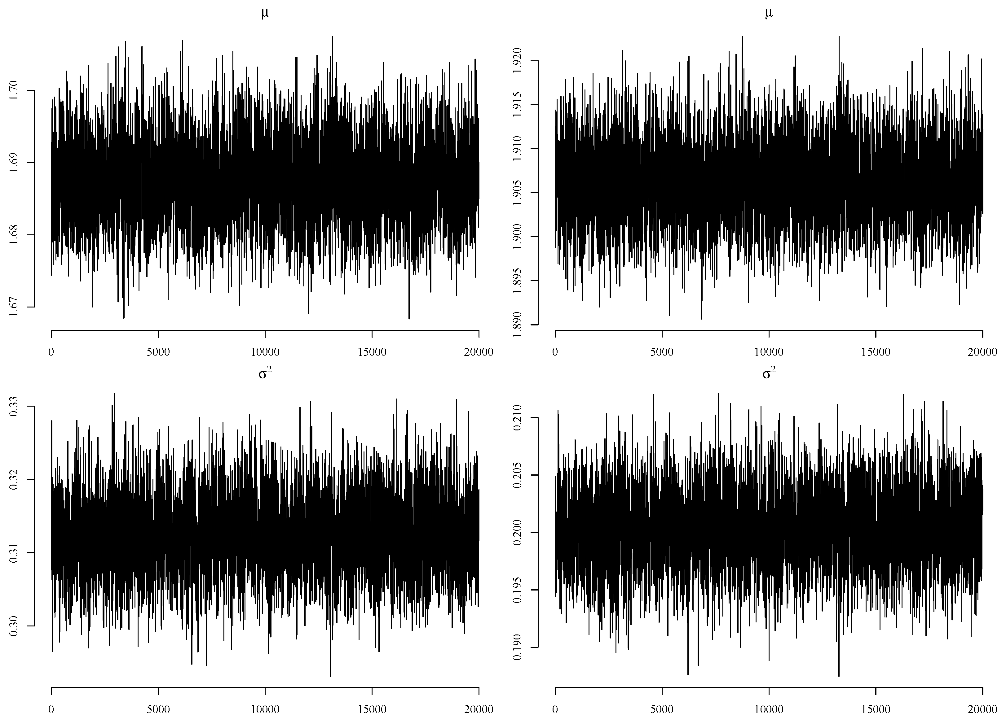
Since the LN distributions are selected from three hypothetical income distributions for both datasets, the posterior estimates from the LN distribution are shown in Table 8 with the trace plots shown in Figure 1. The trace plots confirm that the convergence of the MCMC chains is fast with respect to mixing. Therefore, we can conclude that the algorithm described in Appendix A works well for the LN distribution with the datasets. Focusing on the posterior estimates, we see that the standard deviations are very small, with narrow 95% credible intervals. This suggests that the fits of the LN distribution are very good and is the reason why the LN distributions are chosen as the hypothetical income distribution for the datasets.

Table 8. Posterior estimates of the LN distribution.

	Two-or-More Person Household					Workers’ Household
	Mean	SD	95%CI			Mean	SD	95%CI
$\mu$	1.688	0.006	1.677	1.699		1.906	0.004	1.898	1.915
${\sigma }^2$	0.313	0.005	0.303	0.323		0.200	0.003	0.194	0.207

Note: The posterior means (Mean), standard deviations (SD), and 95% credible intervals (95%CI) are displayed.

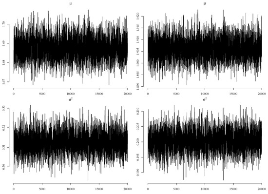
Figure 1. The trace plots for two-or-more person (left) and workers’ (right) households.

5. Conclusions

This study investigated the performance of the marginal likelihood in selecting the hypothetical income distribution from grouped data, with a specific focus on the harmonic mean estimator, using Monte Carlo simulations. The results confirmed that the harmonic mean estimator can effectively choose the appropriate hypothetical income distribution when the sample size is sufficiently large under appropriate prior settings, despite the presence of severe biases observed in the empirical example. Consequently, the harmonic mean estimator, due to its pronounced bias, may cause problems when used to compute BMA or Bayes factors, but it remains a valuable tool for selecting the appropriate model, provided the sample size is sufficient under the appropriate prior settings.

As the remaining issue, it is reasonable to examine other marginal likelihood estimators, such as those by Chan and Eisenstat (2015) and Chan (2023). It is our future remark, but our findings represent an interesting first step.

References

- Ando, T. (2010). Bayesian model selection and statistical modeling. Statistics: A Series of Textbooks and Monographs. Taylor & Francis. [Google Scholar]
- Chan, J. C. C. (2023). Comparing stochastic volatility specifications for large Bayesian VARs. Journal of Econometrics, 235(2), 1419–1446. [Google Scholar] [CrossRef]
- Chan, J. C. C., & Eisenstat, E. (2015). Marginal likelihood estimation with the cross-entropy method. Econometric Reviews, 34(3), 256–285. [Google Scholar] [CrossRef]
- Chan, J. C. C., & Grant, A. L. (2015). Pitfalls of estimating the marginal likelihood using modified harmonic mean. Economics Letters, 131, 29–33. [Google Scholar] [CrossRef]
- Chib, S. (1995). Marginal likelihood from the Gibbs output. Journal of the American Statistical Association, 90(432), 1313–1321. [Google Scholar] [CrossRef]
- Chib, S., & Jeliazkov, I. (2001). Marginal likelihood from the Metropolis–Hastings output. Journal of the American Statistical Association, 96(453), 270–281. [Google Scholar] [CrossRef]
- Chotikapanich, D., & Griffiths, W. E. (2000). Posterior distributions for the Gini coefficient using grouped data. Australian & New Zealand Journal of Statistics, 42(4), 383–392. [Google Scholar]
- Dagum, C. (1977). A new model of personal income distribution: Specification and estimation. Economie Appliquée, 30, 413–437. [Google Scholar] [CrossRef]
- Doğan, O. (2023). Modified harmonic mean method for spatial autoregressive models. Economics Letters, 223, 110978. [Google Scholar] [CrossRef]
- Doornik, J. A. (2013). OxTM 7: An object-oriented matrix programming language. Timberlake Consultants Press. [Google Scholar]
- Eckernkemper, T., & Gribisch, B. (2021). Classical and Bayesian inference for income distributions using grouped data. Oxford Bulletin of Economics and Statistics, 83(1), 32–65. [Google Scholar] [CrossRef]
- Friel, N., & Wyse, J. (2012). Estimating the evidence—A review. Statistica Neerlandica, 66(3), 288–308. [Google Scholar] [CrossRef]
- Gelfand, A. E., & Dey, D. K. (1994). Bayesian model choice: Asymptotics and exact calculations. Journal of the Royal Statistical Society. Series B (Methodological), 56(3), 501–514. [Google Scholar] [CrossRef]
- Geweke, J. (1999). Using simulation methods for Bayesian econometric models: Inference, development, and communication. Econometric Reviews, 18(1), 1–73. [Google Scholar] [CrossRef]
- Goffe, W. L., Ferrier, G. D., & Rogers, J. (1994). Global optimization of statistical functions with simulated annealing. Journal of Econometrics, 60(1–2), 65–99. [Google Scholar] [CrossRef]
- Griffiths, W. E., Chotikapanich, D., & Rao, D. S. P. (2005). Averaging income distributions. Bulletin of Economic Research, 57(4), 347–367. [Google Scholar] [CrossRef]
- Han, C., & Carlin, B. P. (2001). Markov chain Monte Carlo methods for computing Bayes factor: A comparative review. Journal of the Statistical Association, 96(455), 1122–1132. [Google Scholar] [CrossRef]
- Heyde, C. C. (1964). On a property of the lognormal distribution. Journal of the Royal Statistical Society. Series B (Methodological), 25(2), 392–393. [Google Scholar] [CrossRef]
- Heyde, C. C. (1986). Random sum distributions. In N. L. Johnson, & S. Kotz (Eds.), Encyclopedia of statistical sciences (Vol. 7, pp. 565–567). Wiley. [Google Scholar]
- Higbee, J. D., & McDonald, J. B. (2024). A comparison of the GB2 and skewed generalized log-t distributions with an application in finance. Journal of Econometrics, 240(2), 105064. [Google Scholar] [CrossRef]
- Holloway, G., Shankar, B., & Rahmanb, S. (2002). Bayesian spatial probit estimation: A primer and an application to HYV rice adoption. Agricultural Economics, 27(3), 383–402. [Google Scholar] [CrossRef]
- Kakamu, K. (2016). Simulation studies comparing Dagum and Singh-Maddala income distributions. Computational Economics, 48, 593–605. [Google Scholar] [CrossRef]
- Kakamu, K., & Nishino, H. (2019). Bayesian estimation of beta-type distribution parameters based on grouped data. Computational Economics, 54, 625–645. [Google Scholar] [CrossRef]
- Kass, R. E., & Raftery, A. E. (1995). Bayes factors. Journal of the American Statistical Association, 90(430), 773–795. [Google Scholar] [CrossRef]
- McDonald, J. B. (1984). Some generalized functions for the size distribution of income. Econometrica, 52(3), 647–665. [Google Scholar] [CrossRef]
- Newton, M. A., & Raftery, A. E. (1994). Approximate bayesian inference with the weighted likelihood bootstrap. Journal of the Royal Statistical Society. Series B (Methodological), 56(1), 3–48. [Google Scholar] [CrossRef]
- Nishino, H., & Kakamu, K. (2011). Grouped data estimation and testing of Gini coefficients using lognormal distributions. Sankhyā: The Indian Journal of Statistics, Series B, 73(2), 193–210. [Google Scholar] [CrossRef]
- Nocedal, J., & Wright, S. (2000). Numerical optimization (2nd ed.). Springer. [Google Scholar]
- Singh, S. K., & Maddala, G. S. (1976). A function for size distribution of incomes. Econometrica, 44(5), 963–970. [Google Scholar] [CrossRef]
Disclaimer/Publisher’s Note: The statements, opinions and data contained in all publications are solely those of the individual author(s) and contributor(s) and not of MDPI and/or the editor(s). MDPI and/or the editor(s) disclaim responsibility for any injury to people or property resulting from any ideas, methods, instructions or products referred to in the content. |
© 2025 by the author. Licensee MDPI, Basel, Switzerland. This article is an open access article distributed under the terms and conditions of the Creative Commons Attribution (CC BY) license (https://creativecommons.org/licenses/by/4.0/).