May 2024 Buy-Sell Guide for Dow Jones 30 Stocks and Modified Omega Criterion

Abstract

We study recent monthly data to help long-term investors buy or sell from the 30 Dow Jones Industrial Average (DJIA) Index components. The recommendations are based on six stock-picking algorithms and their average ranks. We explain the reasons for ignoring the claim that the Sharpe ratio algorithm lacks monotonicity. Since the version of “omega” in the literature uses weights that distort the actual gain–pain ratio faced by investors, we propose new weights. We use data from 30 stocks using the past 474 months (39+ years) of monthly closing prices, ending in May 2024. Our buy-sell recommendations also use newer “pandemic-proof” out-of-sample portfolio performance comparisons from the R package ‘generalCorr’. We report twelve sets of ranks for both out-of- and in-sample versions of the six algorithms. Averaging the twelve sets yields the top and bottom k stocks. For example, $k=2$ suggests buying Visa Inc. and Johnson & Johnson while selling Coca-Cola and Procter & Gamble.

1. Introduction

Investing in the stock market is vital in directing national resources to the most productive applications. The stock-picking activity of the financial services sector annually commands billions of dollars in fees. Malkiel (2013) argues that ever-growing fees for financial services are a deadweight loss for the US economy. The misallocation of resources creates waste and other losses to the economy. This paper offers tools to reduce such losses by proposing public domain stock-picking tools using free, open-source software by R Core Team (2023).

Wall Street investment outfits use stock prices attached to stock symbols. We use pretty long price data concerning 39 years and six months, ending in May 2024. If $1 is invested in buying a stock priced at $P_t$ at time t, if the price (adjusted for dividends) at time $t+1$ is higher, the net return $r_t=[(P_{t+1}-P_t)/P_t]$ will exceed the initial investment of $1. Since the net return is negative when losses are incurred, one defines the gross return as $(1+r_t)=1+(P_{t+1}-P_t)/P_t=P_{t+1}/P_t$. The gross return is always positive since prices are positive.

Continuously compounded return is the exponential return, $exp\left(r_t\right)$, which is always positive. The series expansion of $exp\left(r_t\right)$ is $(1+r_t+r_t^2/2!+..)$. Assuming higher order terms in the expansion can be ignored, ($|r_t|<1)$, one can write exp$\left(r_t\right)=1+r_t$. It is customary to equate the exponential return to the gross return and write $r_t=log(P_{t+1}/P_t)=log{P}_{t+1}-log{P}_t$. Many published papers use the first difference of logs of prices evaluated at time $t+1$ as a return from investment. Since the return data do not always satisfy ($|r_t|<1$) for certain time periods, let us define $r_t=[(P_t-P_{t-1})/P_{t-1}]$ for our monthly returns from the Dow Jones Industrial Average’s 30 (DJ30) stocks.

Let $f\left(r\right)$ denote the probability distribution function of returns ($r)$ from investing in one of the 30 stocks, and let $F\left(r\right)$ denote the (cumulative) distribution function of returns. Denote the expected value (mean) of $f\left(r\right)$ by $\mu$ and the standard deviation by $\sigma$. The Sharpe ratio, Sharpe (1966), is named after a Nobel-winning economist. It represents a risk-adjusted average return from investment X, defined as

$$SR\left(r_X\right)=\mu \left(r_X\right)/\sigma \left(r_X\right),$$

(1)

where the denominator makes risk adjustment. Typical SR ranks investment opportunities based on data on market returns represented by the probability distribution $f\left(r\right)$ mentioned before.

Although (1) can also be used for ranking gambles, this paper uses it for stock-picking. Gambling is a zero-sum or negative-sum game. By contrast, buying (selling) a share of companies contributing to socially desirable (undesirable) goods and services often yields positive $\mu$ and a larger $SR$.

Aumann and Serrano (2008) propose an ‘index of riskiness’ of an investment as if it is a gamble. They conjure imaginary gambling situations to assess their riskiness using an axiomatic framework and an economic decision-making context. They reject the reciprocal of $SR$ of (1) as a measure of riskiness because it fails monotonicity property based on first-order stochastic dominance. Aumann and Serrano (2008) focus too much on the attributes of the stock buyer measured by a buyer’s risk-averse utility function. These authors refer to a constant absolute risk-averse “CARA person” (page 816).

Cheridito and Kromer (2013), or “CK13,” is an impressive study of mathematical formulas defining 45 performance measures similar to the reward–risk ratio (1). Among the 45 are tweaks on Sharpe ratios and ratios involving the value at risk (VaR). They evaluate the following four properties:

• (M) monotonicity means that more is better than less. This is a common-sense minimal requirement. All performance measures should satisfy it.
• (Q) Quasi-concavity describes uncertainty aversion linked to economists’ utility and decision theories. It is not relevant if we include investors who allocate a (small) proportion of investor funds as if they are risk-loving. We need not accept this criterion for our purposes.
• (S) Scale Invariance or $SR\left(X\right)=SR\left(\lambda X\right)$ where $\lambda$ is a constant. The invariance requirement is inappropriate for modern investing where some technologies need very large (or small) scale and transaction costs are low for large transactions.
• (D) Distribution-based. All six stock-picking algorithms in this paper are distribution-based.

CK13 evaluations are not necessarily for stock market investment, but include the ranking of gambles where the “probability measure” (as in the measure theory of Statistics) may be unknown. By contrast, our probability measure is well approximated by $f\left(r\right)$, and its riskiness is well represented by its dispersion. CK13 claim that 17 measures out of 45, including the Sharpe ratio (SR), fail to meet the minimal monotonicity requirement (M). The next four paragraphs show the limitations of the CK13 claim. We shall show that CK13 proof assumes certain artificial gambles that are irrelevant for our stock-picking based on $f\left(r\right)$.

Proposition 4.1 in CK13 allegedly proves that $SR=\mu \left(X\right)/\sigma \left(X\right)$ fails (M). The proof involves the existence of pathological cases involving three constants satisfying properties as follows: [$(a,b,c)>0,a>c,b\ge 1,bc>a$]. The proof needs to assume a non-negative random variable $Z\ge 0$. Since stock returns can be both positive and negative, the assumption $Z\ge 0$ is invalid for our $f\left(r\right)$.

We begin by showing that SR fails (M) when $Z\ge 0$. CK13 proof defines $X=a+b\ast Z$ and $Y=c+Z$. For example, choose $a=2.5,b=2.4,c=1.5,Z=1$, and $\sigma \left(Z\right)=1$. Now, $X=2.5+2.4\ast Z=4.9$ and $Y=1.5+Z=2.5$, with $X>Y$. Now, $E\left(X\right)=4.9$ is 96% larger than $E\left(Y\right)=2.5$, whereas $\sigma$(X) = 2.4 is 240% larger than $\sigma$(Y) = 1. Hence, $SR\left(X\right)=4.9/2.4=2.04<SR\left(Y\right)=2.5$. Since X is larger while $SR\left(X\right)$ is smaller, the Sharpe ratio indeed fails (M) for $Z\ge 0$.

Consider a realistic negative realization of the random variable Z, representing losses, with $Z=-1$. Let us keep the above choices of $(a,b,c)$ and formulas for X and Y in CK13 unchanged. Now, $X=2.5+2.4\ast Z=0.1$ and $Y=1.5+Z=0.5$, implying that $X<Y$. This $E\left(X\right)=0.1$ is 500% smaller than $E\left(Y\right)=0.5$, whereas $\sigma$(X) = 2.4 is 240% larger than $\sigma$(Y) = 1. Hence, $SR\left(X\right)=0.1/2.4=0.04<SR\left(Y\right)=2.5$. Since X is smaller while $SR\left(X\right)$ is also smaller, the Sharpe ratio passes (M).

The CK13 alleged failure to pass (M) holds only for artificially constructed gambles satisfying peculiarly demanding unrealistic restrictions $(X=a-bc+bY)$ with a non-negative random variable Z denying any presence of losses, unlike typical $f\left(r\right)$. Thus, stock market investors can safely ignore the claim that SR fails (M).

We further argue that property (Q) linked to utility theory can be ignored when allocating resources. After all, economists have long avoided interpersonal utility comparisons. An individual investor’s utility experience is personal, rarely identical across individuals, and exhibits marked change for the same individual over time and space. Psychologists have documented that utility from profits and losses is asymmetric and sensitive to profit and loss sizes. It is futile to assess whether someone is a “CARA person” before deciding which decision theory applies to him. In summary, the M, Q, S, and D criteria proposed by CK13 can be misleading when applied to stock-picking purposes.

Let us turn to the 30 stocks comprising DJIA. We begin with Table 1 and Table 2 for the company names studied here in two parts with fifteen companies each. We report ticker symbols, relative weights in DJIA, and a (case-sensitive) single-character name to identify the stock for later use in graphics and tables. Figure 1 is inspired by Markowitz’s efficient frontier model, without the straight line representing a risk-free rate. This Figure has the mean return on the vertical axis and the standard deviation of returns measuring the volatility (risk) for that stock on the horizontal axis. We depict thirty letters in Figure 1 for each DJIA index component sticker.

Table 1. Company names, ticker symbols, weight in DJIA, and abbreviations with only one character. Part 1.

Seq.	Company	Symbol	Weight	Char1
1	Apple Inc.	AAPL	2.93	a
2	Amgen Inc.	AMGN	4.65	A
3	Amazon.com Inc.	AMZN	2.99	z
4	American Express Co.	AXP	4.09	x
5	Boeing Co.	BA	2.88	b
6	Caterpillar Inc.	CAT	5.83	c
7	Salesforce Inc.	CRM	4.71	C
8	Cisco Systems Inc.	CSCO	0.83	S
9	Chevron Corp.	CVX	2.85	e
10	Walt Disney Co.	DIS	1.94	d
11	Dow Inc.	DOW	0.97	D
12	Goldman Sachs Group Inc.	GS	7.24	g
13	Home Depot Inc.	HD	5.72	h
14	Honeywell International Inc.	HON	3.33	H
15	Intl Business Machines Corp.	IBM	2.91	i

Table 2. Company names, ticker symbols, weight in DJIA, and abbreviations with only one character. Part 2.

Seq.	Company	Symbol	Weight	Char1
16	Intel Corp.	INTC	0.61	I
17	Johnson & Johnson	JNJ	2.53	j
18	JP Morgan Chase & Co.	JPM	3.33	J
19	Coca Cola Co.	KO	1.06	k
20	McDonald’s Corp.	MCD	4.75	m
21	3m Co.	MMM	1.58	M
22	Merck & Co. Inc.	MRK	2.25	K
23	Microsoft Corp.	MSFT	6.88	f
24	Nike Inc Cl B	NKE	1.62	n
25	Procter & Gamble Co.	PG	2.80	p
26	Travelers Cos Inc.	TRV	3.69	t
27	Unitedhealth Group Inc.	UNH	8.52	u
28	Visa Inc Class A Shares	V	4.75	v
29	Verizon Communications Inc.	VZ	0.68	V
30	Walmart Inc.	WMT	1.04	w

Figure 1. Mean–standard deviation efficiency frontier for Dow Jones 30 stocks.

The basic idea behind Figure 1 is that we imagine grouping stocks into a certain number (=7) of unequal width ranges of standard deviation class intervals. Our 30 stocks are implicitly assigned to these seven $\sigma$ intervals. Now, the stock yielding the highest average return for each level of risk (measured by the midpoints of the sd class interval) dominates all those below it in Figure 1. The dominating stocks from DJIA are graphically identified as (j, v, h, f, C, a, z). The corresponding longer company names of dominating stocks, according to Table 1 and Table 2, are Johnson & Johnson, Visa, Home Depot, Microsoft, Salesforce, Apple, and Amazon.

1.1. Descriptive Statistics for the DJIA Stock Returns

This section reports some basic information about our data using standard descriptive stats. We report ‘min’ for the smallest return, Q1 for the first quartile, where 25% of data are below Q1 and 75% are above Q1. ‘Median’ and ‘Mean’ are self-explanatory. Q3 is for the third quartile (75% below and 25% above), and ‘max’ denotes the largest return.

In finance, two additional descriptive stats are referenced. The $SR=\mu /\sigma$ defined before and the ‘expected gain–expected pain ratio’. The latter is called ‘omega’ ($\Omega$) in Keating and Shadwick (2002), or “KS02” hereafter. While we include $SR$ and $\Omega$ among the descriptive statistics associated with each stock, we include them among our six stock-picking algorithms.

1.1.1. Sharpe Ratios for Risk-Adjusted Stock Returns

The $SR$ of (1) is a popular stock-picking tool. Many researchers have studied it and suggested modifications. $SR$ treats a symmetric measure $\sigma$ as an approximation to the risk. It treats volatility on the profit and loss side as equally undesirable. Volatility on the loss side is undesirable but desirable on the profit side. An adjusted version, $S{R}_{dsd}=\mu /DSD$, replaces the $\sigma$ in the original denominator by downside standard deviation ($DSD=\surd DSV$) from the square root of DSV, the downside variance. Let $n^b$ denote the number of observations below the mean. The downside variance in Vinod and Reagle (2005) (page 111, Equation (5.2.2)) is computed as

$$DSV=\left[{\Sigma }_t{w}_t{(r_t-\overline{r})}^2\right]/n^b,$$

(2)

where $w_t=0$ when $r_t>\overline{r}$, and $w_t=1$ otherwise. The summation is over $n^b$ returns involving possible losses. The adjusted version

$$S{R}_{dsd}=\mu /\surd DSV,$$

(3)

is not difficult to compute. The online Appendix A provides software for $S{R}_{dsd}$.

Page 114 of Vinod and Reagle (2005) was perhaps the first to identify an often-ignored serious problem with Sharpe ratios. Now, we show how SR provides the wrong rankings when risk-adjusting any stocks with negative average returns. We explain the wrong ranking using an example of two stocks, p and q, with Sharpe ratios, $S{R}_p={\mu }_p/{\sigma }_p$, and $S{R}_q={\mu }_q/{\sigma }_q$. Now, assume that both have a negative average loss of 100, or ${\mu }_p={\mu }_q=-100$. Next, assume that stock p is twice as volatile (risky) as stock q, or ${\sigma }_p=10$ and ${\sigma }_q=5$. We expect that the money-losing and more risky stock p is worse than q. Note that $S{R}_p=-100/10=-10$ is larger than $S{R}_q=-100/5=-20$. The ranking by $SR$ says q is worse than p, which is against common sense.

Page 114 of Vinod and Reagle (2005) also explains how to use suitably large “add factors” to obtain the $SR$ to yield the correct ranking. Fortunately, columns entitled ‘Mean’ in Table 3 and Table 4 (of descriptive stats reported later) show that all thirty stocks have positive average returns. Thus, we do not need any ‘add factor’ adjustment in our context.

Note that our $SR=\mu /\sigma$ assumes that the researcher has true unknown values of $\mu$ and $\sigma$, rather than their sample estimates ignoring estimation errors. A “Double Sharpe ratio” divides the sample estimate $\widehat{sr}$ by its standard error (SE), the standard deviation of the sampling distribution. The division penalizes stocks with a higher estimation risk. A double SR, which penalizes for estimation risk represented by a bootstrap standard error, is discussed on page 227 of Vinod and Reagle (2005). We denote it as SR with subscript ‘se’ as

$$S{R}_{se}=\widehat{sr}/SE\left(sr\right),$$

(4)

The online Appendix A provides software for computing $S{R}_{dsd}$ of (3) using downside standard deviation in the denominator. Next, the appendix software computes a large number J of $S{R}_{dsd}^j$ based on bootstrap replicates. Then, the code computes $SE\left(sr\right)$ in the denominator of (4), which becomes the standard deviation of J bootstrap values $S{R}_{dsd}^j$.

Recall that the risk (horizontal axis) versus return (vertical axis) scatterplot of Figure 1 suggests that Johnson & Johnson, Visa, Home Depot, Microsoft, Salesforce, Apple, and Amazon graphically dominate others. The respective Sharpe ratios of these stocks are (0.22, 0.26, 0.23, 0.25, 0.22, 0.19, 0.15). Note that the Sharpe ratio is a direct measure of risk-adjusted return, bypassing the grouping of stock returns into standard deviation (sd) intervals.

The lowercase versions of ticker symbols for the top seven Sharpe ratios in increasing order of magnitude are amzn = 0.22, jnj = 0.22, crm = 0.22, unh = 0.23, hd = 0.23, msft = 0.25, and v = 0.26, respectively. Markowitz’s theory supports a stock-picking algorithm based on the Sharpe ratio. It is one of the six algorithms listed later in Section 3.

1.1.2. Original Computation of “Omega” for Stock Returns

KS02 name a “cumulative probability weighted” gain–loss ratio “omega” ($\Omega$), and claim that it is a “universal” performance measure. We regard it as one of many and find that the weighting used in its original computation can be simplified without sacrificing its intent. This subsection describes the need for simplification, while the following subsection describes a recommended version. A referee has suggested that some readers are not interested in knowing exactly how our simplified version maintains the intent behind the gain–loss ratio. Uninterested readers can skip the present subsection.

The title of KS02 claims universality for their performance measure. Since a larger omega means a larger preponderance of positive returns, a stock having a larger omega is more desirable. The idea of measuring a gain–loss ratio is first mentioned by Bernardo and Ledoit (2000), who define r as a risk-adjusted excess return over a target return. Their risk adjustment requires assumptions about the utility function of investors. This paper avoids any assumption regarding investor utility functions. We retain their distinction between $r^{+}=max(0,r)$, the positive part of returns, and $r^{-}=max(r,0)$, the negative part. Their gain–loss ratio is ${\Omega }_{bl}$, (where the subscript ‘bl’ identifies authors) is as follows:

$${\Omega }_{bl}=E\left(r^{+}\right)/E\left(r^{-}\right).$$

(5)

Section 3.1 of CK13 states that Bernardo–Ledoit-type ratios satisfy all four (M, Q, S, D) properties mentioned above.

KS02 do not assume anything about the utility function of investors. The gains and losses in KS02 are compared to a target return. If all stocks in a data set have a common target return, we can subtract it from all returns and work with returns in “excess of target”. Hence, there is no loss of generality in letting the target be zero. Therefore, our target return is mostly zero in the sequel. Metel et al. (2017) explain how omega generalizes the mean variance-based Sharpe ratio by encompassing the entire $f\left(r\right)$ (page 4) “therefore incorporating higher moment properties”. Their Theorem 1 proves that, within the class of elliptical density functions, using the Sharpe ratio or the Omega measure to optimize portfolio performance leads to the same optimal portfolio. The theorem has no practical implications for our purposes when working with real-world market returns, usually not from any known density.

KS02 define

$${\Omega }_{ks}=E\left(gain\right)/E\left(loss\right),$$

(6)

where the expectation operator from the probability theory in $E\left(gain\right)$ is represented by choosing weights ($1-F\left(r\right)$) by assuming continuous distributions. Similarly, KS02 represent $E\left(loss\right)$ by choosing $F\left(r\right)$ weights. The subscript ‘ks’ in ${\Omega }_{ks}$ identifies the authors of KS02.

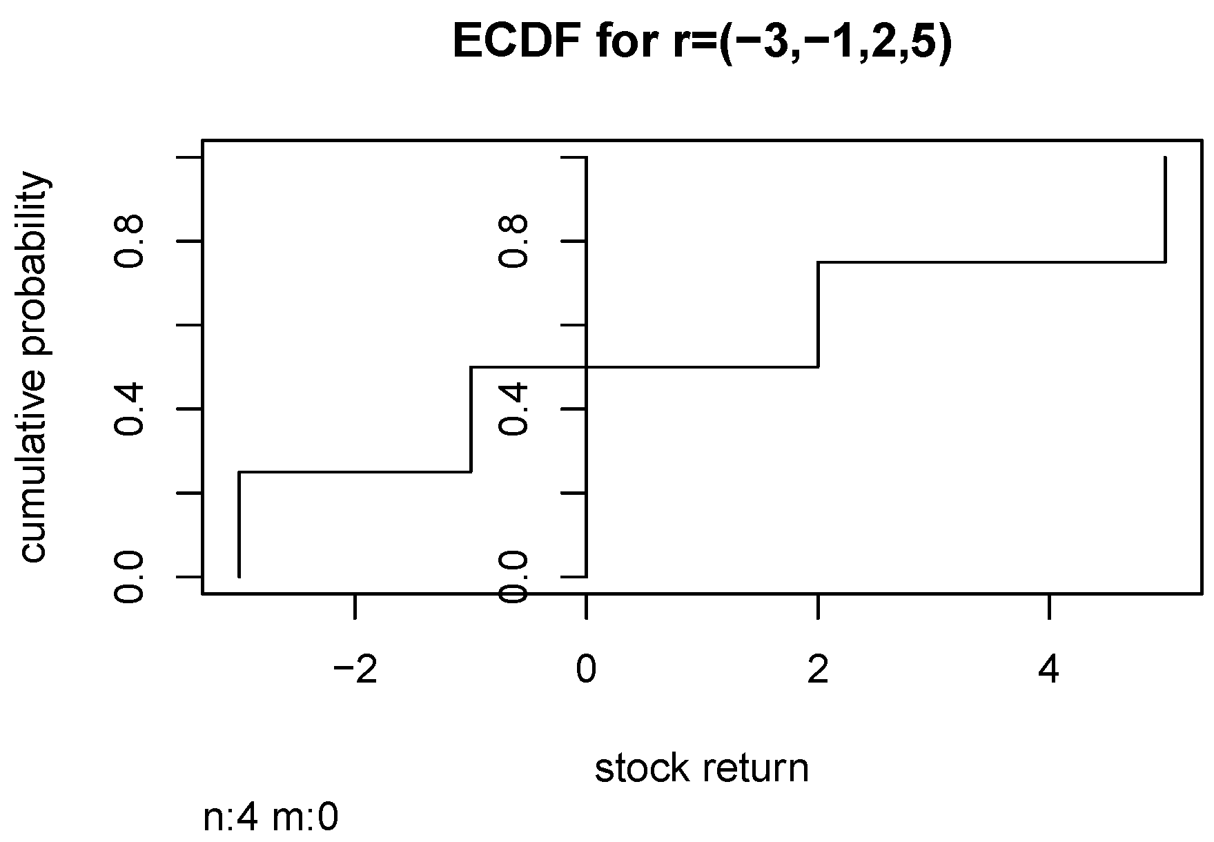
Considerable literature on “omega” assumes a continuous $f\left(r\right)$, usually with a known (Gaussian, Elliptical) form. By contrast, this paper assumes a nonparametric representation of $f\left(r\right)$ based on actual market returns data. Since observable data are always discrete, we replace $F\left(r\right)$ with the empirical cumulative distribution function (ECDF), a step function of returns. It uses all the information in the data on returns and is considered a “sufficient statistic”.

Figure 2 illustrates the ECDF for an imaginary stock A with $n=4$, returns $r_t=(-3,-1,2,5)$, for $t=1,2,.,n.$ A vertical axis at $r=0$, shown in Figure 2, separates the ECDF for stock A into the loss side on the left (for $r^{-}=max(r,0)$) and the gain side on the right (for $r^{+}=max(0,r)$).

Figure 2. Empirical Cumulative Distribution Function for a Toy Example.

How do we represent the E operator weights in the discrete case? Usually, mathematical expectation $E\left(x\right)=\Sigma x_t{p}_t$ (return $x_t$ with probability $p_t$) is the average return. KS02 formulate the mathematical expectation of aggregate loss based on cumulative sums of negative returns $r_t$ times corresponding cumulative probabilities from $F\left(r\right)$ as weights. Their gain side weights based on ($1-F\left(r\right)$) are from the areas above the ECDF steps. The following paragraph uses Figure 2 to explain the numerical computation of KS02’s cumbersome weighting for toy stock A mentioned above.

The ECDF on the loss side for toy stock A has two negative ranges, (box intervals) ($-3,-1$) and ($-1,0$), with areas under the pillars for the two ranges of (1/n) and (2/n), respectively. The respective gain side weights (2/n) and (1/n) are based on ($1-F\left(r\right)$). These weights represent the areas above the pillars for the two ECDF ranges (0, 2) and (2, 5) on the right-hand side of the zero axis in Figure 2.

The KS02 weighting scheme of ${\Omega }_{ks}$ appears to be the same as that of the partial moments of degree 1. Hence, ${\Omega }_{ks}$ of (6) is the ratio of the upper partial moment (UPM) of degree 1 to the analogous lower partial moment (LPM), Viole and Nawrocki (2016). In the R package called NNS, Viole (2021) has convenient functions called UPM and LPM to compute them, and hence

$${\Omega }_{ks}=UPM(1,0,r)/LPM(1,0,r),$$

(7)

where r is a vector of returns, and where we have included the arguments (degree = 1, target = 0) of the R functions in the NNS package. Considering that these ratios are decades old, there is a need to compare the out-of-sample performance of ${\Omega }_{ks}$ from stock market return data using the NNS package with the three versions of Sharpe ratios in Equations (1), (3), and (4).

This subsection has explained the logic behind the cumbersome weighting scheme in KS02. The following subsection shows how the ECDF weighting is not really needed to achieve the intent in Bernardo and Ledoit (2000).

1.1.3. Recommended Computation of “Omega” for Stock Returns

Recall that we regard omega as one of many stock-picking algorithms. This subsection suggests a direct computation of Equation (5) for aggregate gain–aggregate loss ratios without using $F\left(r\right)$ and $(1-F(r\left)\right)$ weights. We divide the vector of returns $r_t$ into positive $\left(r_t^{+}\right)$ and negative $\left(r_t^{-}\right)$ parts, proposing

$${\Omega }_{sum}={\displaystyle \frac{{\Sigma }_t\left(r_t^{+}\right)}{{\Sigma }_t\left|\left(r_t^{-}\right)\right|}},$$

(8)

where the subscript ‘sum’ refers to summations in the formula. The numerator and denominator are both positive. For example, the stock A with returns $r_t^A=(-3,-1,2,5)$ has ${\Omega }_{sum}=((2+5)/(3+1))=7/4$. The stock B with returns $r_t^B=(-4,1,2,4)$ has the same ${\Omega }_{sum}=7/4$. The computation of ${\Omega }_{sum}$ is seen to be easy and intuitive.

An alternative formulation is

$${\Omega }_{avg}={\displaystyle \frac{{\Sigma }_t\left(r_t^{+}\right)/n^{+}}{{\Sigma }_t\left|\left(r_t^{-}\right)\right|/n^{-}}},$$

(9)

where $n^{+}$ denotes the number of positive returns in the data, $n^{-}$ denotes the number of negative returns, and the subscript ‘avg’ refers to the averages in the formula. If the stock returns arose from an independent and identically distributed (IID) process, the probability of observing each return $r_t$ is 1/n and averages equal mathematical expectations. Hence, it is tempting to prefer ${\Omega }_{avg}$ over ${\Omega }_{sum}$. However, market returns are almost never IID. A stock’s return is intimately related to its own past, the returns of other stocks in its class, the socio-political conditions, etc. Since the joint density of all stocks is unknown, the probability of the sum of k returns (${\Sigma }^k{r}_t)$ is also unknown.

Can we use the averages in ${\Omega }_{avg}$ as an approximation by pretending that returns are IID? Let us compare the two formulas (8) and (9). Observe that ${\Omega }_{avg}$ is larger than ${\Omega }_{sum}$ when $n^{-}$ is large, and that ${\Omega }_{avg}$ is smaller when $n^{+}$ is large. The total gain–loss ratio is being multiplied by ($n^{-}/n^{+}$). What are the implications of the relative sizes of ($n^{+},n^{-}$) to the investor’s bottom line? We use two imaginary stocks, A and B, to argue that a larger (smaller) ratio ($n^{-}/n^{+}$) does not benefit (hurt) the bottom line of the investor and should be ignored.

Assume two sets of stock returns $r_t^A=(-3,-1,2,5)$ and $r_t^B=(-4,1,2,4)$. They have the same ${\Omega }_{sum}^A=1.75={\Omega }_{sum}^B$, though the $1.75={\Omega }_{avg}^A>>{\Omega }_{avg}^B=7/12=0.58333$. If one relies on ${\Omega }_{avg}^B$, we have to conclude that the gain–pain ratio for stock A is over three times better than stock B. The aggregate gain (=7), aggregate loss (=4), and gain–loss ratio (7/4 = 1.75) to the investor is exactly the same for stocks A and B. The aggregate gain of 7 for stock B is spread over $n_B^{+}=3$ periods, while the aggregate loss (=4) is spread over only one period $n_B^{-}=1$. The aggregate gain and loss for stock A is spread over two periods $n_A^{+}=2=n_A^{-}$. The practically irrelevant (to the investor) sizes of ($n^{+},n^{-}$) should not be allowed to contaminate the computation of the gain–loss ratio. We conclude this section by stating that there are sound reasons for rejecting ${\Omega }_{avg}$ of (9) in favor of the simpler ${\Omega }_{sum}$ of (8).

Table 3. Table of basic descriptive stats. ‘Sharpe’ is the ratio of mean to standard deviation (sd). ${\Omega }_s$ is ${\Omega }_{sum}$, the sum of all positive returns divided by the sum of all negative returns. Number of non-missing or available sample size in the last column, ‘Av.N’. Part 1.

Ticker	Min	Q1	Median	Mean	Q3	Max	Sd	Sharpe	${\mathbf{\Omega }}_{\mathit{s}}$	Av.N
aapl	−57.74	−4.66	2.53	2.40	9.81	45.38	12.20	0.20	1.7	473
amgn	−41.53	−3.62	1.59	2.17	6.36	45.88	9.94	0.22	1.9	473
amzn	−41.16	−4.73	2.47	3.61	9.74	126.38	16.56	0.22	2.0	324
axp	−32.09	−2.38	1.37	1.31	5.86	85.03	8.72	0.15	1.6	473
ba	−45.47	−3.82	1.45	1.18	6.99	45.93	8.83	0.13	1.4	473
cat	−35.91	−4.16	1.69	1.52	7.15	40.14	8.96	0.17	1.6	473
crm	−36.03	−4.61	1.75	2.39	8.98	40.26	11.08	0.22	1.8	239
csco	−36.73	−4.01	1.70	2.19	8.27	38.92	10.48	0.21	1.8	411
cvx	−21.46	−2.57	1.09	1.15	4.76	26.97	6.47	0.18	1.6	473
dis	−28.64	−3.34	1.05	1.28	5.73	31.26	7.91	0.16	1.5	473
dow	−26.45	−3.37	1.24	0.86	6.30	25.48	9.41	0.09	1.3	62
gs	−27.73	−5.20	1.33	1.15	6.64	31.38	9.22	0.12	1.4	300
hd	−28.57	−3.41	1.71	1.91	7.06	30.33	8.14	0.23	1.8	473
hon	−38.19	−2.39	1.33	1.18	5.06	51.05	7.75	0.15	1.5	473
ibm	−24.86	−3.61	0.75	0.84	5.00	35.38	7.44	0.11	1.4	473

Table 3. Table of basic descriptive stats. ‘Sharpe’ is the ratio of mean to standard deviation (sd). ${\Omega }_s$ is ${\Omega }_{sum}$, the sum of all positive returns divided by the sum of all negative returns. Number of non-missing or available sample size in the last column, ‘Av.N’. Part 1.

Ticker	Min	Q1	Median	Mean	Q3	Max	Sd	Sharpe	${\mathbf{\Omega }}_{\mathit{s}}$	Av.N
aapl	−57.74	−4.66	2.53	2.40	9.81	45.38	12.20	0.20	1.7	473
amgn	−41.53	−3.62	1.59	2.17	6.36	45.88	9.94	0.22	1.9	473
amzn	−41.16	−4.73	2.47	3.61	9.74	126.38	16.56	0.22	2.0	324
axp	−32.09	−2.38	1.37	1.31	5.86	85.03	8.72	0.15	1.6	473
ba	−45.47	−3.82	1.45	1.18	6.99	45.93	8.83	0.13	1.4	473
cat	−35.91	−4.16	1.69	1.52	7.15	40.14	8.96	0.17	1.6	473
crm	−36.03	−4.61	1.75	2.39	8.98	40.26	11.08	0.22	1.8	239
csco	−36.73	−4.01	1.70	2.19	8.27	38.92	10.48	0.21	1.8	411
cvx	−21.46	−2.57	1.09	1.15	4.76	26.97	6.47	0.18	1.6	473
dis	−28.64	−3.34	1.05	1.28	5.73	31.26	7.91	0.16	1.5	473
dow	−26.45	−3.37	1.24	0.86	6.30	25.48	9.41	0.09	1.3	62
gs	−27.73	−5.20	1.33	1.15	6.64	31.38	9.22	0.12	1.4	300
hd	−28.57	−3.41	1.71	1.91	7.06	30.33	8.14	0.23	1.8	473
hon	−38.19	−2.39	1.33	1.18	5.06	51.05	7.75	0.15	1.5	473
ibm	−24.86	−3.61	0.75	0.84	5.00	35.38	7.44	0.11	1.4	473

Table 4. Table of basic descriptive stats. Sharpe is the ratio of mean to standard deviation (sd). ${\Omega }_s$ is ${\Omega }_{sum}$, the sum of all positive returns divided by the sum of all negative returns. Number of non-missing or available sample size in the last column, ‘Av.N’. Part 2.

Ticker	Min	Q1	Median	Mean	Q3	Max	Sd	Sharpe	${\mathbf{\Omega }}_{\mathit{s}}$	Av.N
intc	−44.47	−4.39	1.25	1.52	7.05	48.81	10.67	0.14	1.5	473
jnj	−16.34	−2.23	1.25	1.22	4.43	19.29	5.59	0.22	1.8	473
jpm	−32.68	−3.86	1.22	1.32	6.36	33.75	9.17	0.14	1.5	473
ko	−19.33	−2.08	1.24	1.20	4.62	22.64	5.83	0.21	1.7	473
mcd	−25.67	−2.16	1.36	1.26	5.04	18.26	5.94	0.21	1.7	473
mmm	−27.83	−2.46	1.22	1.01	4.40	25.80	6.07	0.17	1.5	473
mrk	−26.62	−3.02	1.12	1.33	5.86	23.29	6.94	0.19	1.6	473
msft	−34.35	−3.56	2.25	2.36	6.80	51.55	9.45	0.25	2.0	458
nke	−37.50	−3.30	1.84	1.90	7.02	39.34	9.40	0.20	1.7	473
pg	−35.42	−1.77	1.20	1.20	4.92	24.69	5.57	0.22	1.8	473
trv	−53.47	−3.17	1.42	1.09	5.03	52.51	7.34	0.15	1.5	473
unh	−36.51	−3.21	2.50	2.18	7.39	40.70	9.57	0.23	1.9	473
v	−19.69	−2.47	2.27	1.58	5.25	16.83	6.14	0.26	1.9	194
vz	−20.48	−2.75	0.52	0.89	4.92	37.61	6.17	0.14	1.5	473
wmt	−27.06	−2.40	1.25	1.37	5.55	26.59	6.48	0.21	1.7	473

Table 4. Table of basic descriptive stats. Sharpe is the ratio of mean to standard deviation (sd). ${\Omega }_s$ is ${\Omega }_{sum}$, the sum of all positive returns divided by the sum of all negative returns. Number of non-missing or available sample size in the last column, ‘Av.N’. Part 2.

Ticker	Min	Q1	Median	Mean	Q3	Max	Sd	Sharpe	${\mathbf{\Omega }}_{\mathit{s}}$	Av.N
intc	−44.47	−4.39	1.25	1.52	7.05	48.81	10.67	0.14	1.5	473
jnj	−16.34	−2.23	1.25	1.22	4.43	19.29	5.59	0.22	1.8	473
jpm	−32.68	−3.86	1.22	1.32	6.36	33.75	9.17	0.14	1.5	473
ko	−19.33	−2.08	1.24	1.20	4.62	22.64	5.83	0.21	1.7	473
mcd	−25.67	−2.16	1.36	1.26	5.04	18.26	5.94	0.21	1.7	473
mmm	−27.83	−2.46	1.22	1.01	4.40	25.80	6.07	0.17	1.5	473
mrk	−26.62	−3.02	1.12	1.33	5.86	23.29	6.94	0.19	1.6	473
msft	−34.35	−3.56	2.25	2.36	6.80	51.55	9.45	0.25	2.0	458
nke	−37.50	−3.30	1.84	1.90	7.02	39.34	9.40	0.20	1.7	473
pg	−35.42	−1.77	1.20	1.20	4.92	24.69	5.57	0.22	1.8	473
trv	−53.47	−3.17	1.42	1.09	5.03	52.51	7.34	0.15	1.5	473
unh	−36.51	−3.21	2.50	2.18	7.39	40.70	9.57	0.23	1.9	473
v	−19.69	−2.47	2.27	1.58	5.25	16.83	6.14	0.26	1.9	194
vz	−20.48	−2.75	0.52	0.89	4.92	37.61	6.17	0.14	1.5	473
wmt	−27.06	−2.40	1.25	1.37	5.55	26.59	6.48	0.21	1.7	473

2. Unbiased Out-of-Sample Calculations

Most authors define their out-of-sample range from the last few periods of the data. Since any such out-of-sample time series is sensitive to the peculiar characteristics of the last few periods, their calculations can be biased. For example, if the out-of-sample (oos) series coincides with the 2020 pandemic, the calculations will have a pessimistic bias. Vinod (2023) suggests removing the bias by “pandemic proofing” the calculations on (40% here) randomly chosen ‘oos’ data. Each j-th choice yields a ranking of stocks. Repeating the ranking J (=50, say) times, we compute their mean $\mu$ and standard deviation $\sigma$ for the i-th stock-picking algorithm. We have $i=1,\dots ,6$ here. Assuming no transaction costs, Vinod (2023) computes a zero-cost arbitrage, executing the following trades. One short sells (selling without first possessing) certain dollars worth of the worst stock in DJIA and buys the appropriate fraction of the best stock as determined by each method.

Our unbiased ‘oos’ strategy here does not seek a zero-cost arbitrage. Instead, we just compute distinct stock rankings by each method in-sample and randomly choose 40% observations for each j-th ‘oos’ realization. Finally, the average of the ranks over $j=1,\dots ,J$ random choices determines the ‘oos’ stock choice by that method.

3. Ranking 30 Stocks by Six Algorithms

We split our report into three tables, ranking the 30 DJIA stocks by two versions of six stock-picking algorithms. Each table has ten stocks at a time in alphabetical order of their ticker symbols. Table 5, Table 6 and Table 7 report two versions of the ranks produced by each algorithm for (a) in-sample ranks and (b) unbiased out-of-sample ranks.

• Sharpe-in/out: Section 1.1.1 mentions the Sharpe ratio as a stock-picking algorithm.
• Omega-in/out: Our computation is described in Section 1.1.3 and Equation (8) for ${\Omega }_{sum}$.
• Decile-in/out: It is generally agreed that the stock whose probability distribution of returns is more to the right-hand side is more desirable. One way to achieve this is to compare their deciles. The R package ‘generalCorr,’ offers a convenient function called decileVote(.).
• Descr-in/out: We compare the traditional descriptive stats of each stock’s data. Most stats are in the “the larger, the better” category and are obtains (+1) as weight. The standard deviation represents risk and obtains (−1) weight. This algorithm uses a weighted summary of these stats for stock-picking.
• Momen-in/out: Moment values: The first four moments of a probability distribution provide information about centering, variability, skewness, and kurtosis. Our weights incorporate the prior knowledge that low variability and low kurtosis are desirable, while larger mean and skewness are desirable. A weighted summary is implemented in the R package ‘generalCorr,’ function called momentVote(.).
• Exact-in/out: This algorithm refers to the exact stochastic dominance mentioned in Section 3.1. The stochastic dominance (SD) of the first four orders is summarized in the R package ‘generalCorr’. See the R function called exactSd(). The theoretical details are available in Vinod (2024), where iterated integrals of cumulative distribution functions are used. See the following Section 3.1 for a summary of general ideas behind the theory of stochastic dominance.

3.1. Ranking Stocks by Exact Stochastic Dominance

We apply some of the tools described in Vinod (2024) to the portfolio selection problem for the DJ30 data set used here. We use the exact computation of stochastic dominance using a worse imaginary stock (x.ref) than the worst-performing stock in DJ30.

We shall see that stochastic dominance needs a reference stock. Accordingly, we plan to compute the return for each of the 30 DJIA stocks with reference to the return in excess of the money-losing imaginary 31-st stock (x.ref). The lowest return over all included DJ30 data sets and over all 30 stocks is $-86.14151$, where the negative sign suggests a loss. Let us choose (x.ref) return $-87.38904$, which is a little smaller than $-86.14151$, implying consistently the largest losses throughout the data period. Thus, all 30 stocks in our data always dominate (x.ref) throughout the period with varying dominance amounts.

The exact stochastic dominance computation invented by Vinod (2024) measures the dominance of each one of the thirty DJ30 stocks over the (x.ref) imaginary stock. The thirty dominating amounts are comparable to each other and allow the ranking of the thirty stocks. The computation of dominating amounts depends on the order k of stochastic dominance (SDk).

The first-order computation of the dominating amount depends on the exact area between two empirical cumulative distribution functions (ECDFs). It is customary to use iterated integrals for the higher-order computation of dominating areas since Levy (1973). The R package ‘generalCorr’ computes dominating areas from SD1 to SD4 and summarizes their rankings.

Table 5, Table 6 and Table 7 report the rank of stock tickers named in the column heading. The stocks ranked with low numbers (e.g., 1 to 8) are worth buying according to the algorithm implied by the row name. On the other hand, stocks ranked with high numbers (e.g., 23 to 30) are worth selling. Interestingly, stocks recommended for buying using in-sample data do not generally agree with the unbiased out-of-sample averages, even for the same algorithm.

Table 5. All criteria summary ranks of DJ30 stocks for in-sample and average over the randomized out-of-sample returns. Part 1.

Algorithm	aapl	amgn	amzn	axp	ba	cat	crm	csco	cvx	dis
Sharpe-in	15.0	6.0	7.0	22.0	27.0	18.0	8.0	12.0	17.0	20.0
Sharpe-out	29.0	23.0	24.0	15.0	20.0	22.0	13.0	8.0	9.0	21.0
Omega-in	15.0	5.0	2.0	18.0	27.0	19.0	9.0	11.0	17.0	22.0
Omega-out	29.0	22.0	24.0	15.0	21.0	23.0	14.0	7.0	11.0	20.0
Decile-in	9.0	15.0	4.5	7.0	22.5	13.0	10.5	6.0	28.0	26.0
Decile-out	25.0	21.5	24.0	4.0	11.0	6.5	19.0	8.0	26.5	23.0
Descr-in	14.3	16.0	13.0	12.0	17.0	14.6	14.1	14.9	17.6	18.0
Descr-out	21.9	17.4	16.6	14.6	13.6	15.9	13.0	14.9	16.6	17.7
Momen-in	7.0	3.0	1.0	10.0	24.0	11.5	4.0	6.0	20.0	15.0
Momen-out	19.0	10.0	7.0	14.0	23.0	21.5	3.0	1.0	17.0	20.0
Exact-in	8.0	10.0	5.0	18.0	25.0	14.0	4.0	6.0	26.0	19.0
Exact-out	29.0	18.0	5.0	13.0	21.0	22.0	2.0	6.0	19.0	23.0
AvgRank	21.0	13.0	7.0	11.0	27.0	16.0	6.0	3.0	22.0	24.0

Table 5. All criteria summary ranks of DJ30 stocks for in-sample and average over the randomized out-of-sample returns. Part 1.

Algorithm	aapl	amgn	amzn	axp	ba	cat	crm	csco	cvx	dis
Sharpe-in	15.0	6.0	7.0	22.0	27.0	18.0	8.0	12.0	17.0	20.0
Sharpe-out	29.0	23.0	24.0	15.0	20.0	22.0	13.0	8.0	9.0	21.0
Omega-in	15.0	5.0	2.0	18.0	27.0	19.0	9.0	11.0	17.0	22.0
Omega-out	29.0	22.0	24.0	15.0	21.0	23.0	14.0	7.0	11.0	20.0
Decile-in	9.0	15.0	4.5	7.0	22.5	13.0	10.5	6.0	28.0	26.0
Decile-out	25.0	21.5	24.0	4.0	11.0	6.5	19.0	8.0	26.5	23.0
Descr-in	14.3	16.0	13.0	12.0	17.0	14.6	14.1	14.9	17.6	18.0
Descr-out	21.9	17.4	16.6	14.6	13.6	15.9	13.0	14.9	16.6	17.7
Momen-in	7.0	3.0	1.0	10.0	24.0	11.5	4.0	6.0	20.0	15.0
Momen-out	19.0	10.0	7.0	14.0	23.0	21.5	3.0	1.0	17.0	20.0
Exact-in	8.0	10.0	5.0	18.0	25.0	14.0	4.0	6.0	26.0	19.0
Exact-out	29.0	18.0	5.0	13.0	21.0	22.0	2.0	6.0	19.0	23.0
AvgRank	21.0	13.0	7.0	11.0	27.0	16.0	6.0	3.0	22.0	24.0

Table 6. All criteria summary ranks of DJ30 stocks for in-sample and average over the randomized out-of-sample returns. Part 2.

Algorithm	dow	gs	hd	hon	ibm	intc	jnj	jpm	ko	mcd
Sharpe-in	30.0	28.0	3.0	21.0	29.0	26.0	5.0	24.0	13.0	10.0
Sharpe-out	30.0	27.0	7.0	6.0	28.0	26.0	4.0	10.0	1.0	17.0
Omega-in	30.0	28.0	6.0	21.0	29.0	25.0	8.0	24.0	10.0	13.0
Omega-out	30.0	27.0	8.0	5.0	28.0	25.0	4.0	12.0	1.0	17.0
Decile-in	24.5	27.0	8.0	14.0	30.0	21.0	18.0	24.5	16.0	12.0
Decile-out	16.5	16.5	10.0	5.0	30.0	28.0	12.0	2.0	9.0	26.5
Descr-in	19.6	18.7	12.7	15.4	19.6	17.7	14.4	18.1	14.7	14.0
Descr-out	18.3	16.7	13.9	14.6	20.1	19.3	13.6	13.9	11.6	17.0
Momen-in	30.0	25.0	8.0	16.0	28.0	11.5	18.0	17.0	26.0	23.0
Momen-out	30.0	27.0	5.0	11.0	24.0	12.5	18.0	6.0	9.0	29.0
Exact-in	1.0	3.0	11.0	24.0	30.0	13.0	21.0	17.0	22.0	20.0
Exact-out	1.0	4.0	9.0	12.0	30.0	20.0	17.0	10.0	11.0	27.0
AvgRank	28.0	26.0	4.0	12.0	30.0	25.0	10.0	14.0	8.0	23.0

Table 6. All criteria summary ranks of DJ30 stocks for in-sample and average over the randomized out-of-sample returns. Part 2.

Algorithm	dow	gs	hd	hon	ibm	intc	jnj	jpm	ko	mcd
Sharpe-in	30.0	28.0	3.0	21.0	29.0	26.0	5.0	24.0	13.0	10.0
Sharpe-out	30.0	27.0	7.0	6.0	28.0	26.0	4.0	10.0	1.0	17.0
Omega-in	30.0	28.0	6.0	21.0	29.0	25.0	8.0	24.0	10.0	13.0
Omega-out	30.0	27.0	8.0	5.0	28.0	25.0	4.0	12.0	1.0	17.0
Decile-in	24.5	27.0	8.0	14.0	30.0	21.0	18.0	24.5	16.0	12.0
Decile-out	16.5	16.5	10.0	5.0	30.0	28.0	12.0	2.0	9.0	26.5
Descr-in	19.6	18.7	12.7	15.4	19.6	17.7	14.4	18.1	14.7	14.0
Descr-out	18.3	16.7	13.9	14.6	20.1	19.3	13.6	13.9	11.6	17.0
Momen-in	30.0	25.0	8.0	16.0	28.0	11.5	18.0	17.0	26.0	23.0
Momen-out	30.0	27.0	5.0	11.0	24.0	12.5	18.0	6.0	9.0	29.0
Exact-in	1.0	3.0	11.0	24.0	30.0	13.0	21.0	17.0	22.0	20.0
Exact-out	1.0	4.0	9.0	12.0	30.0	20.0	17.0	10.0	11.0	27.0
AvgRank	28.0	26.0	4.0	12.0	30.0	25.0	10.0	14.0	8.0	23.0

Table 7. All criteria summary ranks of DJ30 stocks. Part 3.

Algorithm	mmm	mrk	msft	nke	pg	trv	unh	v	vz	wmt
Sharpe-in	19.0	16.0	2.0	14.0	9.0	23.0	4.0	1.0	25.0	11.0
Sharpe-out	19.0	16.0	14.0	25.0	3.0	12.0	11.0	2.0	5.0	18.0
Omega-in	20.0	16.0	1.0	14.0	7.0	23.0	4.0	3.0	26.0	12.0
Omega-out	19.0	16.0	13.0	26.0	3.0	9.0	10.0	2.0	6.0	18.0
Decile-in	22.5	19.0	3.0	2.0	17.0	20.0	1.0	4.5	29.0	10.5
Decile-out	18.0	20.0	29.0	14.0	13.0	6.5	1.0	3.0	15.0	21.5
Descr-in	18.3	16.3	11.9	13.7	16.7	16.9	11.7	11.7	17.1	14.3
Descr-out	17.7	16.9	14.7	18.1	10.7	14.7	11.6	11.1	11.6	17.0
Momen-in	29.0	19.0	2.0	9.0	21.0	22.0	5.0	13.0	27.0	14.0
Momen-out	28.0	21.5	2.0	26.0	12.5	15.0	4.0	16.0	8.0	25.0
Exact-in	28.0	16.0	7.0	12.0	23.0	27.0	9.0	2.0	29.0	15.0
Exact-out	28.0	24.0	7.0	25.0	14.0	16.0	8.0	3.0	15.0	26.0
AvgRank	29.0	20.0	5.0	15.0	9.0	18.0	2.0	1.0	19.0	17.0

Table 7. All criteria summary ranks of DJ30 stocks. Part 3.

Algorithm	mmm	mrk	msft	nke	pg	trv	unh	v	vz	wmt
Sharpe-in	19.0	16.0	2.0	14.0	9.0	23.0	4.0	1.0	25.0	11.0
Sharpe-out	19.0	16.0	14.0	25.0	3.0	12.0	11.0	2.0	5.0	18.0
Omega-in	20.0	16.0	1.0	14.0	7.0	23.0	4.0	3.0	26.0	12.0
Omega-out	19.0	16.0	13.0	26.0	3.0	9.0	10.0	2.0	6.0	18.0
Decile-in	22.5	19.0	3.0	2.0	17.0	20.0	1.0	4.5	29.0	10.5
Decile-out	18.0	20.0	29.0	14.0	13.0	6.5	1.0	3.0	15.0	21.5
Descr-in	18.3	16.3	11.9	13.7	16.7	16.9	11.7	11.7	17.1	14.3
Descr-out	17.7	16.9	14.7	18.1	10.7	14.7	11.6	11.1	11.6	17.0
Momen-in	29.0	19.0	2.0	9.0	21.0	22.0	5.0	13.0	27.0	14.0
Momen-out	28.0	21.5	2.0	26.0	12.5	15.0	4.0	16.0	8.0	25.0
Exact-in	28.0	16.0	7.0	12.0	23.0	27.0	9.0	2.0	29.0	15.0
Exact-out	28.0	24.0	7.0	25.0	14.0	16.0	8.0	3.0	15.0	26.0
AvgRank	29.0	20.0	5.0	15.0	9.0	18.0	2.0	1.0	19.0	17.0

The three tables, Table 5, Table 6 and Table 7, represent the main findings of our study of monthly data spanning over 39 years. The tables report alphabetically arranged ticker symbols in the column headings. Each table has ten stocks out of the thirty stocks of the DJIA. The bodies of the tables report rank by each of the twelve methods for six algorithms in two versions. For example, the first column of Table 5 has ranks of the Apple stock via the twelve methods. The first four ranks (15, 29, 15, 29) contain some repetitions, but the twelve methods rarely agree. If we respect the independent logic of all twelve algorithms, the average rank reported in the last (13-th) row may be thought of as a gist from the twelve ranks along the first twelve rows.

The buy or sell recommendations from our study needs some slicing and dicing of Table 5, Table 6 and Table 7. Accordingly, Table 8 reports abridged (case-sensitive single-character) names of the top eight stocks for buying (ranked 1 to 8) and the bottom eight for selling (ranked 23 to 30) by each of our six algorithms. Algorithm names are listed in Section 3. The algorithm names also appear as row names in Table 5, Table 6 and Table 7. We must abridge the row names to only three characters to save table space. Column names are lowercase versions of the stock ticker symbols. We are reporting twelve rows, two for each of the six criteria (in-sample and out-of-sample). The last row, named AvgRank, refers to the average rank from all 12 criteria listed above. Table 9 considers only the top and bottom two stocks for buying and selling.

Table 8. One character name of the top and bottom eight stocks for buying and selling by each of our six algorithms. Algorithm names from earlier tables are abridged to only three characters (suffix i = in-sample, o = out-of-sample). Column names are the ranks by the criterion named along the row.

algo	1	2	3	4	5	6	7	8	23	24	25	26	27	28	29	30
Shi	v	m	w	S	k	n	a	K	h	D	u	j	A	z	C	p
Sho	k	J	u	t	C	f	x	K	p	D	j	V	H	h	S	e
Omi	f	k	S	w	m	n	a	K	v	D	u	A	h	p	j	C
Omo	k	u	e	J	f	C	x	K	p	D	j	H	V	S	h	t
Dci	u	C	w	m	c	H	A	k	f	i	z	v	S	x	h	a
Dco	u	h	b	j	p	n	V	D	v	i	x	H	c	t	S	k
Dsi	u	v	f	x	h	z	n	m	e	I	d	J	M	g	D	i
Dso	p	v	k	u	V	C	b	j	A	d	M	n	D	I	i	a
Moi	z	x	c	I	v	w	d	H	A	D	C	u	S	a	h	n
Moo	S	A	H	I	p	x	t	v	C	D	u	h	J	z	V	k
Exi	D	A	h	n	I	c	w	K	g	i	C	z	S	f	a	u
Exo	D	J	k	H	x	p	V	t	v	i	g	z	S	f	u	h
avg	v	j	x	H	A	J	n	c	S	i	h	f	C	z	k	p

Table 9. Unabridged ticker symbols of the top two stocks for buying and the bottom two for selling by each of our six algorithms. Row names are algorithm names, as in earlier tables. Column names are ranks.

Criterion	1	2	29	30
Sharpe-in	v	mcd	crm	pg
Sharpe-out	ko	jpm	csco	cvx
Omega-in	msft	ko	jnj	crm
Omega-out	ko	unh	hd	trv
Decile-in	unh	crm	hd	aapl
Decile-out	unh	hd	csco	ko
Descr-in	unh	v	dow	ibm
Descr-out	pg	v	ibm	aapl
Momen-in	amzn	axp	hd	nke
Momen-out	csco	amgn	vz	ko
Exact-in	dow	amgn	aapl	unh
Exact-out	dow	jpm	unh	hd
AvgRank	v	jnj	ko	pg

4. Final Remarks

We describe the probability distribution of returns $f\left(r\right)$ and various stock-picking tools. We review Cheridito and Kromer’s M, Q, S, D properties. We reject their claim that the Sharpe ratio fails to satisfy monotonicity by showing the limitations in their proof. We also introduce new weights for the Omega ratio to address the distortions in the gain–pain ratio faced by investors

This paper describes six stock-picking algorithms for long-term investment in the DJ30 stocks. Our implementations of omega (gain–pain ratio) and exact stochastic dominance appear to be new. We use monthly return data for the recent 39+ years to find that each algorithm leads to a distinct ranking. We report the ranks by each criterion, implying that rank 1 is the top stock worthy of buying and that rank 30 is the bottom stock worthy of selling. As we change the time periods (e.g., quarters, months, weeks, hours, etc.) included in the selected DJ30 data sets, the entire analysis will change, and our data-driven buy-sell recommendations are also expected to change. For example, Table 8 lists the top eight one-character abbreviations of ticker symbols to buy or sell. Table 9 lists the top two ticker symbols for stocks to buy and sell.

Our research shows that the ultimate choice of stock tickers to buy or sell in suitable quantities within one’s own budget is possible for anyone. Long-term investors need price data for long time intervals. It helps to compare many stock-picking algorithms along the lines shown here using a clear statement of the algorithms. The in-sample and unbiased out-of-sample ranks rarely coincide, even for the same algorithm. Averaging the ranks over six criteria using in-sample and an average of 50 randomized out-of-sample results suggests a choice of Visa and Johnson & Johnson for buying. The least desirable average ranks indicate that investors should consider selling Coca-Cola and Procter & Gamble shares.