Abstract
The COVID-19 crisis battered the Japanese economy. The purpose of this paper is to investigate whether the pandemic has left scars. To this end, it employs out-of-sample forecasting models and detailed stock market data for 30 sectors and disaggregated current account data for the 3 years after the first case occurred. The findings indicate that stock prices in sectors such as tourism, education, and cosmetics remain far below forecasted values after three years. Office equipment and semiconductor stock prices initially fell more than predicted but have since recovered. Other sectors such as bicycle parts and home appliances gained at first but are now performing as expected. Sectors such as home delivery and electronic entertainment continue to outperform. The results also indicate that income flows from Japanese investments abroad are much larger than forecasted, keeping the Japanese current account in surplus even as imports of oil and commodities have created persistent trade deficits. Since the travails of hard-hit sectors such as tourism reflect their exposure to the COVID-19 pandemic rather than bad choices made by firms, policymakers should consider employing cost-effective ways to stimulate economic activity in these sectors.
JEL Classification:
G10; I10
1. Introduction
As COVID-19 hit the world economy in early 2020, the Japanese government took several steps to limit its spread. It requested that schools close from 2 March until early April. In April, Tokyo and other parts of Japan declared the first state of emergency (SOE). This included encouraging people to work from home, asking non-essential businesses to close, and mandating that crowds not attend sporting events and concerts. By the end of May, it lifted the first SOE. It then imposed three more SOEs in 2021.
Aruga (2021, 2022) reported results from Google mobility data indicating that there were large declines in visits to retail (e.g., restaurants, cafes, shopping centers, and movie theaters), public transit, and workplace locations during the SOE periods. By contrast, these data point to only small decreases in visits to grocery stores and pharmacies and large increases in time spent at home. In 2023, many continue to work from home. Japan also implemented some of the strictest restrictions on visits from foreign tourists and only fully relaxed these in October 2022.
The pandemic and the government’s response to it have damaged the macroeconomy. Exports and real GDP collapsed in the second quarter of 2020 (Shirai 2020). Exports fell by 12 percent in 2020 and real GDP fell by 4.3 percent. The output gap remained negative between 2020 and 2022.1
One objective of this paper is to investigate how individual sectors of the Japanese economy have fared over the three years since the pandemic started by examining how sectoral stock prices have performed. Finance theory indicates that stock prices equal the expected present value of future cash flows.2 McMillan (2021) investigated the predictive power of stock prices for future GDP growth for 12 countries using quarterly data over the 1973 to 2017 period. He reported in-sample regression results indicating that stock prices have predictive power for future GDP growth in several countries, with the results being the strongest for Japan and Italy. Croux and Reusens (2013) examined the predictive power of stock prices for future GDP growth in G7 countries using quarterly data over the 1991–2010 period. Their Granger causality results using frequency domain analysis indicate that the slowly fluctuating components of stock prices have huge predictive power for future economic activity. Chatelais et al. (2023) tested the ability of sectoral equity variables to predict industrial production using monthly data over the 1973 to 2021 period. They reported that the sectoral equity variables in the context of a factor model predict future industrial production better than conventional predictors. Stock prices thus contain valuable information about the evolution of future economic activity.
The results indicate that companies behind the shinkansen (bullet train), travel and tourism more generally, and cosmetics have suffered scars that remain in 2023. Airlines and hotels, after being hit hard in 2020, have since recovered. Key machinery and auto sectors are performing well. The winners, who gained initially and continue to outperform in 2023, include electronic entertainment, delivery services, and marine transport.
The second objective of this paper is to investigate how exports, imports, and net income flows from foreign investments have fluctuated since 2020. The findings indicate that, after tumbling in early 2020, exports and imports are behaving as predicted. Income flows from investments abroad, on the other hand, are outperforming. Repatriated earnings from overseas production are keeping Japan’s current account in surplus and sustaining the Japanese economy as it recovers from the pandemic and other shocks.
2. Literature Review
Shoji et al. (2022) examined how COVID-19 news affected people’s choices to dine out. They used Japanese prefecture-level data on the number of confirmed cases each month between December 2019 and March 2020. They also surveyed people to ask how often they dined out each month. They reported that increases in the number of cases caused people to dine out less, even though there was no government order against this. This indicates that concern about catching COVID-19 reduced consumers’ demand for restaurant services.
Hayakawa et al. (2022) investigated the impact of government orders to shorten restaurant business hours. They examined how the order affected nighttime lights in areas with many restaurants. To achieve identification, they employed the fact that shortening orders differed by prefecture. Examining the period from 2 January to 23 June 2020, they reported that the orders significantly reduced nighttime lights in areas with many restaurants. This indicates that the government order reduced the supply of restaurant services.
Kikuchi et al. (2023) investigated how consumer spending patterns evolved during the pandemic. They employed survey evidence on consumer behavior from the company Intage Inc. and from the Statistics Bureau of Japan. Using a difference-in-difference approach, they found that adults over 60 years old reduced their consumption and visits to retail establishments in 2020 both during the first state of emergency and as the number of COVID-19 cases increased.
Matsuura and Saito (2022) investigated how the COVID-19 pandemic and domestic travel subsidies affected tourism in Japan. They employed a difference-in-difference (DID) analysis to a gravity model of tourism. They also used weekly data on travel flows between prefectures between 1 January 2017 and 30 September 2020. They found that the number of COVID-19 cases decreased travel and that the subsidies provided a cost-effective way of increasing tourism expenditures.
Kubota et al. (2021) investigated how the special cash payments of 100,000 yen per person that the Japanese government made during the pandemic affected consumption. They employed a sample of 2.8 million bank accounts at Mizuho Bank over the period from January 2019 to August 2020. They found that between 31 and 49 percent of the payment was spent within six weeks. Thus, the program succeeded in increasing consumption.
Gagnon et al. (2023) investigated whether lockdowns or voluntary social distancing led to drops in production during 2020. They employed panel data on real GDP growth and measures of both the pandemic (e.g., deaths per 100,000 people) and the stringency of lockdowns (e.g., the Oxford Stringency Index) in 90 countries. They reported that the fall in GDP in the first half of 2020 was driven by increases in the stringency of lockdowns and falls in global trade. They also found that reversals in these factors led to recoveries of global GDP over the next two quarters. In addition, they found that the collapse in global trade hit growth in the first half of 2020 and the recovery of trade stimulated growth over the next six quarters.
Honda et al. (2023) employed a survey of 8310 Japanese firms and firm financial data from Tokyo Shoko Research to investigate firms’ use of business support programs provided by the Japanese government during the pandemic. They found that firms were more likely to obtain benefits the more their sales had fallen, the closer they were to zombie firms before the crisis, and the stronger their relationship with their main bank. These findings suggest that the COVID-19 support programs may have propped up non-viable firms.
Hayakawa and Mukunoki (2021) investigated how COVID-19 impacted international trade. They employed a gravity model and monthly trade data on exports of 34 countries to 173 countries from January to August 2019 and 2020. They reported that the pandemic depressed trade in both importing and exporting countries, although the effect became insignificant after July 2020. They also reported that trade in non-essential durables was depressed for a long time while trade in medical products was stimulated.
Ramelli and Wagner (2020) examined how stock returns responded to the pandemic. They employed the capital asset pricing model and the Fama and French (1993) factors to adjust returns. They found initially that adjusted returns on U.S. stocks exposed to China fell. Then, as the virus spread to the U.S. and Europe, they reported that stocks of U.S. firms with less cash and more debt underperformed.
Pagano et al. (2020) observed that firms that are not resilient to pandemic risk perform worse than firms that are resilient. They employed Koren and Pető’s (2020) variable measuring the extent to which jobs can be performed without close contact to measure firms’ exposure to pandemics. They considered firms to be non-resilient if their values are above the median and resilient if their values are below the median. They found that stocks of non-resilient firms underperformed stocks of resilient firms by 10 percent between 24 February and 20 March 2020.
Chan and Marsh (2020) compared the fall in the Dow Jones Industrial Average during the coronavirus crisis with falls during market crashes and previous pandemics. They found that the Dow dropped much more during the COVID-19 pandemic than during the 1918 Spanish Flu epidemic and other crises. They attributed the large fall in 2020 to the effects of the crisis on global value chains, uncertainty due to the unknown characteristics of the disease, and the impact of policies to stop the spread of the virus.
Gormsen and Koijen (2020) employed dividend futures on European and U.S. stocks to examine the effect of the crisis on the European and U.S. economies. On 9 June 2020, their model predicted a 14 percentage point (ppt) fall in European dividends over the next year relative to forecasts on 1 January 2020, a 3.1 ppt drop in European GDP, a 9 ppt drop in U.S. dividends, and a 2 ppt drop in U.S. GDP growth. They stated that their predictions might underestimate actual changes because the macroeconomic changes are large relative to historical experience.
The research discussed above focuses on the impact of the pandemic on aggregated measures such as consumption and GDP or on single sectors such as restaurants or tourism. It also examines the response over the first year, or in one case, the first two years. This paper adds to this literature by using a consistent methodology to examine how the pandemic has impacted 30 different sectors. It also examines stock price data extending three years after the first COVID-19 case. Investigating the long-run response of stock prices is valuable in inferring the long-run response of economic activity (Croux and Reusens 2013). The results indicate that some sectors such as tourism continue to suffer in 2023 and others such as cosmetics struggled after 2021. Sectors such as electronic entertainment (e.g., Nintendo) and home delivery services have performed well for three years since the pandemic started. Others such as the bicycle parts sector (e.g., Shimano) initially gained but after three years are performing as expected given the macroeconomic environment.
3. Evidence from the Stock Market
3.1. Data and Methodology
Aggregate Japanese stock prices began falling in response to COVID-19 news on 25 February 2020. By the middle of March 2020, prices had fallen 30 percent. This paper thus investigates how individual sectors and companies fared after 24 February 2020 and compares their performance with what would be expected based on the macroeconomic environment.
Several variables are used to investigate how macroeconomic factors impact stock returns. Following a long tradition in finance, the return on the aggregate stock market can be used to control for domestic macroeconomic influences that affect stock returns (see, e.g., Lintner 1965). The return on the Japanese stock market is thus employed. The return on the world stock market is used for similar reasons to control for changes in the world economy. Following another long tradition in finance of estimating the exposure of stock returns to exchange rates, the change in the yen/dollar exchange rate is included.3 Finally, Thorbecke (2019) found that oil prices impact Japanese stock prices. The percentage change in the dollar spot price of Dubai crude oil is thus included. The Dubai price is a benchmark for Japan since its oil imports come largely from the Middle East.
Data on stock returns, the yen/dollar exchange rate, and the price of Dubai crude oil were obtained from the Datastream database.
Augmented Dickey–Fuller (ADF) tests on the sectoral and firm stock returns and the first differences of the macro variables permit the rejection of the null hypothesis that the series have unit roots. Returns are thus regressed on the first differences of the four factors.
The estimated equations take the form:
where ∆Ri,t is the daily stock return for Japanese sector or firm i, ∆Rm,Japan,t is the change in the log of the price index for Japan’s aggregate stock market, ∆Rm,World,t is the change in the log of the price index for the world stock market, ∆(yen/dollar)t is the change in the log of the nominal yen per dollar exchange rate, and ∆Dubait is the change in the log of the spot price for Dubai crude oil.
Equation (1) is estimated over the period from 8 April 2010 to 24 February 2020.4 Actual out-of-sample values of the right-hand side variables are then used to forecast returns over the period from 25 February 2020 to 8 February 2023. Actual returns are compared with expected returns to investigate how idiosyncratic factors such as travel restrictions have impacted returns since the COVID-19 pandemic began.
3.2. Results
Figure 1 presents the results for Japanese sectors. The average of the individual adjusted R-squared values (available on request) is 0.569. This is good for regressions explaining daily stock returns. Figure 1 shows both actual stock prices from 25 February 2020 to 8 February 2023 and those forecasted using coefficients from regressions of Equation (1) up to 24 February 2020 and actual values of the right-hand side variables after 24 February 2020 to forecast stock prices.
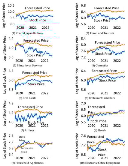
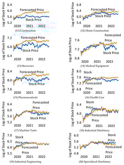
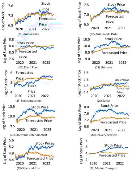
Figure 1.
Actual and predicted Japanese stock prices since the COVID-19 pandemic began. Note: The blue line represents actual sector or firm stock prices and the orange line represents forecasted sector or firm stock prices. Forecasted stock prices are obtained from a regression of sector or firm stock returns on (1) the return on the Japanese stock market, (2) the return on the world stock market, (3) the change in the log of the yen/dollar exchange rate, and (4) the change in the log of the dollar spot price of Dubai crude oil. The regressions are run over the period from 8 April 2010 to 24 February 2020. Actual out-of-sample values of the right-hand side variables are then used to forecast stock prices (the orange line) over the period from 25 February 2020 to 8 February 2023. Source: Datastream database and calculations by the author.
The worst-performing sector in Figure 1 is Central Japan Railways (Panel 1). Stock prices fell immediately in 2020 as travel by train and shinkansen tumbled. Matsuura and Saito (2022) reported that Central Japan Railways continued to supply services during the pandemic but that demand for travel tumbled. Actual stock prices remained 53 percent below predicted values in February 2023. Sakurai and Nakagawa (2023) reported that 70 percent of local railway operators do not expect passenger volume to return to pre-pandemic levels. This drop occurred because remote work has depressed ridership. Many routes may thus be closed.
The second worst-performing sector is travel and tourism (Panel 2). Actual stock prices in this sector were almost 50 percent below predicted values in February 2023. Like train companies, travel agencies have been decimated by travel restrictions. H.I.S. Travel and other agencies suffered as the Tokyo Olympics took place without tourists, and as uncertainty from the pandemic, the Russia–Ukraine War, inflation, and other factors suppressed travel. At the 2021 Tokyo Game Show, H.I.S. provided virtual tours for gamers around the world free of charge rather than organizing trips and receiving remuneration as they had at previous shows (Nagumo 2021).
Educational services (Panel 3) also suffered. Actual stock prices remained more than 40 percent below predicted values at the end of the sample period. COVID-19 restrictions and the shortage of foreign students have decimated their profitability. Much education turned to online delivery. Though there has been demand for this, it often remains unprofitable (Imahashi 2021).
The cosmetics sector (Panel 4) is also performing badly, with stock prices 39 percent below predicted values in February 2023. The sector underperformed as people huddled at home during the 2020 COVID-19 restrictions in Japan and also suffered from stringent restrictions in China. Inflation has also hurt the cosmetics sector, as consumers who are spending more on necessities such as food have had to cut back on cosmetics purchases (Masuda 2022).
Real estate (Panel 5) has also been hit. Stock prices in 2023 remain 36 percent below predicted values. The states of emergency restricted transactions. The demand for office real estate also fell as many worked from home. Restaurants and bars (Panel 6) suffered during the original COVID-19 restrictions and remain 20 percent below predicted values in February 2023. Airlines (Panel 7) and hotels (Panel 8), after underperforming for much of the COVID-19 period, have since recovered. Stock prices are now at or above forecasted levels.
Household appliances (Panel 9) initially performed well and electronic office equipment (Panel 10) initially performed poorly. This is to be expected, as people huddling at home invested more in their homes and firms with empty offices invested less in office equipment. By February 2023, however, household appliance firms performed as expected and office equipment firms performed better than expected.
The construction sector (Panel 11) and the home construction sector (Panel 12) have underperformed. This underperformance is more evident for the overall construction sector than for the home construction sector, reflecting the fact that demand for office buildings has plummeted.
Breweries (Panel 13) have performed poorly. This mirrors the poor performance of restaurants and bars, and the fact that people are going out less. The medical equipment (Panel 14), pharmaceuticals (Panel 15), and health care (Panel 16) sectors all performed well initially as the pandemic began. By February 2023, however, all were underperforming.
Panels 17 through 22 show the performance of key sectors of the Japanese economy (machine tools, industrial machinery, industry engineering, specialized machinery, automobiles, and auto parts). Stock prices for all of them are up from when the pandemic hit and they are all performing as expected.
Panel 23 shows the retail food sector and Panel 24 shows Shimano, a leading bicycle parts maker. Retail foods performed well in 2020, reflecting Aruga’s (2022) finding that there was only a small decrease in visits to grocery stores during the states of emergency. Starting in 2022, as inflation and the weak yen raised costs and as grocery stores did not raise prices commensurately, profits declined. Shimano performed better than forecasted in 2020 and 2021, as many spurned public transportation and opted to bike instead. More recently, Shimano is performing as predicted.
Panel 25 shows the semiconductor sector and Panel 26 banks. When news arrived of the pandemic spreading, it caused many manufacturers such as automakers to cancel orders for chips. Japanese semiconductor stocks fell by 30 percent. Then, as individuals began working from home, they increased spending on computers and other information and communication technologies (ICT). This caused the demand for chips to soar. Demand further increased as people turned from public transportation to automobiles and automakers scrambled to reorder chips. By 2022, soaring demand caused Japanese chipmakers to perform much better than predicted. Banks initially underperformed, but by February 2023, stock prices were 39 percent more than predicted.
The real winners during the pandemic were electronic entertainment (Panel 27), delivery services (Panel 28), steel and iron (Panel 29), and marine transport (Panel 30). As people cloistered at home, demand for computer games and similar technologies soared. This provided a boom for electronic entertainment providers. Delivery services also performed well as many spent more time at home and avoided going out. Steel and iron performed well as steel prices increased almost fourfold between March 202 and February 2023. Marine transport outperformed as soaring demand for ICT and other goods caused shipping rates to rise. The Baltic Dry Index reflects that shipping freight costs increased 11-fold between May 2020 and October 2021.
4. Evidence from Exports, Imports, and Primary Income Flows
4.1. Data and Methodology
Sato et al. (2013) used a vector autoregression (VAR) to investigate how exchange rates impact Japanese exports. A VAR is a regression of an n by 1 vector of endogenous variables, yt, on lagged values of itself:
yt = A1yt-1 + … + Apyt-p + εt, E(εtεt’) = ∑.
Inverting Equation (2) yields an infinite-vector moving average process:
yt = εt + C1εt-1 + C2εt-2 + C3εt-3 + …
The error terms in εt can be contemporaneously correlated. To obtain orthogonalized innovations, the Cholesky factorization can be employed. This method requires finding a lower triangular matrix P such that ∑ = PP’, where ∑ is the variance–covariance matrix of εt. Equation (3) can then be rewritten as:
where Γi = CiP, υt = P−1εt, and E[υtυt’] = I. The endogenous variables in Equation (4) are thus represented as functions of the orthogonalized residuals.
yt = PP−1εt + C1PP−1εt-1 + C2PP−1εt-2 + … = Γ0υt + Γ1υt-1 + Γ2υt-2 + …
Sato et al. (2013), in their three-variable VAR, employed monthly data on industrial production in Japan’s trading partners, the real exchange rate, and exports. Their specification is consistent with the imperfect substitutes model, where exports are a function of the real exchange rate and trading partners’ output (see, e.g., Rose 1991). In the imperfect substitutes framework, imports are a function of the real exchange rate and domestic output. This paper also includes crude oil prices in the VAR.5
This paper uses monthly data and four-variable VARs. The focus of this section is on comparing the performance of exports, imports, and primary income flows with forecasted values. For forecasting, the ordering of the variables does not matter.
The section also reports responses of exports, imports, and primary income flows to shocks to exchange rates and industrial production. For impulse response functions, the ordering of the variables in Equation (4) can make a difference. For exports, the variables are ordered as follows: the spot price of Dubai crude oil, industrial production in OECD countries, real exports, and the real exchange rate. The assumption is that within a month, the variables that are ordered prior can affect the variables that are ordered after but cannot be affected by them. Placing the exchange rate after real exports assumes that exchange rates cannot affect exports within the month. This assumption is reasonable as it takes a little time for exporters to change behavior in response to exchange rate changes.
For imports, the variables in Equation (4) are ordered as follows: the spot price of Dubai crude oil, Japanese industrial production, real imports, and the real exchange rate. Again, placing exchange rates after real imports makes sense as it takes a little time for importers to respond to exchange rate changes. For net income flows from abroad, the variables are ordered as follows: the spot price of Dubai crude oil, OECD industrial production, net income flows, and the real exchange rate.
Data on the spot price of Dubai crude oil come from the Federal Reserve Bank of St. Louis FRED database. Data on OECD and Japanese industrial production come from the OECD GDP database. Data on Japanese real exports and imports of goods and services come from the CEIC database. Data on the broad Japanese real effective exchange rate come from the Bank for International Settlements. Data on net primary income flows come from the Japanese Ministry of Finance. The data are all seasonally adjusted except for the oil price and exchange rate data that do not need seasonal adjustment.
The data on primary income flows are available beginning in January 1996. The VAR is estimated over the period from January 1996 to December 2019. Actual out-of-sample values of the variables are then used to forecast real exports, real imports, and net income flows over the period from January 2020 to December 2022. For forecasting, the ordering of the variables does not matter.
Those variables that augmented Dickey–Fuller (ADF) tests indicate have a unit root are entered in the first-differenced form. Those variables that ADF tests indicate are stationary are entered in levels.
4.2. Results
Panel 1 of Figure 2 shows the response of real exports to an appreciation of the real effective exchange rate. Panel 1 indicates that an appreciation reduces exports, with the effect peaking after five months. Panel 2 shows the response of exports to OECD industrial production. An increase in OECD industrial production raises Japanese exports. The response remains statistically significant for all 24 months.6
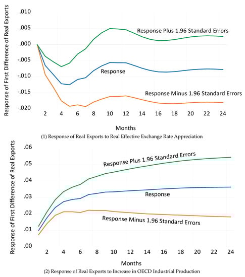
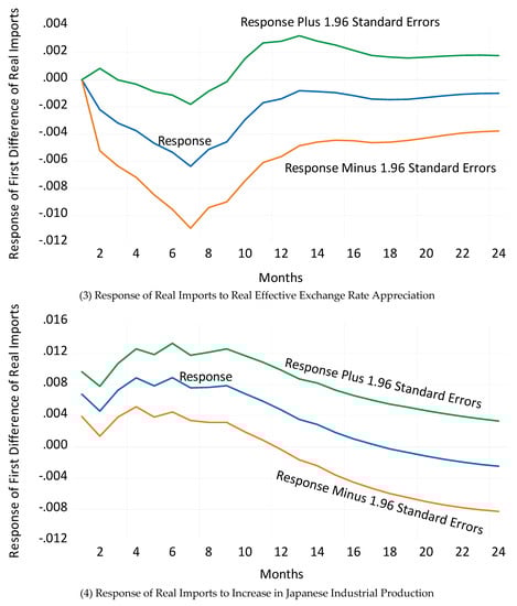
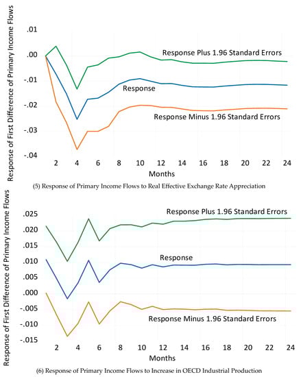
Figure 2.
Impulse Response Functions for Japanese Exports, Imports, and Primary Income Flows. Note: The blue line represents coefficients obtained from the matrices Γi obtained from the orthogonalized moving average processes: yt = Γ0υt + Γ1υt-1 + Γ2υt-2 + … where yt and υt are (4 × 1) vectors. For Japanese exports, the elements of yt are the first difference of the spot price of Dubai crude oil, the first difference of OECD industrial production, the first difference of Japanese real exports of goods and services, and the first difference of the Japanese real effective exchange rate. For Japanese imports, the elements of yt are the first difference of the spot price of Dubai crude oil, Japanese industrial production, the first difference of Japanese real imports of goods and services, and the first difference of the Japanese real effective exchange rate. For Japanese primary income flows, the elements of yt are the first difference of the spot price of Dubai crude oil, the first difference of OECD industrial production, the first difference of Japanese primary income flows deflated by the Japanese CPI, and the first difference of the Japanese real effective exchange rate. The order of the variables in yt are the same as listed above. The data extend from January 1996 to December 2019. The original vector autoregression includes a constant and six lags. The blue lines represent accumulated responses to one standard deviation shocks to the real exchange rate or industrial production. The green and red lines represent 95 percent confidence intervals. All variables are measured in natural logs. Source: Datastream database, Federal Reserve Bank of St. Louis FRED database, OECD GDP database, Japanese Ministry of Finance, Bank for International Settlements, and calculations by the author.
Panels 3 and 4 show the response of real imports to exchange rate appreciations and Japanese industrial production. An appreciation reduces real imports. Thorbecke (2022) reported that an appreciation increases Japanese goods imports and reduces Japanese services imports by more. Since Panel 3 includes both goods and services, the negative impact of an appreciation on services may explain why the overall response is negative. Panel 4 indicates that an increase in Japanese industrial production raises Japanese imports, and the response is statistically significant for the first 12 months.
Panel 5 shows the response of primary income flows to an exchange rate appreciation. The response peaks after 4 months and is statistically significant for most of the 24 months. The response makes sense, as the Japanese yen value of repatriated earnings decreases as the yen appreciates. Panel 6 shows that an increase in OECD industrial production increases primary income, although the response is not statistically significant.
Panel 1 of Figure 3 shows that real exports fell 26 percent between February and May 2020. The figure shows that exports fell much more than forecasted. By October 2020, however, exports had returned to their predicted values. They then remained close to forecasted values until the end of 2022.
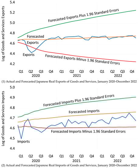
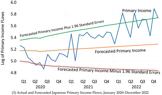
Figure 3.
Forecasted and Actual Values of Japanese Exports, Imports, and Primary Income Flows, January 2020 to December 2022. Note: The blue line represents the actual values of Japanese real goods and services exports (Panel 1), real goods and services imports (Panel 2), and net income flows (Panel 3). The orange line comes from forecasts obtained from a vector autoregression: yt = A1yt-1 + … + Apyt-p + εt. For Japanese real goods and services exports in Panel 1, the elements of yt are the first difference of the spot price of Dubai crude oil, the first difference of OECD industrial production, the first difference of Japanese real exports of goods and services, and the first difference of the Japanese real effective exchange rate. For Japanese real goods and services imports in Panel 2, the elements of yt are the first difference of the spot price of Dubai crude oil, Japanese industrial production, the first difference of Japanese real imports of goods and services, and the first difference of the Japanese real effective exchange rate. For Japanese primary income flows in Panel 3, the elements of yt are the first difference in the spot price of Dubai crude oil, the first difference of OECD industrial production, the first difference of Japanese primary income flows deflated by the Japanese CPI, and the first difference of the Japanese real effective exchange rate. The data extend from January 1996 to December 2019. The original vector autoregression includes a constant and six lags. The green and red lines represent 95 percent confidence intervals around the forecasts. All variables are measured in natural logs. Source: Datastream database, Federal Reserve Bank of St. Louis FRED database, OECD GDP database, Japanese Ministry of Finance, Bank for International Settlements, and calculations by the author.
Panel 2 of Figure 3 shows that real imports fell by 13 percent between January and February 2020. The figure shows that imports were statistically significantly lower than forecasted in February 2020 and again from May through September 2020. After this, imports remained below forecasted values until December 2022. They were no longer statistically significantly below forecasted values, however.
Panel 3 of Figure 3 shows that primary income flows fell 40 percent between January and July 2020. Primary income flows then recovered. For much of 2022, they were statistically significantly more than predicted. High primary income flows in 2022 offset the Japanese trade deficit and kept the overall current account in surplus.
5. Conclusions
The COVID-19 pandemic walloped the Japanese economy. This paper investigated how the Japanese economy is faring three years after its first COVID-19 case by investigating how sectoral and firm stock prices have evolved over these three years compared to forecasts based on the macroeconomic environment. The results indicate that the shinkansen sector, the tourism sector, the education sector, and the cosmetics sector have performed much worse than predicted. Key industries such as machine tools, industrial machinery, industrial engineering, specialized machinery, automobiles, and auto parts, after faring badly when the crisis began, have since rebounded. The electronic entertainment and delivery services sectors, after benefiting from the pandemic, continue to outperform.
This paper also investigates how exports, imports, and net income flows from foreign investments have performed since the pandemic began compared to forecasts based on macroeconomic variables. The findings indicate that exports and imports, after crashing when the pandemic began, are behaving as predicted. Income flows from investments abroad, on the other hand, are outperforming. These repatriated earnings from overseas production are keeping Japan’s current account in surplus even though the increases in the Japanese yen prices of oil and commodity imports have generated trade deficits for 19 consecutive months since August 2021.
The results indicate that the pandemic has caused a long-term drop in stock prices for sectors such as the shinkansen, tourism, education, cosmetics, and others. Croux and Reusens (2013) reported that long-term changes in stock prices have powerful predictive ability for future economic activity. These findings thus point to sustained slowdowns in these sectors. Croux and Reusens also noted that these long-term stock price changes provide useful information for policy makers. Since the travails of these hard-hit industries reflect their exposure to the COVID-19 pandemic rather than mistakes that firms have made, policy makers should consider employing cost-effective ways to stimulate these sectors.7
Funding
The author received no external funding for this research.
Data Availability Statement
The data used in this study are available from the Federal Reserve Bank of St. Louis FRED database, the OECD GDP database, the Japanese Ministry of Finance, the Bank for International Settlements, and the Datastream database.
Acknowledgments
I thank Satoshi Koibuchi, Yuki Masujima, Kiyotaka Sato, Yushi Yoshida, Taiyo Yoshimi, and other colleagues for their excellent comments. Any errors are my own responsibility.
Conflicts of Interest
The author declares no conflict of interest.
Notes
| 1 | These data come from the IMF (2023). |
| 2 | One shortcoming with using market values of stock prices is that they do not necessarily reflect intrinsic value (see Appel and Grabinski 2011). |
| 3 | Papers estimating exchange rate exposures include Bodnar et al. (2002) and Dominguez and Tesar (2006). |
| 4 | The sample starts on 8 April 2010 because this is when daily closing values for the yen/dollar exchange rate could be obtained from Datastream. |
| 5 | I am indebted to Professor Kiyotaka Sato for suggesting that I include crude oil prices in the VAR. |
| 6 | The random variables in the VAR are assumed to follow a Gaussian distribution. As Tormählen et al. (2021) discussed, assuming that random variables are Gaussian is a simplifying assumption that may cloud inference. Future work should explore deriving other distributions. |
| 7 | As an example, Matsuura and Saito (2022) have discussed cost-effective ways that the government has sought to stimulate tourism. |
References
- Appel, Dominik, and Michael Grabinski. 2011. The origin of financial crisis: A wrong definition of value. Portuguese Journal of Quantitative Methods 2: 33–51. [Google Scholar]
- Aruga, Kentaka. 2021. Changes in human mobility under the COVID-19 Pandemic and the Tokyo fuel market. Journal of Risk and Financial Management 14: 163. [Google Scholar] [CrossRef]
- Aruga, Kentaka. 2022. Effects of the human-mobility change during the COVID-19 Pandemic on electricity demand. Journal of Risk and Financial Management 15: 422. [Google Scholar] [CrossRef]
- Bodnar, Gordon M., Bernard Dumas, and Richard C. Marston. 2002. Pass-through and exposure. Journal of Finance 57: 199–231. [Google Scholar] [CrossRef]
- Chan, Kam, and Terry Marsh. 2020. The Asset Markets and the Coronavirus Pandemic. VoxEU Weblog, April 3. Available online: https://www.voxeu.org (accessed on 5 May 2020).
- Chatelais, Nicolas, Arthur Stalla-Bourdillon, and Menzie Chinn. 2023. Forecasting real activity using cross- sectoral stock market information. Journal of International Money and Finance 131: 102800. [Google Scholar] [CrossRef]
- Croux, Christophe, and Peter Reusens. 2013. Do stock prices contain predictive power for the future economic activity? A Granger causality analysis in the frequency domain. Journal of Macroeconomics 35: 93–103. [Google Scholar] [CrossRef]
- Dominguez, Kathryn, and Linda Tesar. 2006. Exchange rate exposure. Journal of International Economics 68: 188–218. [Google Scholar] [CrossRef]
- Fama, Eugene, and Kenneth French. 1993. Common risk factors in the returns on stocks and bonds. Journal of Financial Economics 33: 3–56. [Google Scholar] [CrossRef]
- Gagnon, Joseph, Steven Kamin, and John Kearns. 2023. The impact of the COVID-19 pandemic on global GDP growth. Journal of the Japanese and International Economies. forthcoming. [Google Scholar] [CrossRef]
- Gormsen, Niels, and Ralph Koijen. 2020. Coronavirus: Impact on Stock Prices and Growth Expectations. Thesis, University of Chicago, Chicago, IL, USA. Available online: https://academic.oup.com/raps/article/10/4/574/5904278?login=false (accessed on 15 March 2023).
- Hayakawa, Kazunobu, and Hiroshi Mukunoki. 2021. The impact of COVID-19 on international trade: Evidence from the first shock. Journal of the Japanese and International Economies 60: 101135. [Google Scholar] [CrossRef]
- Hayakawa, Kazunobu, Souknilanh Souknilanh, and Shujiro Urata. 2022. How effective was the restaurant restraining order against COVID-19? A nighttime light study in Japan. Japan and the World Economy 63: 101136. [Google Scholar] [CrossRef] [PubMed]
- Honda, Tomohito, Kaoru Hosono, Daisuke Miyakawa, Arito Ono, and Iichiro Uesugi. 2023. Determinants and effects of the use of COVID-19 business support programs in Japan. Journal of The Japanese and International Economies 67: 101239. [Google Scholar] [CrossRef]
- Imahashi, Rurika. 2021. Japan startups cash in on e-learning demand spurred by COVID. Nikkei Asia, January 6. [Google Scholar]
- IMF. 2023. Japan: Staff Concluding Statement of the 2023 Article IV Mission. January 26. Available online: https://www.imf.org/en/News/Articles/2023/01/25/japan-staff-concluding-statement-of-the-2023-article-iv-mission (accessed on 15 March 2023).
- Kikuchi, Junichi, Ryoya Nagao, and Yoshiyuki Nakazano. 2023. Expenditure responses to the COVID-19 pandemic. Japan and the World Economy 65: 101174. [Google Scholar] [CrossRef] [PubMed]
- Koren, Miklós, and Rita Pető. 2020. Business disruptions from social distancing. In Covid Economics: Vetted and Real-Time Papers 2. London: CEPR Press. Available online: https://cepr.org/content/covid-economics-vetted-and-real-time-papers-0#block-block-10 (accessed on 1 June 2020).
- Kubota, So, Koichiro Onishi, and Yuta Toyama. 2021. Consumption responses to COVID-19 payments: Evidence from a natural experiment and bank account data. Journal of Economic Behavior & Organization 188: 1–17. [Google Scholar]
- Lintner, John. 1965. The valuation of risk assets and the selection of risky investments in stock portfolios and capital budgets. Review of Economics and Statistics 47: 13–37. [Google Scholar] [CrossRef]
- Masuda, Yuki. 2022. Shiseido slashes profit forecast on weak beauty sales in Japan, China. Nikkei Asia, August 11. [Google Scholar]
- Matsuura, Toshiyuki, and Hisamitsu Saito. 2022. The COVID-19 pandemic and domestic travel subsidies. Annals of Tourism Research 92: 103326. [Google Scholar] [CrossRef]
- McMillan, David. 2021. Predicting GDP growth with stock and bond markets: Do they contain different information? International Journal of Finance and Economics 26: 3651–75. [Google Scholar] [CrossRef]
- Nagumo, Jada. 2021. Tokyo Game Show turns to virtual reality in face of COVID. Nikkei Asia, September 29. [Google Scholar]
- Pagano, Marco, Christian Wagner, and Josef Zechner. 2020. Disaster resilience and asset prices. In Covid Economics: Vetted and Real-Time Papers 2. Paris: CEPR Press. Available online: https://arxiv.org/abs/2005.08929 (accessed on 1 June 2020).
- Ramelli, Stefano, and Alexander Wagner. 2020. Feverish stock price reactions to COVID-19. Review of Corporate Finance Studies 9: 622–55. [Google Scholar] [CrossRef]
- Rose, Andrew. 1991. The role of exchange rates in a popular model of international trade: Does the ‘Marshall-Lerner’ condition hold? Journal of International Economics 30: 301–16. [Google Scholar] [CrossRef]
- Sakurai, Yusuke, and Takemi Nakagawa. 2023. 70% of Japan’s local railways say pre-COVID ridership won’t return. Nikkei Asia, May 5. [Google Scholar]
- Sato, Kiyotaka, Junko Shimizu, Nagendra Shrestha, and Shajuan Zhang. 2013. Industry-specific real effective exchange rates and export price competitiveness: The cases of Japan, China, and Korea. Asia Economic Policy Review 8: 298–321. [Google Scholar] [CrossRef]
- Shirai, Sayuri. 2020. Japan’s triple economic shock. East Asia Forum Quarterly 12: 25–26. [Google Scholar]
- Shoji, Masahiro, Susumu Cato, Takashi Iida, Kenji Ishida, Asei Ito, and Kenneth McElwain. 2022. Variations in early-Stage responses to pandemics: Survey evidence from the COVID-19 pandemic in Japan. Economics of Disasters and Climate Change 6: 235–58. [Google Scholar] [CrossRef] [PubMed]
- Thorbecke, Willem. 2019. How oil prices affect East and Southeast Asian economies: Evidence from financial markets and implications for energy security. Energy Policy 128: 628–38. [Google Scholar] [CrossRef]
- Thorbecke, Willem. 2022. Investigating how exchange rates affected the Japanese economy after the advent of Abenomics. Asia and the Global Economy 2: 100028. [Google Scholar] [CrossRef]
- Tormählen, Maike, Galiya Klinkova, and Michael Grabinski. 2021. Statistical significance revisited. Mathematics 9: 958. [Google Scholar] [CrossRef]
Disclaimer/Publisher’s Note: The statements, opinions and data contained in all publications are solely those of the individual author(s) and contributor(s) and not of MDPI and/or the editor(s). MDPI and/or the editor(s) disclaim responsibility for any injury to people or property resulting from any ideas, methods, instructions or products referred to in the content. |
© 2023 by the author. Licensee MDPI, Basel, Switzerland. This article is an open access article distributed under the terms and conditions of the Creative Commons Attribution (CC BY) license (https://creativecommons.org/licenses/by/4.0/).