Derivative of Reduced Cumulative Distribution Function and Applications

Abstract

The reduced cumulative distribution function (rCDF) is the maximal lower bound for the cumulative distribution function (CDF). It is equivalent to the inverse of the conditional value at risk (CVaR), or one minus the buffered probability of exceedance (bPOE). This paper introduces the reduced probability density function (rPDF), the derivative of rCDF. We first explore the relation between rCDF and other risk measures. Then we describe three means of calculating rPDF for a distribution, depending on what is known about the distribution. For functions with a closed-form formula for bPOE, we derive closed-form formulae for rPDF. Further, we describe formulae for rPDF based on a numerical bPOE when there is a closed-form formula for CVaR but no closed-form formula for bPOE. Finally, we give a method for numerically calculating rPDF for an empirical distribution, and compare the results with other methods for known distributions. We conducted a case study and used rPDF for sensitivity analysis and parameter estimation with a method similar to the maximum likelihood method.

1. Introduction

The cumulative distribution function (CDF) and its derivative, the probability density function (PDF), are two of the most important notions in the classical analysis of random variables (see, e.g., Evans and Rosenthal 2004). This paper introduces and explores the reduced probability density function (rPDF), which is the derivative of the reduced cumulative distribution function (rCDF). rCDF, as well as the closely related buffered cumulative distribution function (bCDF), was recently introduced by Grechuk et al. (2023) for multidimensional random variables:

Definition 1.

For any random vector, $\mathbf{X}\in {\mathcal{L}}^{1,n}(\Omega )$, the buffered cumulative distribution function (bCDF) and the reduced cumulative distribution function (rCDF) are given by

$${\overline{F}}_{\mathbf{x}}\left(\mathbf{X}\right)=\underset{\mathbf{a}ϵ{\mathbb{R}}_{+}^n}{inf}E{[{\mathbf{a}}^T\left(\mathbf{x}-\mathbf{X}\right)+1]}^{+},$$

(1)

$${\underline{F}}_{\mathbf{x}}\left(\mathbf{X}\right)=\underset{\mathbf{a}ϵ{\mathbb{R}}_{+}^n}{sup}E\left[min\{1,a_1\left(x_1-X_1\right),\dots ,a_n\left(x_n-X_n\right)\}\right]$$

(2)

respectively, where $\mathbf{a}=(a_1,\dots ,a_n)$, ${\mathbf{a}}^T\mathbf{X}={\sum }_{i=1}^n{a}_i{X}_i$, and ${\mathbb{R}}_{+}^n=\{\mathbf{a}ϵ{\mathbb{R}}^n,\mathbf{a}\ge 0\}$.

For the one-dimensional random variable X, the rCDF considered in this paper reduces to

$${\underline{F}}_x\left(X\right)=\underset{aϵ{\mathbb{R}}_{+}^n}{sup}E\left[min\{1,a\left(x-X\right)\}\right]$$

(3)

and is shown by Grechuk et al. (2023) to be equivalent to the inverse of the conditional value at risk (CVaR) or one minus the buffered probability of exceedance (bPOE). It is thus also equivalent to the super CDF that was earlier considered by Rockafellar and Royset (2014). rPDF completely defines the distribution of a random variable, but unlike the standard probability density function (PDF), it may be focused on a tail of the distribution, allowing us to describe the distribution while measuring different characteristics. This has the potential to be useful in many areas, such as finance and insurance, as well as engineering and systems analysis, as we are often interested in modeling extreme events, which, while rare, can have significant impacts when they do occur. We develop the concept of rPDF as a parallel to the standard PDF in a similar way to which CVaR was developed as a parallel for value at risk (VaR) in Rockafellar and Uryasev (2002), the inverse of CVaR was developed as a parallel for the cumulative distribution function (CDF) in Rockafellar and Royset (2014), and bPOE was developed as a parallel for probability of exceedance (POE) in Rockafellar and Royset (2010) and Mafusalov and Uryasev (2018). We will derive analytical formulae for rPDF for several distributions that have analytical bPOE formulae (see Norton et al. 2019). We then develop formulae for rPDF in terms of a numerically calculated bPOE for situations when an analytical formula for CVaR is known, and give an example. We also develop a general approach for numerically calculating rPDF when no information is available about the distribution of the data.

We conducted two case studies. First, we demonstrated how to use rPDF in sensitivity analysis for a previously considered CDO structuring problem from the perspective of the issuing bank. Second, we examined the use of rPDF in place of standard PDF for finding parameters of a distribution with a technique similar to maximum likelihood estimation, which we call reduced maximum likelihood estimation (rMLE).

Because rPDF is derived from the CVaR concept, which is intended to perform risk management in various applications, we expect that rPDF will be beneficial in the same areas where CVaR is used. At this time, a prime application of CVaR is in financial applications, but it is becoming more and more popular in other areas. These include risk analysis in supply chain management, development of new materials, analysis of large physical systems, nuclear safety, and energy. The sensitivity analysis and rMLE applications presented here are just two of many potential applications of the rPDF concept. The idea of this paper is to attract attention to this new concept, which we are sure will be very useful in various areas similar to the standard PDF so that further research can make use of the concept in additional applications.

2. Background

In various applications, such as engineering and finance, the distributions of random values may not be symmetrical, and often have tails that are fat or long. Characterizing these departures from normality is an important part of managing risk. One popular risk measure, the value at risk (VaR), also known as the quantile, has become an important standard in the financial industry (see Lopez 1997). Defined as

$$q_{\alpha }\left(X\right)=Va{R}_{\alpha }\left(X\right)=min\left\{x\right|\left(P\left(X\right)\le x\right)\ge \alpha \}$$

(4)

for the random variable X and probability $\alpha \in [0,1]$, VaR is the inverse of the cumulative distribution function (CDF) of X, denoted by $F_x\left(X\right)$. This measure gives a value of loss that will only be exceeded a set percentage of the time, $1-\alpha$; however, it tells us little about what the loss could be if it were to exceed the VaR. VaR is also limited in that it lacks useful mathematical properties, such as subadditivity, convexity, and continuity, as a function of the confidence level $\alpha$ for discreet distributions. These limitations became apparent quickly after VaR regulations in banking became the standard (see Krause 2003) and spurred a search for superior risk measures.

In order to better represent the risk in the tail and meet the definition of a coherent risk measure as defined by Artzner et al. (1999), Rockafellar and Uryasev (2002) considered the concept of conditional value at risk (CVaR). CVaR can be defined by the minimization formula (see Rockafellar and Uryasev 2002),

$${\overline{q}}_{\alpha }\left(X\right)=CVa{R}_{\alpha }\left(X\right)=\underset{C}{min}\{C+\frac{1}{1-\alpha }E{[X-C]}^{+}\}$$

(5)

where C is a free optimization variable and ${\left[X\right]}^{+}=max\{X,0\}$. Additionally, the minimizer, C, in (5) is equal to the VaR for the same confidence level $\alpha$,

$$q_{\alpha }\left(X\right)=\underset{C}{argmin}\{C+\frac{1}{1-\alpha }E{[X-C]}^{+}\},$$

(6)

so CVaR and VaR are closely related. Note that the minimum set in the CVaR minimization formula may not be unique. Therefore, usually, VaR is considered to be the smallest value in this set. CVaR, in addition to containing information about the losses in the tail, has superior mathematical properties to VaR, which make it possible to use in stochastic optimization. Specifically, CVaR is continuous with respect to $\alpha$, and convex with respect to X, as well subadditive. In finance applications, CVaR is called expected shortfall, which attracted a lot of attention in literature (see, for instance, Acerbi and Tasche (2022) and Föllmer and Schied (2010)), and is usually defined as follows:

$${\overline{q}}_{\alpha }\left(X\right)=\frac{1}{1-\alpha }{\int }_{\alpha }^1{q}_{\beta }\left(X\right)d\beta .$$

(7)

In the case of a continuous variable X, CVaR is the conditional expectation,

$${\overline{q}}_{\alpha }\left(X\right)=E\left[X|X>q_{\alpha }\left(X\right)\right].$$

(8)

In other words, for continuous distributions, the CVaR for a given level of probability $\alpha$ is the expected value of X, if X exceeds the value at risk for the same level of probability.

Closed-form solutions for CVaR for many families of distributions have been developed over the past two decades (see Landsman and Valdez 2003; Norton et al. 2019), and it has been used extensively as a risk measure in fields such as portfolio optimization (see Hepworth et al. 2017; Chennaf and Ben Amor 2023), enterprise risk management (see Mulvey and Erkan 2006), manufacturing logistics (see Ait-Alla et al. 2014), and energy storage (see Tang et al. 2019). Several studies have also compared the effectiveness of VaR and CVaR in optimization, and found favorable results using CVaR. See, for instance, Kibzun and Vagin (2003), Alexander et al. (2006), and Stoyanov et al. (2012) for such comparisons in financial applications.

Frequently, instead of thinking of risk in terms of a value of loss that is exceeded with a certain probability, we may wish to ask with what probability certain values of loss are exceeded. One way to measure this is with probability of exceedance (POE),

$$p_x\left(X\right)=PO{E}_x\left(X\right)=P\left(X\ge x\right)$$

(9)

where x is a given threshold. For continuous distributions, POE can be calculated by using the inverse function of VaR as follows:

$$p_x\left(X\right)=\left\{1-\alpha |q_{\alpha }\left(X\right)=x\right\},$$

(10)

where $\alpha$ is the probability for which x equals the quantile. However, like VaR, POE has several limitations. Primarily, it tells us only how likely exceeding the threshold is, but says nothing about what the loss could be if the threshold is exceeded. We therefore can often make better use of the buffered probability of exceedance (bPOE), first introduced by Rockafellar and Royset (2010) as buffered probability of failure and developed further by Mafusalov and Uryasev (2018). bPOE is defined as

$${\overline{p}}_x\left(X\right)=bPO{E}_x\left(X\right)=\left\{1-\alpha |{\overline{q}}_{\alpha }\left(X\right)=x\right\}=1-{\overline{q}}_{\alpha }^{-1}\left(X\right).$$

(11)

Mafusalov and Uryasev (2018) showed that

$${\overline{p}}_x\left(X\right)=\underset{C\ge 0}{min}E{[C\left(X-x\right)+1]}^{+}=\underset{\gamma <x}{min}\frac{E{[X-\gamma ]}^{+}}{x-\gamma }$$

(12)

i.e., bPOE, similar to CVaR, can be found via a minimization formula. bPOE for a given threshold, x, is the probability with which tail expectation equals x. Therefore, by definition, bPOE takes into account tail events. Mafusalov and Uryasev (2018) proved many important properties of bPOE, including that it is the lowest quasi-convex upper bound on POE, is strictly decreasing on $xϵ[E\left(X\right),sup\left(X\right))$, and is closed and monotonic with respect to the random variable X. These properties make it useful in a variety of applications. For instance, bPOE has recently been used to describe risk faced by financial institutions by Norton (2019), for solving financial optimization problems by Liu et al. (2022), and in a variety of engineering problems by Kouri and Shapiro (2018), Chaudhuri et al. (2022), and Zrazhevsky et al. (2023).

The relationship between rCDF, VaR, CVaR, POE, and bPOE is illustrated in Figure 1. Note that just as POE is equal to 1 minus the inverse of the quantile function, bPOE equals 1 minus the inverse of CVaR.

Figure 1. Density $f_x\left(X\right)$ is a black curve; x is a given threshold; $bPO{E}_x\left(X\right)=$ probability of the tail with the mean value x (shaded in red); $PO{E}_x\left(X\right)=$ probability of the tail exceeding x (striped diagonally in blue); $rCD{F}_x\left(X\right)=$ probability of outcomes not included in the tail (striped horizontally in green); $CVa{R}_{\alpha }\left(X\right)=x$ is the mean value of the tail with probability $\alpha$; $Va{R}_{\alpha }\left(X\right)=$ lower bound of the tail.

Grechuk et al. (2023) introduced the buffered cumulative distribution function (bCDF) for the random vectors with the notation ${\overline{F}}_x\left(\mathbf{X}\right)$, see (1). For a one-dimensional random value X, it is equal to the inverse of the average VaR, given by ${\overline{Q}}_{\alpha }\left(X\right)=\frac{1}{\alpha }{\int }_0^{\alpha }{q}_s\left(X\right)ds={max}_{c\in \mathbb{R}}\left(c-\frac{1}{\alpha }E{\left[c-X\right]}^{+}\right)$. That is, ${\overline{F}}_x\left(X\right)=\alpha$ when ${\overline{Q}}_{\alpha }\left(X\right)=x$. Grechuk et al. (2023) showed that ${\overline{F}}_x\left(X\right)$ is the minimal quasi-convex upper bound of CDF, $F_x\left(X\right)$. The same paper also defines the reduced cumulative distribution function (rCDF), ${\underline{F}}_{\mathbf{x}}\left(\mathbf{X}\right)$; for random vectors, see (2). For a one-dimensional random variable, this function coincides with the so-called super CDF, defined by Rockafellar and Royset (2014). In this one-dimensional case, ${\underline{F}}_x\left(X\right)=CVa{R}_{\alpha }^{-1}\left(X\right)=1-{\overline{p}}_x\left(X\right)$, which is a maximal quasi-concave lower bound of the CDF (Grechuk et al. 2023). These two bounds of CDF are also shown to be related as follows:

$${\overline{F}}_x\left(X\right)=1-{\underline{F}}_{-x}\left(-X\right),$$

(13)

$${\underline{F}}_x\left(X\right)=1-{\overline{F}}_{-x}\left(-X\right).$$

(14)

This paper is focused on the analysis of rCDF, ${\underline{F}}_x\left(X\right)$. For the standard CDF, $F_x\left(X\right)$, the derivative, $f_x\left(X\right)=\frac{d}{dx}{F}_x\left(X\right),$ is called the probability density function. Similarly, we call the derivative of rCDF the reduced probability density function (rPDF).

Definition 2.

For a random variable, $X\in {\mathcal{L}}^1(\Omega )$, the reduced probability density function (rPDF) at a threshold, x, is given by

$${\underline{f}}_x\left(X\right)=\frac{d}{dx}{\underline{F}}_x\left(X\right)={\underline{F}}_x^{{}^{\prime }}\left(X\right)$$

(15)

where ${\underline{F}}_x\left(X\right)={sup}_{aϵ{\mathbb{R}}_{+}^n}E[min\{1,a\left(x-X\right)\}]={\overline{q}}_x^{-1}\left(X\right)=1-{\overline{p}}_x\left(X\right)$ is the reduced cumulative distribution function (rCDF).

We also call the derivative of bCDF the buffered probability density function (bPDF).

Definition 3.

For a random variable, $X\in {\mathcal{L}}^1(\Omega )$, the buffered probability density function (bPDF) at a threshold, x, is given by

$${\overline{f}}_x\left(X\right)=\frac{d}{dx}{\overline{F}}_x\left(X\right)={\overline{F}}_x^{{}^{\prime }}\left(X\right)$$

(16)

where ${\overline{F}}_x\left(X\right)={inf}_{aϵ{\mathbb{R}}_{+}^n}E{[a^T\left(x-X\right)+1]}^{+}$ is the buffered cumulative distribution function (bCDF).

By differentiating (13) and (14) with respect to x, we can see that rPDF and bPDF are also closely related, as follows:

$${\overline{f}}_x\left(X\right)={\underline{f}}_{-x}\left(-X\right)$$

(17)

We focus only on rPDF in this paper, as bPDF can be easily computed from rPDF.

Note also that by using the alternate definition of rCDF, we see that rPDF is the negative of the derivative of bPOE as shown below:

$${\underline{f}}_x\left(X\right)={\underline{F}}_x^{{}^{\prime }}\left(X\right)={\left(1-{\overline{p}}_x\left(X\right)\right)}^{{}^{\prime }}=-{\overline{p}}_x^{{}^{\prime }}\left(X\right).$$

(18)

3. Calculating rPDF

This section examines several approaches for calculating rPDF, depending on what information is available about the distribution for which we wish to find it.

3.1. rPDF for Distributions with Closed-Form bPOE

We begin by looking at four distributions for which closed-form solutions for bPOE are known. These formulae were derived by Norton et al. (2019) for the exponential, Pareto, generalized Pareto, and Laplace distributions.

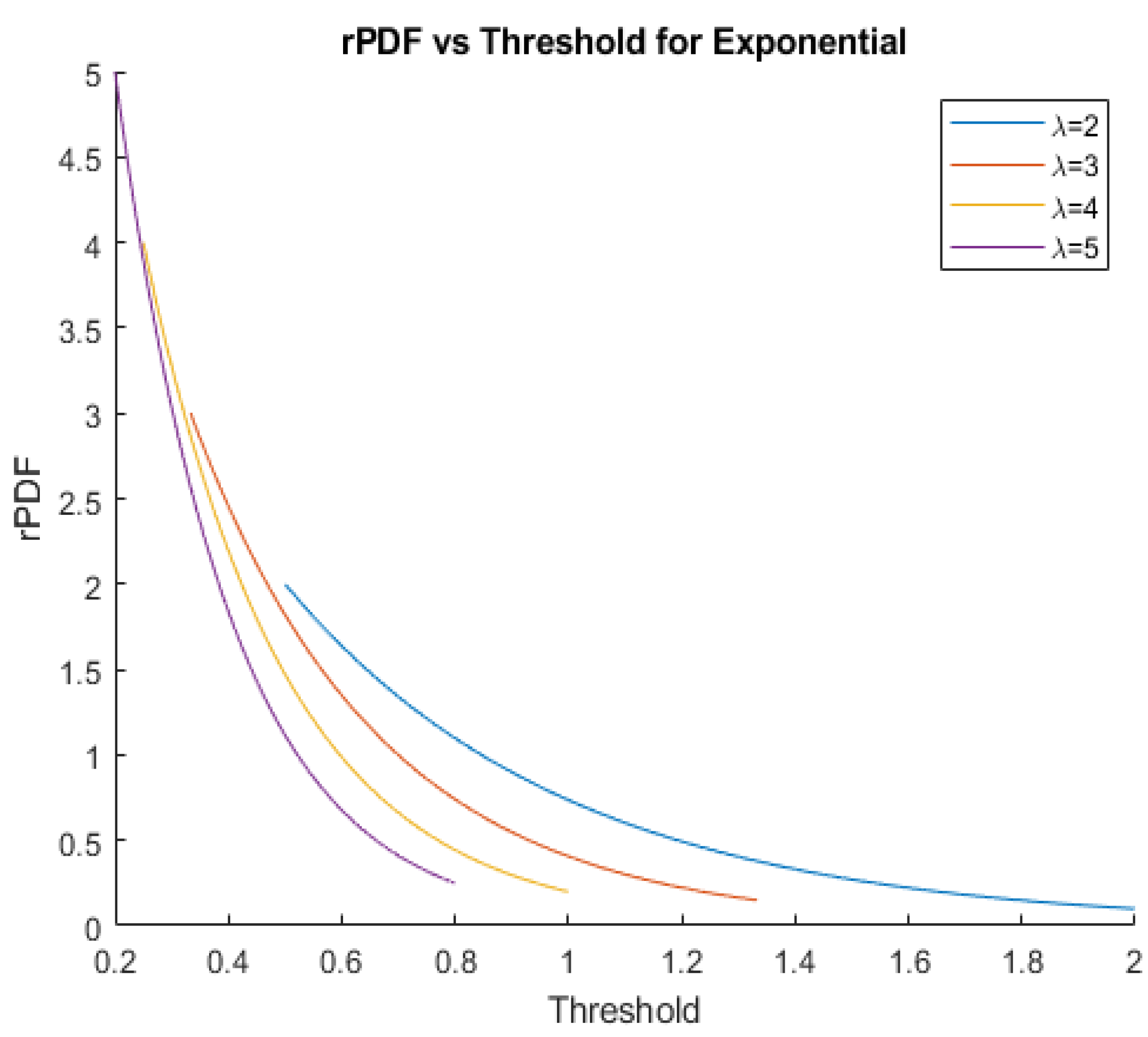
3.1.1. The Exponential Distribution

For the exponential distribution, with PDF and CDF given by

$$f\left(x\right)=\left\{\begin{array}{cc}\lambda e^{-\lambda x}\hfill & x\ge 0\hfill \\ 0\hfill & x<0\hfill \end{array}\right.$$

(19)

and

$$F\left(x\right)=\left\{\begin{array}{cc}1-e^{-\lambda x}\hfill & x\ge 0\hfill \\ 0\hfill & x<0\hfill \end{array}\right.$$

(20)

respectively, the bPOE function is (see Norton et al. 2019)

$${\overline{p}}_x\left(X\right)=e^{1-\lambda x}.$$

(21)

By taking the derivative and negating it, we obtain rPDF.

Proposition 1.

Let $X\sim exponential\left(\lambda \right)$. Then,

$${\underline{f}}_x\left(X\right)=\lambda e^{1-\lambda x}$$

(22)

Proof. 

$${\underline{f}}_x\left(X\right)=-\frac{d{\overline{p}}_x\left(X\right)}{dx}=\lambda e^{1-\lambda x}$$

□

Figure 2 shows graphs of rPDF for exponential distribution.

Figure 2. rPDFs for exponential distributions with several values of $\lambda$.

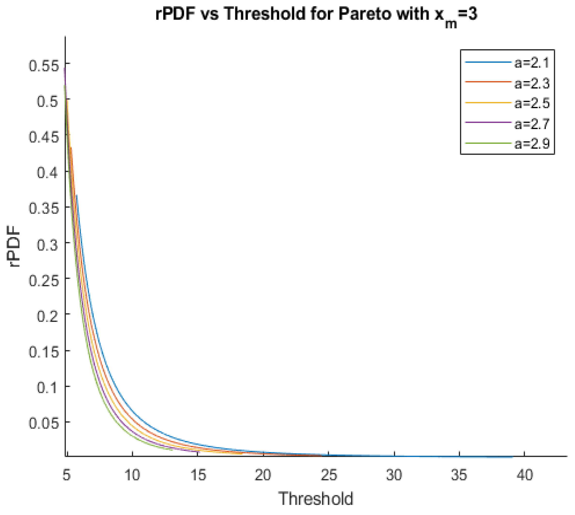
3.1.2. The Pareto Distribution

For the Pareto distribution with PDF and CDF given by

$$f\left(x\right)=\left\{\begin{array}{cc}\frac{a{x}_m^a}{x^{a+1}}\hfill & x\ge x_m\hfill \\ 0\hfill & x<x_m\hfill \end{array}\right.$$

(23)

and

$$F\left(x\right)=\left\{\begin{array}{cc}1-{\left(\frac{x_m}{x}\right)}^a\hfill & x\ge x_m\hfill \\ 0\hfill & x<x_m\hfill \end{array}\right.$$

(24)

bPOE is (see Norton et al. (2019))

$${\overline{p}}_x\left(X\right)={\left(\frac{x_{m}a}{x\left(a-1\right)}\right)}^a.$$

(25)

Proposition 2.

For $X\sim Pareto(a,x_m)$, rPDF is

$${\underline{f}}_x\left(X\right)=\frac{x_m^a{a}^{a+1}}{{\left(a-1\right)}^a}·\frac{1}{x^{a+1}}$$

(26)

Proof. 

$${\overline{p}}_x\left(X\right)={\left(\frac{x_{m}a}{x\left(a-1\right)}\right)}^a={\left(\frac{x_{m}a}{\left(a-1\right)}\right)}^a{x}^{-a}$$

$${\underline{f}}_x\left(X\right)=-\frac{d{\overline{p}}_x\left(X\right)}{dx}=\frac{x_m^a{a}^{a+1}}{{\left(a-1\right)}^a}·\frac{1}{x^{a+1}}$$

□

Figure 3 shows graphs of the rPDF function for several Pareto distributions with various values of a, all with the same position parameter, $x_m=3$.

Figure 3. rPDFs for Pareto distributions with several values of a and $x_m=3$.

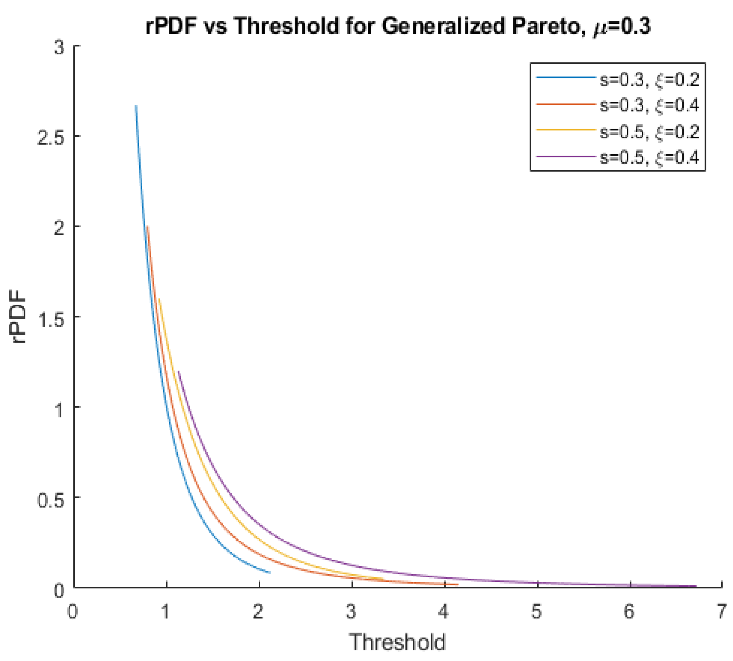
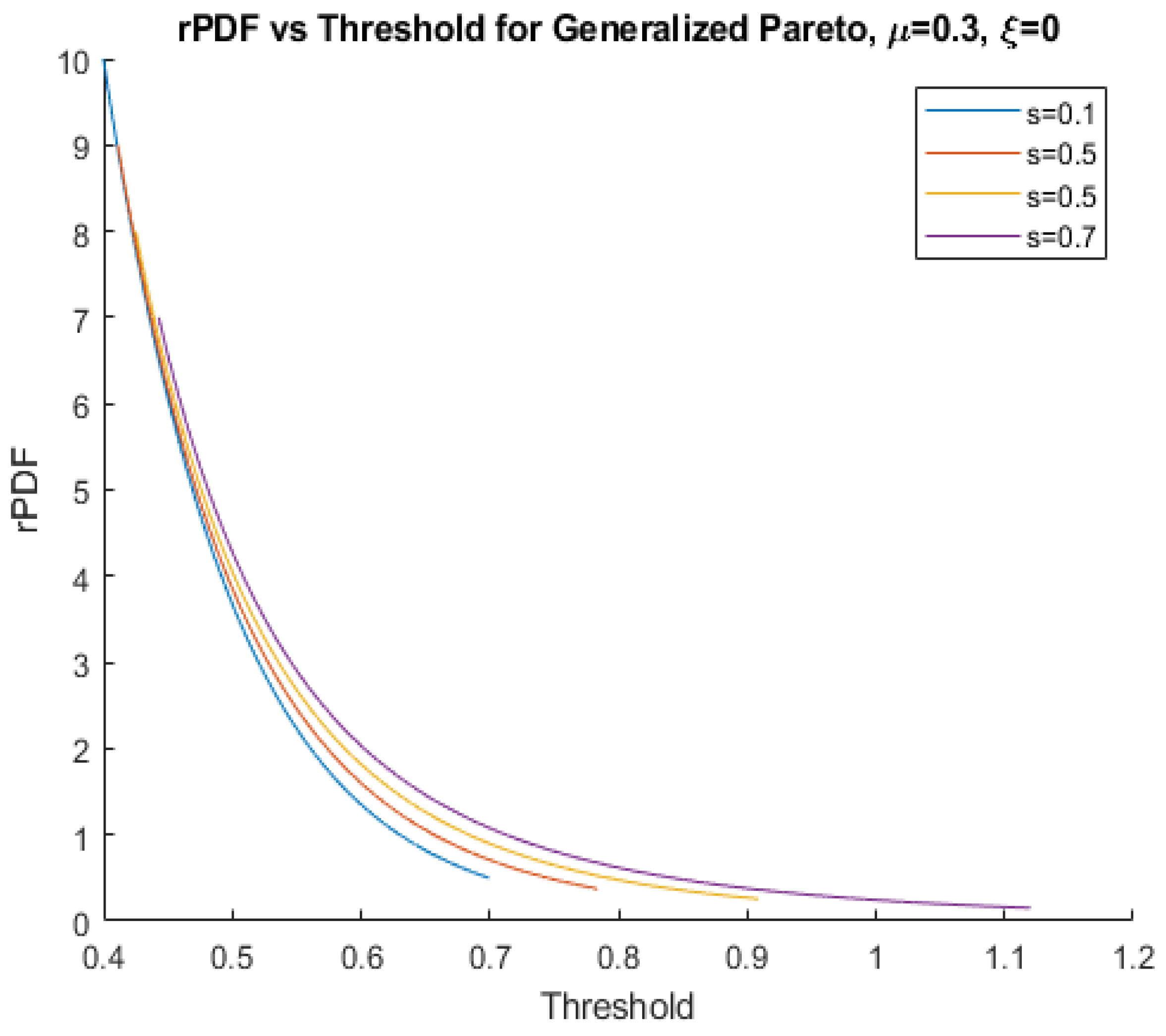
3.1.3. The Generalized Pareto Distribution

For a three-parameter generalized Pareto distribution with PDF and CDF given by

$$f\left(x\right)=\frac{1}{s}{\left(1+\frac{\xi \left(x-\mu \right)}{s}\right)}^{\frac{-1}{\xi }-1}$$

(27)

and

$$F\left(x\right)=\left\{\begin{array}{cc}1-{\left(1+\frac{\xi \left(x-\mu \right)}{s}\right)}^{\frac{-1}{\xi }}\hfill & \xi \ne 0\hfill \\ 1-e^{-\left(\frac{x-\mu }{s}\right)}\hfill & \xi =0\hfill \end{array}\right.$$

(28)

where $\mu$ is the location parameter, s the scale parameter, and $\xi$ the shape parameter, the bPOE given by Norton et al. (2019) is

$${\overline{p}}_x\left(X\right)=\left\{\begin{array}{cc}\frac{{\left(1+\frac{\xi \left(x-\mu \right)}{s}\right)}^{\frac{-1}{\xi }}}{{(1-\xi )}^{\frac{1}{\xi }}}\hfill & \xi \ne 0\hfill \\ e^{1-\left(\frac{x-\mu }{s}\right)}\hfill & \xi =0\hfill \end{array}\right.$$

(29)

Taking the derivative and negating it for each branch, we find rPDF:

Proposition 3.

For $X\sim generalizedPareto(\mu ,s,\xi )$, rPDF is

$${\underline{f}}_x\left(X\right)=\left\{\begin{array}{cc}\frac{{\left(1+\frac{\xi \left(x-\mu \right)}{s}\right)}^{\frac{-1}{\xi }-1}}{s{\left(1-\xi \right)}^{\frac{1}{\xi }}}\hfill & \xi \ne 0\hfill \\ \frac{1}{s}{e}^{1-\left(\frac{x-\mu }{s}\right)}\hfill & \xi =0\hfill \end{array}\right.$$

(30)

Proof. 

$${\underline{f}}_x\left(X\right)=-\frac{d{\overline{p}}_x\left(X\right)}{dx}=\left\{\begin{array}{cc}\frac{{\left(1+\frac{\xi \left(x-\mu \right)}{s}\right)}^{\frac{-1}{\xi }-1}}{s{\left(1-\xi \right)}^{\frac{1}{\xi }}}\hfill & \xi \ne 0\hfill \\ \frac{1}{s}{e}^{1-\left(\frac{x-\mu }{s}\right)}\hfill & \xi =0\hfill \end{array}\right.$$

□

We will assume that $\xi <0.5$ as, otherwise, the established formulae for the moments of the distribution do not hold. Figure 4 shows graphs of the rPDF function for several generalized Pareto distributions with various values of s and $\xi$, all with the same position parameter, $\mu$ = 0.3, while Figure 5 shows graphs for generalized Pareto distributions with various values of s when $\mu$ = 0.3 and $\xi =0$.

Figure 4. rPDFs for generalized Pareto distributions with several values of s and $\xi$ and $mu$ = 0.3.

Figure 5. rPDFs for generalized Pareto distributions with several values of s when $\xi =0$ and $mu$ = 0.3.

3.1.4. The Laplace Distribution

For a Laplace distribution with PDF and CDF given by

$$f\left(x\right)=\frac{1}{2b}{e}^{\frac{-|x-\mu |}{b}}$$

(31)

and

$$F\left(x\right)=\left\{\begin{array}{cc}1-\frac{1}{2}{e}^{\frac{-\left(x-\mu \right)}{b}}\hfill & x\ge \mu \hfill \\ \frac{1}{2}{e}^{\frac{x-\mu }{b}}\hfill & x<\mu \hfill \end{array}\right.$$

(32)

where $\mu$ and b are location and scale parameters, bPOE equals (see Norton et al. 2019)

$${\overline{p}}_x\left(X\right)=\left\{\begin{array}{cc}\frac{1}{2}{e}^{1-\frac{x-\mu }{b}}\hfill & x\ge \mu +b\hfill \\ 1+\frac{z}{W(-2e^{-z-1}z)}\hfill & x>\mu +b\hfill \end{array}\right.$$

(33)

where $z=\frac{x-\mu }{b}$ and $W\left(x\right)$ is the Lambert-W function.

Proposition 4.

For $X\sim Laplace\left(\mu ,b\right)$, with $z=\frac{x-\mu }{b}$, bPDF is

$${\underline{f}}_x\left(X\right)=\left\{\begin{array}{cc}\frac{1}{2b}{e}^{1-\frac{x-\mu }{b}}\hfill & x\ge \mu +b\hfill \\ \frac{-W\left(-2e^{-z-1}z\right)\frac{1}{b}+z\frac{W\left(-2e^{-z-1}z\right)}{\left(-2e^{-z-1}z\right)\left(1+W\left(-2e^{-z-1}z\right)\right)}\left(\frac{-2}{b}{e}^{-z-1}+\frac{2}{b}z{e}^{-z-1}\right)}{{\left(W\left(-2e^{-z-1}z\right)\right)}^2}\hfill & x<\mu +b\hfill \end{array}\right.$$

(34)

Proof. 

For the case $x\ge \mu +b$, the proof is trivial:

$${\underline{f}}_x\left(X\right)=-\frac{d{\overline{p}}_x\left(X\right)}{dx}=\frac{1}{2b}{e}^{1-\frac{x-\mu }{b}}.$$

For the case $x<\mu +b$, we utilize the derivative of the Lambert-W function, $\frac{dW\left(x\right)}{dx}=\frac{1}{x+e^{W\left(x\right)}}$. Since $z=\frac{x-\mu }{b}$,$\frac{dz}{dx}=\frac{1}{b}$, the expression for ${\underline{f}}_x\left(X\right)$ follows from the chain rule. □

3.2. rPDF for Distributions with Closed-Form CVaR

Many distributions do not have an analytical expression for bPOE. However, many common distributions do have an analytical expression for CVaR; see Norton et al. (2019). With these formulae, and remembering that ${\underline{f}}_x\left(X\right)=-{\overline{p}}_x^{{}^{\prime }}\left(X\right)={\left({\overline{q}}_x^{-1}\left(X\right)\right)}^{{}^{\prime }}$, we can use the following rule for taking the derivative of the inverse of a function, even without knowing ${\overline{q}}_x^{-1}\left(X\right)$:

$${\left(f^{-1}\left(x\right)\right)}^{{}^{\prime }}=\frac{1}{f^{{}^{\prime }}\left(f^{-1}\left(x\right)\right)}$$

(35)

For our purposes, $f\left(x\right)$ is the CVaR. We can calculate $f^{-1}\left(x\right)$ by first calculating bPOE numerically from a given data set at the necessary threshold value, and then using the fact that ${\overline{q}}_x^{-1}\left(X\right)=1-$${\overline{p}}_x\left(X\right)$. For numerical calculations, we have used the PSG package AORDA (2022). Thus, we find rPDF by using the following:

Proposition 5.

$${\left({\overline{q}}_x^{-1}\left(X\right)\right)}^{{}^{\prime }}=\frac{1}{{\overline{q}}_{1-{\overline{p}}_x\left(X\right)}^{{}^{\prime }}\left(X\right)}$$

(36)

where ${\overline{q}}_{1-{\overline{p}}_x\left(X\right)}^{{}^{\prime }}\left(X\right)$ is the derivative of ${\overline{q}}_{\alpha }\left(X\right)$ with respect to α, and $1-{\overline{p}}_x\left(X\right)$ then plugged in for α.

Normal Distribution

As an example, we take the normal distribution, whose CVaR is given in Norton et al. (2019):

$${\overline{q}}_{\alpha }\left(X\right)=\mu +\sigma \frac{\phi \left({\Phi }^{-1}\left(\alpha \right)\right)}{1-\alpha },$$

(37)

where $\mu$ is the mean, $\sigma$ is the standard deviation, $\phi \left(x\right)=\frac{1}{\sqrt{2\pi }}{e}^{\frac{-x^2}{2}}$, ${\Phi }^{-1}\left(x\right)=\sqrt{2}er{f}^{-1}(2x-1)$, and $er{f}^{-1}\left(x\right)$ is the inverse error function, whose derivative (derived using (35)) is $\frac{d}{dx}er{f}^{-1}\left(x\right)=\frac{\sqrt{\pi }}{2}{e}^{{\left(er{f}^{-1}\left(x\right)\right)}^2}$.

Corollary 1.

$${\underline{f}}_x\left(X\right)=\frac{\sqrt{2\pi }}{\sigma }\frac{{\left(1-\left(1-{\overline{p}}_x\left(X\right)\right)\right)}^2}{-2\sqrt{\pi }\left(1-\left(1-{\overline{p}}_x\left(X\right)\right)\right)\left(er{f}^{-1}\left(2\left(1-{\overline{p}}_x\left(X\right)\right)-1\right)\right)+e^{-{\left(er{f}^{-1}(2(1-{\overline{p}}_x\left(X\right))-1)\right)}^2}}$$

(38)

Proof. 

Taking the derivative of ${\overline{q}}_{\alpha }\left(X\right)$ with respect to $\alpha$ gives

$$\frac{d{\overline{q}}_{\alpha }\left(X\right)}{d\alpha }=\frac{\sigma }{\sqrt{2\pi }}\frac{-2\sqrt{\pi }\left(1-\alpha \right)\left(er{f}^{-1}\left(2\alpha -1\right)\right)+e^{-{\left(er{f}^{-1}(2\alpha -1)\right)}^2}}{{\left(1-\alpha \right)}^2}$$

Using (36) then gives

$${\left({\overline{q}}_x^{-1}\left(X\right)\right)}^{{}^{\prime }}=\frac{\sqrt{2\pi }}{\sigma }\frac{{\left(1-\left(1-{\overline{p}}_x\left(X\right)\right)\right)}^2}{-2\sqrt{\pi }\left(1-(1-{\overline{p}}_x\left(X\right))\right)\left(er{f}^{-1}\left(2(1-{\overline{p}}_x\left(X\right))-1\right)\right)+e^{-{\left(er{f}^{-1}(2(1-{\overline{p}}_x\left(X\right))-1)\right)}^2}}$$

(39)

which is equivalent to the rPDF, ${\underline{f}}_x\left(X\right)$. □

This process is also replicable for other distributions with closed-form CVaRs but no closed-form bPOEs, such as the student-t and log-normal distributions.

3.3. rPDF at Given Values When the Distribution Is Unknown or Has No Closed-Form CVaR Formula

If we do not have a closed-form formula for the CVaR of a distribution, or we do not know what distribution a set of data comes from, as is generally the case in financial applications, we can still find a value for the rPDF at a given value for the threshold. To achieve this, we use a formula for the derivative of ${\overline{q}}_{\alpha }\left(X\right)$ with respect to $\alpha$, given in Rockafellar and Uryasev (2002) in which they detail the properties of CVaR:

$$\frac{\partial {\overline{q}}_{\alpha }\left(X\right)}{\partial \alpha }=\frac{1}{{\left(1-\alpha \right)}^2}E\left({\left[X-q_{\alpha }\left(X\right)\right]}^{+}\right).$$

(40)

By substituting $1-{\overline{p}}_x\left(X\right)$ for $\alpha$ in (40), calculating numerically both bPOE at the given threshold, and VaR at one minus this bPOE, and combing this with (36), we obtain a formula for the value of the rPDF at the threshold.

Proposition 6.

$${\underline{f}}_x\left(X\right)=\frac{{\left({\overline{p}}_x\left(X\right)\right)}^2}{E\left({\left[X-q_{1-{\overline{p}}_x\left(X\right)}\left(X\right)\right]}^{+}\right)}.$$

(41)

Proof. 

$${\left({\overline{q}}_x^{-1}\left(X\right)\right)}^{{}^{\prime }}=\frac{1}{{\overline{q}}_{1-{\overline{p}}_x\left(X\right)}^{{}^{\prime }}\left(X\right)}=\frac{1}{\frac{1}{{\left({\overline{p}}_x\left(X\right)\right)}^2}E\left({\left[X-q_{1-{\overline{p}}_x\left(X\right)}\left(X\right)\right]}^{+}\right)},$$

$${\underline{f}}_x\left(X\right)={\left({\overline{q}}_x^{-1}\left(X\right)\right)}^{{}^{\prime }}=\frac{{\left({\overline{p}}_x\left(X\right)\right)}^2}{E\left({\left[X-q_{1-{\overline{p}}_x\left(X\right)}\left(X\right)\right]}^{+}\right)}.$$

□

We note that this result is consistent with the partial derivatives of bPOE described in Zhang et al. (2019), although our approach to the problem is different.

4. Application 1: Sensitivity Analysis for bPOE and rCDF Optimization

One potential application of rPDF lies in sensitivity analysis. bPOE has recently become a popular risk measure in fields such as portfolio optimization, insurance, and classification, due to bPOE’s quasi-convexity with respect to the random variable. In optimization, bPOE constraints have been previously shown to be equivalent to CVaR constraints (Norton et al. 2019), but any given bPOE constraint also has an equivalent rCDF constraint since rCDF is one minus bPOE. For example, the constraint

$${\overline{p}}_x\left(X\right)\le c$$

(42)

is equivalent to the constraint

$${\underline{F}}_x\left(X\right)\ge 1-c.$$

(43)

Thus, for any optimization problem involving a constraint on bPOE, the problem could also be stated in terms of rCDF. As rPDF is the derivative of rCDF with respect to the threshold, we can use rPDF to estimate the sensitivity of the rCDF function (and that of the bPOE function) around a given value for the threshold. We demonstrate this in the following financial case study. Note, however, that such sensitivity analysis can be used to perform risk management in many areas, such as the risk of failure of nuclear systems or of building materials. The rate of change of the buffered failure probability is found using rPDF.

Case Study: Optimal Step-Up CDO Structuring

For this case study, we use real data considered by a major British bank in a problem on determining the optimal structure for a step-up collateralized debt obligation (CDO), which was previously examined by Pertaia et al. (2021). The CDO is assumed to have five tranches: a senior tranche, three mezzanine tranches, and an equity tranche. The problem seeks to structure the CDO using selections from up to 58 credit default swaps (CDSs). Data contain lists of CDS defaults and the recovery rates in 300,000 scenarios. One way of achieving the optimal structure studied in Pertaia et al. (2021) is to constrain the probability of default of each tranche. This is performed by including an upper bound on the bPOE for the maximum cumulative loss of each tranche minus its attachment point at a threshold of zero (where a difference greater than zero indicates default). Alternatively, we could use an equivalent constraint for rCDF.

In some scenarios, however, we may be interested in the probability of the loss at some other threshold close to but not equal to zero. We can use rPDF to assess the sensitivity of rCDF to small changes in the threshold, around a given threshold value. For example, for the first tranche of the CDO in this case study, the bPOE is equal to 0.06653 at a threshold of $x=0$, which gives an rCDF of 0.93347 for the same threshold. We can numerically calculate the rPDF at this threshold, using the technique described in (41), as we know that the bPOE is ${\overline{p}}_0\left(X\right)=0.06653$ and the VAR is easily calculated from the list of maximum cumulative losses at the corresponding threshold to be $q_{1-0.06653}\left(X\right)=-0.02312$. We find an rPDF of ${\underline{f}}_0\left(X\right)=2.87766$, where X represents the maximum cumulative loss minus the attachment point of the tranche. We can then use this value as the slope in a linear approximation of the rCDF as a function of the threshold, centered at $(0,0.93347)$:

$${\underline{\widehat{F}}}_x\left(X\right)=2.87766\left(x-0\right)+0.93347$$

(44)

Table 1 shows directly calculated rCDF values at thresholds close to zero compared with the estimates provided by this linear approximation.

Table 1. Exact values of rCDF and estimates found using linear approximation centered at $(0,0.93347)$.

x	−0.01	−0.001	−0.0001	0	0.0001	0.001	0.01
${\underline{F}}_x\left(X\right)$	0.88863	0.93046	0.93318	0.93347	0.93375	0.93632	0.95796
${\underline{\widehat{F}}}_x\left(X\right)$	0.90469	0.93059	0.93318	0.93347	0.93375	0.93634	0.96224

We can similarly analyze the sensitivity of bPOE to changes in the threshold, because rPDF is negative of the derivative of bPOE. Again looking at the first tranche of the CDO, we can approximate the value of bPOE for thresholds near zero using

$${\widehat{\overline{p}}}_x\left(X\right)=-2.87766\left(x-0\right)+0.06653$$

(45)

since the bPOE for a threshold of zero was 0.06653.

The more rapidly decreasing accuracy of approximations for thresholds below zero compared with that for thresholds above zero can be explained by the curvature of the rCDF and bPOE curves with respect to the threshold. Both are steeper for values below zero than for values above zero, as shown in Figure 6 and Figure 7.

Figure 6. The rCDF for the first tranche of the CDO at various thresholds, x is displayed in blue, and the tangent line (with slope equal to rPDF) at the point where $x=0$ in red.

Figure 7. The bPOE for the first tranche of the CDO at various thresholds, x is displayed in blue, and the tangent line (with slope equal to −1 times rPDF) at the point where $x=0$ in red.

This is in turn because rPDF values for this data set are more extreme for thresholds below zero, as seen in Figure 8. Similar results were seen for the other tranches of the CDO.

Figure 8. The rPDF for the first tranche of the CDO at various thresholds, x.

5. Application 2: Reduced Maximum Likelihood Estimation Using Closed-Form rPDF Formulae

Maximum likelihood estimation (MLE) is a popular method of parameter estimation that has long been used in a wide variety of fields (see, for instance, Millar (2011), Nagelkerke (2012), Ward and Ahlquist (2018)). For the distributions studied in Section 3.1, we here develop optimization problems based on MLE, but using rPDF in place of PDF. We call this reduced maximum likelihood estimation (rMLE). These problems are used with simulated data in the following case study. We demonstrate that rMLE estimates parameters with a reasonable accuracy. We also compare these results with those found using the standard MLE technique, and find that they are similar.

5.1. The Exponential Distribution

We can use (22) to find a reduced maximum likelihood estimator for $\lambda$. We find the reduced likelihood function, $\underline{L}\left(\lambda ;x_1,\dots ,x_n\right)$, and then reduced log-likelihood function, $\underline{l}\left(\lambda ;x_1,\dots ,x_n\right)$, and maximize the latter. These are calculated in the same way as the standard likelihood and log-likelihood functions, but using rPDF instead of PDF.

Corollary 2.

For $X\sim exponential\left(\lambda \right)$, the rMLE estimator of λ calculated using ${\underline{f}}_x\left(X\right)$ is

$$\widehat{\lambda }=\frac{1}{\overline{x}}$$

(46)

Proof. 

$$\underline{L}\left(\lambda ;x_1,\dots ,x_n\right)=\prod _{i=1}^n{\underline{f}}_x\left(x_i;\lambda \right)=\prod _{i=1}^n\lambda e^{1-\lambda x_i}={\lambda }^n{e}^{n-\lambda {\sum }_{i=1}^n\left(x_i\right)},$$

$\underline{l}\left(\lambda ;x_1,\dots ,x_n\right)=ln\left({\lambda }^n{e}^{n-\lambda {\sum }_{i=1}^n\left(x_i\right)}\right)=nln\left(\lambda \right)+n-\lambda {\sum }_{i=1}^n\left(x_i\right)$. Taking the partial derivative with respect to $\lambda$ and solving, we obtain

$$\frac{\partial \underline{l}}{\partial \lambda }=\frac{n}{\lambda }-\sum _{i=1}^n\left(x_i\right)=0,$$

$$\widehat{\lambda }=\frac{n}{{\sum }_{i=1}^n\left(x_i\right)}=\frac{1}{\overline{x}}.$$

□

Notably, this is the same estimator we would obtain by maximizing the standard log-likelihood function, obtained from the PDF of an exponential distribution.

5.2. The Pareto Distribution

Using (26) for the rPDF of a Pareto distribution, we find the following reduced likelihood and reduced log-likelihood and their gradients.

Corollary 3.

For a Pareto random variable, X, the reduced likelihood and reduced log-likelihood based on rPDF are

$$\underline{L}\left(a,x_m;x_1,\dots ,x_n\right)=\prod _{i=1}^n{\underline{f}}_x\left(x_i;a,x_m\right)=\prod _{i=1}^n\frac{x_m^a{a}^{a+1}}{{\left(a-1\right)}^a}·\frac{1}{x_i^{a+1}}=\frac{x_m^{an}{a}^{an+n}}{{\left(a-1\right)}^{an}}\prod _{i=1}^n\frac{1}{x_i^{a+1}}$$

(47)

and

$$\underline{l}\left(a,x_m;x_1,\dots ,x_n\right)=ln\underline{L}\left(a,x_m;x_1,\dots ,x_n\right)$$

$$=anln\left(x_m\right)+\left(an+n\right)ln\left(a\right)-anln\left(a-1\right)-(a+1)\sum _{i=1}^{n}ln\left(x_i\right)$$

(48)

with log-likelihood gradients

$$\frac{\partial \underline{l}}{\partial a}=nln\left(x_m\right)+\frac{\left(an+n\right)}{a}+nln\left(a\right)-\frac{an}{\left(a-1\right)}-nln\left(a-1\right)-\sum _{i=1}^{n}ln\left(x_i\right)$$

(49)

and

$$\frac{\partial \underline{l}}{\partial x_m}=\frac{an}{x_m}.$$

(50)

It should be noted that because the reduced log-likelihood is monotonically increasing with respect to $x_m$, the reduced maximum likelihood will occur when $x_m$ is at its highest possible value, which is the minimum of the original observations. The result for an a value, however, is more complicated. The reduced log-likelihood function is monotonically decreasing with respect to a for $a>1$, implying that the optimal value is $a=1$. The observations being used in the reduced likelihood function are CVaRs, which are bounded on the left by the expected value. Since the expected value of a Pareto distribution is given by $E\left[X\right]=\frac{a{x}_m}{a-1}$, we can use the following inequality to constrain the possible values of a:

$$E\left[X\right]=\frac{a{x}_m}{a-1}\le x_{min},$$

(51)

where $x_{min}$ is the smallest of the CVaR observations. By solving the previous inequality for a, we obtained the following constraint:

$$a\ge \frac{x_{min}}{x_{min}-x_m}$$

(52)

This constraint allows for finding an a value maximizing reduced log-likelihood, after choosing the smallest observation ${\widehat{x}}_m$ as our estimate of $x_m$, by solving the following problem.

Problem 1.

$$\underset{a}{max}\left(anln\left({\widehat{x}}_m\right)+\left(an+n\right)ln\left(a\right)-anln\left(a-1\right)-\left(a+1\right)\sum _{i=1}^{n}ln\left(x_i\right)\right)$$

(53)

$$s.t.a\ge \frac{x_{min}}{x_{min}-{\widehat{x}}_m}$$

5.3. The Generalized Pareto Distribution

For the generalized Pareto distribution, we use (30) to develop two separate reduced log-likelihood functions, one for when $\xi \ne 0$ and one for when $\xi =0$.

Corollary 4.

In the case where $\xi \ne 0$, the reduced likelihood and reduced log-likelihood are

$$\underline{L}\left(\mu ,s,\xi ;x_1,\dots ,x_n\right)=\frac{1}{s^n{\left(1-\xi \right)}^{\frac{n}{\xi }}}\prod _{i=1}^n{\left(1+\frac{\xi \left(x_i-\mu \right)}{s}\right)}^{\frac{-1}{\xi }-1},$$

(54)

$$\underline{l}\left(\mu ,s,\xi ;x_1,\dots ,x_n\right)=-nln\left(s\right)-\frac{n}{\xi }ln\left(1-\xi \right)+\left(\frac{-1}{\xi }-1\right)\sum _{i=1}^{n}ln\left(1+\frac{\xi \left(x_i-\mu \right)}{s}\right),$$

(55)

and the reduced log-likelihood has gradients:

$$\frac{\partial \underline{l}}{\partial \mu }=(1+\xi )\sum _{i=1}^n\left(\frac{1}{s+\xi \left(x_i-\mu \right)}\right),$$

(56)

$$\frac{\partial \underline{l}}{\partial s}=\frac{-n}{s}+(1+\xi )\sum _{i=1}^n\left(\frac{x_i-\mu }{s^2+s\xi \left(x_i-\mu \right)}\right),$$

(57)

$$\frac{\partial \underline{l}}{\partial \xi }=\frac{n}{\xi (1-\xi )}+\frac{n}{{\xi }^2}ln\left(1-\xi \right)+\left(\frac{-1}{\xi }-1\right)\sum _{i=1}^n\left(\frac{x_i-\mu }{s+\xi \left(x_i-\mu \right)}\right)+\frac{1}{{\xi }^2}\sum _{i=1}^{n}ln\left(1+\frac{\xi \left(x_i-\mu \right)}{s}\right).$$

(58)

Proof. 

$$\underline{L}\left(\mu ,s,\xi ;x_1,\dots ,x_n\right)=\prod _{i=1}^n{\underline{f}}_x\left(x_i;\mu ,s,\xi \right)=\frac{1}{s^n{\left(1-\xi \right)}^{\frac{n}{\xi }}}\prod _{i=1}^n{\left(1+\frac{\xi \left(x_i-\mu \right)}{s}\right)}^{\frac{-1}{\xi }-1},$$

$$\underline{l}\left(\mu ,s,\xi ;x_1,\dots ,x_n\right)=ln\left(\frac{1}{s^n{\left(1-\xi \right)}^{\frac{n}{\xi }}}\prod _{i=1}^n{\left(1+\frac{\xi \left(x_i-\mu \right)}{s}\right)}^{\frac{-1}{\xi }-1}\right)$$

$$=-nln\left(s\right)-\frac{n}{\xi }ln\left(1-\xi \right)+\left(\frac{-1}{\xi }-1\right)\sum _{i=1}^{n}ln\left(1+\frac{\xi \left(x_i-\mu \right)}{s}\right),$$

$$\frac{\partial \underline{l}}{\partial \mu }=\left(\frac{-1}{\xi }-1\right)\sum _{i=1}^n\left(\frac{-\frac{\xi \left(x_i-\mu \right)}{s}}{1+\frac{\xi \left(x_i-\mu \right)}{s}}\right)=(1+\xi )\sum _{i=1}^n\left(\frac{1}{s+\xi \left(x_i-\mu \right)}\right),$$

$$\frac{\partial \underline{l}}{\partial s}=\frac{-n}{s}+\left(\frac{-1}{\xi }-1\right)\sum _{i=1}^n\left(\frac{\frac{-\xi \left(x_i-\mu \right)}{s^2}}{1+\frac{\xi \left(x_i-\mu \right)}{s}}\right)=\frac{-n}{s}+(1+\xi )\sum _{i=1}^n\left(\frac{x_i-\mu }{s^2+s\xi \left(x_i-\mu \right)}\right),$$

$$\frac{\partial \underline{l}}{\partial \xi }=\frac{n}{\xi (1-\xi )}+\frac{n}{{\xi }^2}ln\left(1-\xi \right)+\left(\frac{-1}{\xi }-1\right)\sum _{i=1}^n\left(\frac{x_i-\mu }{s+\xi \left(x_i-\mu \right)}\right)+\frac{1}{{\xi }^2}\sum _{i=1}^{n}ln\left(1+\frac{\xi \left(x_i-\mu \right)}{s}\right).$$

□

Corollary 5.

For the case $\xi =0$:

$$\underline{L}\left(\mu ,s,\xi ;x_1,\dots ,x_n\right)=\frac{1}{s^n}\prod _{i=1}^n{e}^{1-\left(\frac{x_i-\mu }{s}\right)},$$

(59)

$$\underline{l}\left(\mu ,s,\xi ;x_1,\dots ,x_n\right)=-nln\left(s\right)+n+\frac{n\mu }{s}+\frac{1}{s}\sum _{i=1}^n\left(x_i\right),$$

(60)

and the log-likelihood has gradients:

$$\frac{\partial \underline{l}}{\partial \mu }=\frac{n}{s},$$

(61)

$$\frac{\partial \underline{l}}{\partial s}=\frac{-n}{s}-\frac{n\mu }{s^2}-\frac{1}{s^2}\sum _{i=1}^n\left(x_i\right),$$

(62)

$$\frac{\partial \underline{l}}{\partial \xi }=0.$$

(63)

Proof. 

$$\underline{L}\left(\mu ,s,\xi ;x_1,\dots ,x_n\right)=\prod _{i=1}^n{\underline{f}}_x\left(x_i;\mu ,s,\xi \right)=\frac{1}{s^n}\prod _{i=1}^n{e}^{1-\left(\frac{x_i-\mu }{s}\right)},$$

$$\underline{l}\left(\mu ,s,\xi ;x_1,\dots ,x_n\right)=ln\left(\frac{1}{s^n}\prod _{i=1}^n{e}^{1-\left(\frac{x_i-\mu }{s}\right)}\right)=-nln\left(s\right)+n+\frac{n\mu }{s}+\frac{1}{s}\sum _{i=1}^n{x}_i.$$

The gradients are straightforward to calculate from here using standard differentiation rules. □

In order to deal with the two cases, since we do not know in advance whether data come from a distribution with $\xi =0$, both reduced log-likelihood functions are maximized. Then, the parameter values corresponding to the maximum log-likelihood are used. We have used PSG (AORDA 2022) to solve the maximization problems.

As with the standard Pareto distribution, we can use the fact that the CVaR values must be greater than or equal to the expected value of the distribution to derive constraints for the maximization problems. For the generalized Pareto, the expected value is given by $E\left(X\right)=\mu +\frac{s}{1-\xi }$. Thus, we have the following:

$$\mu +\frac{s}{1-\xi }\le x_{min},$$

(64)

or equivalently,

$$\left(x_{min}-\mu \right)\xi +s\le x_{min}-\mu ,$$

(65)

where $x_{min}$ is the smallest of the CVaR observations. In the case where $\xi =0$, this simplifies to

$$s\le x_{min}-\mu .$$

(66)

We also note that since $\mu$ is a location parameter, we can treat it similarly to $x_m$ in the standard Pareto case, and use the smallest observation as our estimate, $\widehat{\mu }$. Further, we define Problem 2 and Problem3 to find a reduced maximum likelihood estimate for s and $\xi$ when $\xi \ne 0$, and s when $\xi =0$, respectively.

Problem 2.

$$\underset{s,\xi }{max}-nln\left(s\right)-\frac{n}{\xi }ln\left(1-\xi \right)+\left(\frac{-1}{\xi }-1\right)\sum _{i=1}^{n}ln\left(1+\frac{\xi \left(x_i-\widehat{\mu }\right)}{s}\right)$$

(67)

$$s.t.\left(x_{min}-\widehat{\mu }\right)\xi +s\le x_{min}-\widehat{\mu }$$

$$0<\xi <0.5$$

Problem 3.

$$\underset{s}{max}-nln\left(s\right)+n+\frac{n\widehat{\mu }}{s}-\frac{1}{s}\sum _{i=1}^n{x}_i$$

(68)

$$s.t.s\le x_{min}-\widehat{\mu }$$

5.4. The Laplace Distribution

The Laplace distribution does not lend itself to reduced maximum likelihood estimation, as the rPDF function (see (34)) is piecewise-defined with respect to x. Which branch is used for which observations is dependent on how those observations compare with the parameters. However, it should be noted that if $x\ge \mu +b$ is true for all CVaRs, and the location parameter estimated as the mean of the observations (as in the standard MLE), the estimator for b can be solved for analytically. The estimate is identical to that found with standard MLE, $\widehat{b}=\frac{{\sum }_{i=1}^n(x_i-\widehat{\mu })}{n}$.

Corollary 6.

If $X\sim Laplace\left(\mu ,b\right)$ and $x_i\ge \mu +b$ for all CVaR observations, $x_i$, then the reduced maximum likelihood estimator for b, derived from the rPDF, is

$$\widehat{b}=\frac{{\sum }_{i=1}^n(x_i-\widehat{\mu })}{n}$$

(69)

Proof. 

$$\underline{L}\left(\mu ,b;x_1,\dots ,x_n\right)=\prod _{i=1}^n{\underline{f}}_x\left(x_i;\mu ,b\right)=\frac{1}{2^n{b}^n}{e}^{{\sum }_{i=1}^n\left(1-\frac{x_i-\mu }{b}\right)},$$

$$\underline{l}\left(\mu ,b;x_1,\dots ,x_n\right)=-nln\left(2\right)-nln\left(b\right)+n-\frac{{\sum }_{i=1}^n{x}_i}{b}+\frac{n\mu }{b},$$

$$\frac{\partial \underline{l}}{\partial b}=-\frac{n}{b}+\frac{{\sum }_{i=1}^n\left(x_i-\mu \right)}{b^2}=0,$$

$$b=\frac{{\sum }_{i=1}^n\left(x_i-\mu \right)}{n}.$$

□

6. rMLE Case Study

This section uses simulated data to test some of the theoretically developed results. For the exponential, Pareto, and generalized Pareto distributions, we simulate sets of data points taken from those distributions with known parameters. Further, we solve the optimization problems presented in Section 4 to estimate their parameters using rPDF. We then use data simulated from a normal distribution to demonstrate how to build the rPDF curve for a distribution when CVaR has a closed-form solution but bPOE does not. Finally, we use the same normally distributed data to calculate rPDF numerically at each threshold and compare these results with those found with the CVaR-based approach.

6.1. Exponential Distribution

Although we have an analytical solution for rMLE in this case, we used PSG to find the estimator numerically to confirm our results for observations drawn from an exponential distribution. Using 3000 simulated observations from the exponential distribution with $\lambda =4$, the rMLE was found to be $\widehat{\lambda }=3.9953$. Figure 9 and Figure 10 show the log-likelihood and its gradient vs. values of the parameter $\lambda$, and we observe that the reduced likelihood is maximized very close to 4.

Figure 9. Reduced log-likelihood as a function of the parameter $\lambda$ for the exponential distribution, with the maximum at $\lambda =3.9953$.

Figure 10. Gradient of the log-likelihood (in blue) for the exponential distribution. The gradient crosses the x-axis (in red) at $\lambda =3.9953$.

6.2. Pareto Distribution

We used 3000 simulated observations from an exponential distribution with $a=2.3$ and $x_m=3$. Problem 1 was optimized with PSG. The estimate used for $x_m$ (the smallest original observation) was 3.0009, and the rMLE found for a was 2.3194.

6.3. Generalized Pareto Distribution

We sampled 20,000 observations from a generalized Pareto distribution with $\mu$ = 0.3, s = 0.3, $\xi$ = 0.4. We used PSG to solve Problem 2 and Problem 3 and took the solution with the largest log-likelihood. The estimate used for $\mu$ (the smallest original observation) was 0.3000, the rMLE for s was 0.2994, and the rMLE for $\xi$ was 0.4129.

We then sampled 20,000 observations from a generalized Pareto distribution with $\mu$ = 0.2, s = 0.3, $\xi$ = 0. We again solved Problem 2 and Problem 3 with PSG and took the solution with the largest log-likelihood. The estimate used for $\mu$ (the smallest original observation) was 0.2000, the rMLE for s was 0.2993, and the rMLE for $\xi$ was 0.

6.4. Normal Distribution

To demonstrate the methods for calculating rPDF when there is no closed-form bPOE formula available, we used 2000 observations from a normal distribution with a mean of 3 and a standard deviation of 1.5. First, we used the built-in function in PSG to calculate bPOE values at 2000 threshold values between 3 and 7.5 (that is, between the mean and three standard deviations above the mean). We then used these numerically calculated bPOE values and (38) to find the value of rPDF at each threshold value. The bPOE and rPDF are graphed as functions of the threshold in Figure 11 and Figure 12, respectively.

Figure 11. bPOE vs. threshold for normal (3, 1.5).

Figure 12. rPDF vs. threshold for normal (3, 1.5).

We then used the empirical approach we described in (41) with the same observations to calculate the rPDF at the same threshold values through the following procedure:

• For the chosen threshold, x, calculate the bPOE.
• Calculate the VaR with an $\alpha$ of 1-bPOE.
• Subtract the VaR value from each value in the data set.
• Find the mean of only the positive values.
• Divide the bPOE squared by this mean.

Figure 13 shows the values of rPDF calculated by this method on the same set of axes as that calculated using (38) previously.

Figure 13. rPDF for observations from N(3, 1.5) using the methods described in (38) and (41).

Figure 13 shows that the evaluation procedure produces similar, though less smooth, curve everywhere, except for the threshold where bPOE = 1 (when rPDF is zero). This is due to difficulties in calculating the VaR when $\alpha =0$.

7. Conclusions

This paper introduced the concept of rPDF, and defined it as the derivative of rCDF. To calculate the rPDF, we can use analytical formulae for rCDF. Additionally, we can differentiate the inverse of CVaR, or take the negative of the derivative of bPOE. We used known formulae for bPOE to derive formulae for rPDF for the exponential, Pareto, generalized Pareto, and Laplace distributions. rPDF can be used for sensitivity analysis of stochastic systems. Additionally, we showed how rPDF can be used to conduct reduced MLE (rMLE), a method similar to the standard MLE for the estimation of the parameters of the distributions. We also showed that it is possible to use known closed-form CVaR formulae and numerical calculations of bPOE to find a value for rPDF at a given threshold for a given set of data. We can use VaR and bPOE to approximate rPDF at given thresholds based on an empirical set of data with no distributional assumptions.

We conducted several case studies. Sensitivity analysis was performed for the evaluation of failures of CDO tranches. With rPDF, we analyzed the sensitivity of both rCDF and bPOE to changes in the threshold. In particular, rPDF was used to linearly approximate values of rCDF and bPOE for thresholds close to those for which rCDF or bPOE is known.

When testing the rMLE technique with simulated observations, we achieved results very close to the actual values of the parameters of the distributions from which the observations came. Unfortunately, at this time, we are limited to using rMLE in cases where we have an analytical formula for the bPOE of the relevant distribution, and we only have such formulae for a few distributions. While we have demonstrated methods for calculating the rPDF in other cases, they require us to numerically estimate bPOE values at each threshold, which prevents rMLE from working as it obscures some of rPDF’s dependence on the parameters.

We also used both the CVaR-based formula and the empirical method to generate rPDF curves for observations taken from a normal distribution. The two curves were very similar, indicating that the empirical technique provides a reasonable estimate of the rPDF curve given enough observations.

Potential future work may include a thorough examination of the mathematical properties of rPDF and further development of various applications of rPDF. rPDF may be very useful in financial applications due to rPDF’s focus on the tail, rather than the center of the distributions. For example, rPDF could help to evaluate how securities would react in extreme situations with very high losses. We could apply rPDF-based sensitivity analysis, as demonstrated with the CDO structuring problem here, to any bPOE- or rCDF-based portfolio optimization problem. We are also considering an rPDF-based analog to the Hellinger distance, which we believe could allow us to better identify cases where distributions are similar in their centers but significantly different in their tails. This would allow us, for instance, to identify securities that may behave similarly in normal times but quite differently in times of extreme market stress.

References

- Acerbi, Carlo, and Dirk Tasche. 2022. Expected shortfall: A natural coherent alternative to value at risk. Economic Notes 31: 379–88. [Google Scholar] [CrossRef]
- Ait-Alla, Abderrahim, Michael Teucke, Michael Lütjen, Samaneh Beheshti-Kashi, and Hamid Reza Karimi. 2014. Robust production planning in fashion apparel industry under demand uncertainty via conditional value at risk. Mathematical Problems in Engineering 2014: 901861. [Google Scholar] [CrossRef]
- Alexander, Siddharth, Thomas F. Coleman, and Yuying Li. 2006. Minimizing CVAR and var for a portfolio of derivatives. Journal of Banking & Finance 30: 583–605. [Google Scholar]
- AORDA. 2022. Portfolio Safeguard (PSG). Available online: http://aorda.com/ (accessed on 1 September 2023).
- Artzner, Philippe, Freddy Delbaen, Jean-Marc Eber, and David Heath. 1999. Coherent measures of risk. Mathematical Finance 9: 203–28. [Google Scholar] [CrossRef]
- Chaudhuri, Anirban, Boris Kramer, Matthew Norton, Johannes O. Royset, and Karem Willcox. 2022. Certifiable risk-based engineering design optimization. AIAA Journal 60: 551–65. [Google Scholar] [CrossRef]
- Chennaf, Souad, and Jaleleddine Ben Amor. 2023. Mean-CVAR portfolio optimization models based on chance theory. International Journal of Information Technology & Decision Making 22: 1–35. [Google Scholar]
- Evans, Michael J., and Jeffrey S. Rosenthal. 2004. Probability and Statistics: The Science of Uncertainty. New York: W. H. Freeman. [Google Scholar]
- Föllmer, Hans, and Alexander Schied. 2010. Convex risk measures. Encyclopedia of Quantitative Finance 1: 355–363. [Google Scholar]
- Grechuk, Bogdan, Michael Zabarankin, Alexander Mafusalov, and Stan Uryasev. 2023. Buffered and Reduced Multidimensional Distribution Functions. Optimization Letters. [Google Scholar] [CrossRef]
- Hepworth, Adam J., Michael P. Atkinson, and Roberto Szechtman. 2017. A sequential elimination approach to value-at-risk and conditional value-at-risk selection. Paper presented at the 2017 Winter Simulation Conference (WSC), Las Vegas, NV, USA, December 3–6. [Google Scholar]
- Kibzun, Andrey, and Vadim Vagin. 2003. Comparison of VaR and CVaR Criteria. Automation and Remote Control 64: 1154–64. [Google Scholar] [CrossRef]
- Kouri, Drew P., and Alexander Shapiro. 2018. Optimization of PDEs with Uncertain Inputs. In Frontiers in PDE-Constrained Optimization. New York: Springer Nature, pp. 41–81. [Google Scholar]
- Krause, Andreas. 2003. Exploring the limitations of value at risk: How good is it in practice? The Journal of Risk Finance 4: 19–28. [Google Scholar] [CrossRef]
- Landsman, Zinoviy M., and Emiliano A. Valdez. 2003. Tail conditional expectations for elliptical distributions. North American Actuarial Journal 7: 55–71. [Google Scholar] [CrossRef]
- Liu, Junyi, Ying Cui, and Jong-Shi Pang. 2022. Solving nonsmooth and nonconvex compound stochastic programs with applications to risk measure minimization. Mathematics of Operations Research 47: 3051–83. [Google Scholar] [CrossRef]
- Lopez, Jose A. 1997. Regulatory Evaluation of Value-at-Risk Models. SSRN Electronic Journal. Available online: https://papers.ssrn.com/sol3/papers.cfm?abstract_id=1577 (accessed on 1 September 2023).
- Mafusalov, Alexander, and Stan Uryasev. 2018. Buffered probability of exceedance: Mathematical Properties and Optimization. SIAM Journal on Optimization 28: 1077–103. [Google Scholar] [CrossRef]
- Millar, Russell B. 2011. Maximum Likelihood Estimation and Inference: With Examples in R, SAS and ADMB. Chichester: Wiley. [Google Scholar]
- Mulvey, John M., and Hafize G. Erkan. 2006. Applying CVaR for decentralized risk management of financial companies. Journal of Banking & Finance 30: 627–44. [Google Scholar]
- Nagelkerke, Nico J. D. 2012. Maximum Likelihood Estimation of Functional Relationships. New York: Springer. [Google Scholar]
- Norton, Matthew. 2019. Assessing Risk of Exceedance Events with Buffered Probability of Exceedance and Superquantiles. Paper presented at 13th International Conference on Applications of Statistics and Probability in Civil Engineering, Seoul, Republic of Korea, May 26–30. [Google Scholar]
- Norton, Matthew, Valentyn Khokhlov, and Stan Uryasev. 2019. Calculating CVaR and bPOE for common probability distributions with application to portfolio optimization and density estimation. Annals of Operations Research 299: 1281–315. [Google Scholar] [CrossRef]
- Pertaia, Giorgi, Artem Prokhorov, and Stan Uryasev. 2021. A new approach to credit ratings. Journal of Banking and Finance 140: 106097. [Google Scholar] [CrossRef]
- Rockafellar, R. Tyrrell, and Johannes O. Royset. 2010. On buffered failure probability in design and optimization of structures. Reliability Engineering & System Safety 95: 499–510. [Google Scholar]
- Rockafellar, R. Tyrrell, and Johannes O. Royset. 2014. Random variables, monotone relations, and convex analysis. Mathematical Programming 148: 297–331. [Google Scholar] [CrossRef]
- Rockafellar, R. Tyrrell, and Stan Uryasev. 2002. Conditional value-at-risk for general loss distributions. Journal of Banking and Finance 26: 1443–71. [Google Scholar] [CrossRef]
- Stoyanov, Stoyan V., Svetlozar T. Rachev, and Frank J. Fabozzi. 2012. Sensitivity of portfolio var and CVAR to portfolio return characteristics. Annals of Operations Research 205: 169–87. [Google Scholar] [CrossRef]
- Tang, Zao, Junyong Liu, Youbo Liu, Yuan Huang, and Shafqat Jawad. 2019. Risk awareness enabled sizing approach for hybrid energy storage system in distribution network. IET Generation, Transmission & Distribution 13: 3814–22. [Google Scholar]
- Ward, Michael D., and John S. Ahlquist. 2018. Maximum Likelihood for Social Science: Strategies for Analysis. Cambridge: Cambridge University Press. [Google Scholar]
- Zhang, Tong, Stan Uryasev, and Yongpei Guan. 2019. Derivatives and subderivatives of buffered probability of exceedance. Operations Research Letters 47: 130–32. [Google Scholar] [CrossRef]
- Zrazhevsky, Grigoriy, Vira Zrazhevska, and Alexander Golodnikov. 2023. Developing a model for a modulating mirror fixed on active supports: Stochastic model. Cybernetics and Systems Analysis 59: 101–7. [Google Scholar] [CrossRef]
Disclaimer/Publisher’s Note: The statements, opinions and data contained in all publications are solely those of the individual author(s) and contributor(s) and not of MDPI and/or the editor(s). MDPI and/or the editor(s) disclaim responsibility for any injury to people or property resulting from any ideas, methods, instructions or products referred to in the content. |
© 2023 by the authors. Licensee MDPI, Basel, Switzerland. This article is an open access article distributed under the terms and conditions of the Creative Commons Attribution (CC BY) license (https://creativecommons.org/licenses/by/4.0/).