Modeling Bivariate Dependency in Insurance Data via Copula: A Brief Study

Abstract

Copulas are a quite flexible and useful tool for modeling the dependence structure between two or more variables or components of bivariate and multivariate vectors, in particular, to predict losses in insurance and finance. In this article, we use the VineCopula package in R to study the dependence structure of some well-known real-life insurance data and identify the best bivariate copula in each case. Associated structural properties of these bivariate copulas are also discussed with a major focus on their tail dependence structure. This study shows that certain types of Archimedean copula with the heavy tail dependence property are a reasonable framework to start in terms modeling insurance claim data both in the bivariate as well as in the case of multivariate domains as appropriate.

1. Introduction

Modeling insurance data via copula is not new in the literature. For example, Alexeev et al. (2021) studied dependence among insurance claims arising from different lines of business via copula. Shi et al. (2016) discussed a multilevel modeling of insurance claims using copula. Pfeifer and Neslehova (2003) discussed at length in a survey paper the role of copula in modeling dependence in finance and insurance. In exploring dependence structures related to insurance (from any business domain, such as healthcare sector, travel industry, etc.) one pertinent aspect is the assessment of various types of risk (for example, portfolio risk) arising out of each of these domains. There is no denying of the fact that without the proper assessment of risk, insurance coverage to public and private property/organization (as the case may be) as well as for individuals associated cannot be evaluated effectively. Consequently, in the literature, there are several instances of using bivariate and/or multivariate copula and studying their tail dependence behavior. For a detailed study on copula and associated bivariate (as well as multivariate) dependence based on copula theory, see the books by Joe (1997) and Nelsen (2006). A non-exhaustive list of such references may be cited as follows. Mensi et al. (2017) has discussed via a wavelet-based copula approach the dependence structure across oil, wheat, and corn. The authors have established time varying asymmetric tail dependence (at different time zones) between the pair of cereals as well as between oil and the two cereals. Naeem et al. (2021) studied the asymmetric and extreme tail dependence between five energy markets and green bonds using a time-varying optimal copula. This serves as a motivation for the current work. In this article, we focus on studying the dependence structure between two components resulting from insurance claim datasets. Specifically, we consider Australian automobile insurance data and the Swedish motor insurance data. There is little or no evidence of studying automobile insurance data that are asymmetric in nature via copula. This is another motivation to carry out this work. These datasets are selected from a wide collection of CAS datasets available in R. Here, we consider a copula-based modeling of insurance claims data, especially the tail dependence and through a specific selection criteria in R, popularly known as the VineCopula package, to select the best fitted copula in each of these datasets. This paper investigates dependence among insurance claims arising from the auto industry with datasets selected from two different countries. Interestingly, for the first dataset, the Australian automobile insurance data, we examine the dependence among (pairwise) four different variables; each such comparison is useful in the context of claims assessed from the insured as well as the insurer. The details are provided in each model description in Section 3. For a detailed study on the use of copula, see Shi et al. (2016) and the references cited therein. The second dataset is taken from two different countries on motor insurance claims. In this case, we study the tail dependence between claims submitted and the number of insured motorists. When modeling dependency between components of insurance claims using copula, we aim to select copulas that are capable of generating upper- and or lower-tail dependence, that is, when several components of the insurance claims have a strong tendency to exhibit extreme losses simultaneously. We expect that the outcomes of this study provide valuable insights with regards to the nature of dependence and satisfy one of the primary objectives of the general insurance providers aiming at assessing total risk of an aggregate portfolio of losses when components of insurance are correlated. General insurance (for example, property–casualty) protects individuals and organizations from financial losses due to property damage or legal liabilities, in our case, due to auto accident. Consequently, it allows policyholders to exchange the risk of a large loss for the certainty of smaller periodic payments of premiums. Next, insurers allocates the bulk of premium dollars into investment and claims payments. As it is for an insurer to manage its investment portfolio, it is equally important for the insurer to manage its claim portfolio. It is the counterpart of asset management for the claims on the insurer’s book. Claim management is the analytics of insurance costs. It requires applying statistical techniques in the analysis and interpretation of the claims data. In the data-driven industry of general insurance, claim management provides useful insights for insurers to make better business decisions. From the above, it is quite evident as to why a study of insurance claims via copula is important.

In this article, we aim to model the dependence structure (in the bivariate domain) of data arising out of financial domains, precisely, from the insurance domain via copula. Insurance data from the automobile sector are selected for these purposes that are asymmetric in nature. We consider the application of vine copulas (in two dimensions) for several types of insurance data which are asymmetric in nature by utilizing the Vine Copula package in R. It appears that the resultant most appropriate bivariate copulas are members of the C and D-vine copulas, and among them, some are Archimedean as well. A vine copula is a copula constructed from a set of $\frac{d\left(d-1\right)}{2}$ bivariate copulas by using successive mixing according to a tree structure on finite indexes $1,\cdots ,d$. Depending on the types of trees, various vine copulas can be constructed. The remainder of the paper is organized as follows. In Section 2, we discuss some basic definitions and useful preliminaries on copula theory. In Section 3, we discuss in details two different datasets, subsequently fitting an appropriate bivariate copula to each of them. In Section 4, we discuss some useful structural properties of these copulas, in particular tail dependence structures that are pertinent in the study of insurance claims dependence structure. Finally, some concluding remarks are made in Section 5.

2. Bivariate Copula and Its Properties

We begin this section by reviewing some basic definitions and concepts related to copula. The utility of Sklar’s theorem is that the modeling of the marginal distributions can be conveniently and efficiently separated from the dependence modeling in terms of the copula. Interestingly, the major task that lies in practical applications is how to identify this copula. For the bivariate case, a rich collection of copula families is available and well-investigated (see, for details, Joe 1997; Nelsen 2006). Sklar’s theorem establishes the link between multivariate distribution functions and their univariate margins. We state this theorem at first. Let F be the p-dimensional distribution function of the random vector $\underline{X}={\left(X_1,\cdots ,X_p\right)}^T$ with marginals $F_1,\cdots ,F_p$. Then, there exists a copula C such that for all $\underline{x}={\left(x_1,\cdots ,x_p\right)}^T\in {[-\infty ,\infty ]}^p,$

$$F\left(\underline{x}\right)=C\left(F_1\left(x_1\right),\cdots ,F_p\left(x_p\right)\right).$$

(1)

Note that C is unique if $F_1,\cdots ,F_p$ are continuous. Conversely, if C is a copula and $F_1,\cdots ,F_p$ are distribution functions, then the function F defined by (1) is a joint distribution function with marginals $F_1,\cdots ,F_p$. Precisely, C can be interpreted as the distribution function of a p- dimensional random variable on ${[0,1]}^p$ with uniform marginals. Associated densities are denoted by a lower case $c$. In addition, the random variables $X_1,\cdots ,X_p$ are assumed to be continuous in the following. By setting $p=2,$ one may easily obtain a bivariate version of the Sklar’s theorem as a special case.

We now provide some basic properties of a copula. For details on this, see Nelsen (1999, 2006).

Definition 1.

A copula is a function C whose domain is the entire unit square with the following properties:

1. 

$C(u,0)=C(0,v)=0,$ for all $(u,v)\in [0,1].$

2. 

$C(u,1)=C(1,u)=u,$ for all $(u,v)\in [0,1].$

3. 

$C(u_1,v_1)-C(u_1,v_2)-C(u_2,v_1)+C(u_2,v_2)\ge 0,$ for all $(u_1,v_1,u_2,v_2)\in [0,1].$ for every $u_1\le u_2,v_1\le v_2.$

Sklar (1973) established that any bivariate distribution function, say, $F_{XY}(x,y)$, can be represented as a function of its marginals, say, $F_X\left(x\right)$ and $F_Y\left(y\right)$, by using a two-dimensional copula $C\left(.,.\right)$ in the following way:

$$F_{XY}(x,y)=C\left(F_X\left(x\right),F_Y\left(y\right)\right).$$

If $F_X\left(x\right)$ and $F_Y\left(y\right)$ are absolutely continuous, then the associated copula C is unique. Moreover, $C(u,v)$ is ordinarily invariant, which implies that if $\delta \left(x\right)$ and $\mathsf{\Phi }\left(y\right)$ are strictly increasing functions, the copula of $\left(\delta \left(X\right),\mathsf{\Phi }\left(Y\right)\right)$ is also that of $\left(X,Y\right)$. Therefore, both the marginals of $F_{XY}(x,y)$ are absolutely continuous. Then, by selection of $\delta \left(x\right)=F_X\left(x\right)$ and $\mathsf{\Phi }\left(y\right)=F_Y\left(y\right)$, we can say that every copula is a distribution function whose marginals are uniform on the interval $[0,1]$. Consequently, it represents the dependence structure between two variables by eliminating the influence of the marginals, and hence of any monotone transformation on the marginals.

Dependence Structures

Copulas are instrumental in understanding the dependence between random variables. With them, we can separate the underlying dependence from the marginal distributions. It is well-known that a copula which characterizes dependence is invariant under strictly monotone transformations; subsequently, a better global measure of dependence would also be invariant under such transformations. Among other dependence measures, Kendall’s $\tau$ and Spearman’s $\rho$ are invariant under strictly increasing transformations, and, as we see in the next, they can be expressed in terms of the associated copula.

• Kendall’s $\tau$: Kendall’s $\tau$ measures the amount of concordance present in a bivariate distribution. Suppose that $(X,Y)$ and $(\tilde{X},\tilde{Y})$ are two pairs of random variables from a joint distribution function. We say that these pairs are concordant if large values of one tend to be associated with large values of the other and small values of one tend to be associated with small values of the other. The pairs are called discordant if large goes with small or vice versa. Algebraically, we have concordant pairs if $\left(X-\tilde{X}\right)\left(Y-\tilde{Y}\right)>0$ and discordant pairs if we reverse the inequality. The formal definition is:

  $$\tau \left(X,Y\right)=P\left\{\left(\left(X-\tilde{X}\right)\left(Y-\tilde{Y}\right)>0\right)\right\}-P\left\{\left((X-\tilde{X})(Y-\tilde{Y})<0\right)\right\},$$

  where $\left(\tilde{X},\tilde{Y}\right)$ is an independent copy of $(X,Y)$. Let X and Y be continuous random variables with copula $C.$ Then, Kendall’s $\tau$ is given by

  $$\tau \left(X,Y\right)=4{\int \int }_{{[0,1]}^2}C\left(u,v\right)dC\left(u,v\right)-1.$$

  (2)
• Spearman’s $\rho$: Let X and Y be continuous random variables with copula $C.$ Then, Spearman’s ${\rho }_s$ is given by

  $${\rho }_s=12{\int \int }_{{[0,1]}^2}C\left(u,v\right)dudv-3.$$

  (3)
  Alternatively, ${\rho }_s$ can be written as ${\rho }_s=12{\int }_0^1{\int }_0^1\left[C(u,v)-uv\right]dudv$. Moreover, as mentioned earlier, one can equivalently show that ${\rho }_s(U,V)=\rho \left(F_1\left(X\right),F_2\left(Y\right)\right).$
• Tail dependence property: Let X and Y be two continuous r.v.’s with $X\sim F,$ and $Y\sim G.$ The upper-tail dependence coefficient (parameter) ${\lambda }_U$ is the limit (if it exists) of the conditional probability that Y is greater than the $100\alpha$ th percentile of G given that X is greater than the $100\alpha$ th percentile of F as $\alpha$ approaches 1.

  $${\lambda }_U=\underset{\alpha \uparrow 1}{lim}P\left(Y>G^{-1}\left(\alpha \right)|X>F^{-1}\left(\alpha \right)\right).$$

  (4)
  If ${\lambda }_U>0,$ then X and Y are upper-tail dependent and asymptotically independent otherwise. Similarly, the lower-tail dependence coefficient is defined as

  $${\lambda }_L=\underset{\alpha \downarrow 0}{lim}P\left(Y\le G^{-1}\left(\alpha \right)|X\le F^{-1}\left(\alpha \right)\right).$$

  (5)
  Let, C be the copula of X and Y. Then, equivalently, we can write
  ${\lambda }_U={lim}_{u\downarrow 0}\frac{\tilde{C}(u,u)}{u},$ and ${\lambda }_L={lim}_{u\downarrow 0}\frac{C(u,u)}{u}$ where $\tilde{C}\left(u,u\right)$ is the corresponding joint survival function given by

  $$\tilde{C}\left(u,u\right)=1-2u+C\left(u,u\right).$$
• Blomqvist’s $\beta$: Suppose that ${\tilde{X}}_n$ and ${\tilde{Y}}_n$ are the medians of the samples $X_1,\cdots ,X_n$ and $Y_1,\cdots ,Y_n$, respectively. In order to summarize information about the dependence between X and $Y,$ Blomqvist (1950) suggested dividing the $x-y$ plane into four regions by drawing the lines $x={\tilde{X}}_n$ and $y={\tilde{Y}}_n$ and comparing the following quantities:

  –

  $n_1:$ the number of points lying in either the lower left quadrant or the upper right quadrant;

  –

  $n_2:$ the number of points in either the upper left quadrant or the lower right quadrant.

  Consequently, the definition of ${\beta }_n,$ which is equivalently called Blomqvist’s beta, is given by

  $${\beta }_n=\frac{n_1-n_2}{n_1+n_2}=-1+2\frac{n_1}{n_1+n_2}.$$
  If n is even, then no sample point falls on either of the lines $x={\tilde{X}}_n$ and $y={\tilde{Y}}_n$, and it follows that both $n_1$ and $n_2$ are even. If n is odd, however, then either one or two sample points lie on the lines defined by the sample medians. In the case of a single point lying on a median, Blomqvist (1950) proposed not to count the point altogether. In the latter case, one point has to fall on each line: one of them is assigned to the quadrant touched by the two points, and the other is not counted. This allows both $n_1$ and $n_2$ to remain even. The population analogue of ${\beta }_n$ is

  $$\beta =P\left[\left(X-\tilde{x}\right)\left(Y-\tilde{y}\right)>0\right]-P\left[\left(X-\tilde{x}\right)\left(Y-\tilde{y}\right)<0\right],$$

  where $\tilde{x}$ and $\tilde{y}$ denote the population medians of X and $Y,$ respectively. Next, on using the facts that

  –

  $$\begin{array}{ccc}\hfill P\left[\left(X-\tilde{x}\right)\left(Y-\tilde{y}\right)>0\right]& =& P\left[\left(X-\tilde{x}\right)>0,\left(Y-\tilde{y}\right)>0\right]\hfill \\ & & +P\left[\left(X-\tilde{x}\right)<0,\left(Y-\tilde{y}\right)<0\right];\hfill \end{array}$$

  and $P\left[X>\tilde{x},Y>\tilde{y}\right]=Pr\left[X<\tilde{x},Y<\tilde{y}\right];$

  –

  From the fundamental Sklar’s (1959) theorem $H(x,y)=C\left(F\left(x\right),G\left(y\right)\right);$

  one can write

  $$\beta =4C\left(\frac{1}{2},\frac{1}{2}\right)-1.$$

  (6)
  As $\beta$ is only a function of $C,$ it is possible to write it in terms of $\underline{\alpha }$ whenever $C\in C_{\alpha },$ where $\underline{\alpha }$ is the set of parameters associated with the copula C.
• Left-Tail decreasing property and Right-Tail increasing property: Nelsen (1999) showed that $X\left(Y\right)$ is left-tail decreasing i.e., $LTD\left(Y\right|X)$ and $LTD\left(X\right|Y)$ if and only if for all $u,u^{\prime },v,v^{\prime }$ such that $0<u\le u^{\prime }\le 1$ and $0<v\le v^{\prime }\le 1,$ if $\frac{C(u,v)}{uv}\ge \frac{C(u^{\prime },v^{\prime })}{u^{\prime }{v}^{\prime }}$. Again, from Nelsen (2006), Theorem 5.2.5, $X\left(Y\right)$ is right-tail increasing if

  –

  $RTI\left(Y\right|X)$ if and only if for any $v\in (0,1)$$\frac{1-u-v+C\left(u,v\right)}{1-u}$ is nondecreasing in $u.$

  –

  $RTI\left(Y\right|X)$ if and only if for any $u\in (0,1)$$\frac{1-u-v+C\left(u,v\right)}{1-v}$ is nondecreasing in $v.$

  For an alternative criteria see (Nelsen 2006, p. 197, Theorem 5.2.12 and Corollary 5.2.11). Moreover, regarding stochastically increasing, left-tail decreasing and right-tail increasing properties, we provide the following equivalent conditions (see, Nelsen 2006, p. 197, Corollary 5.2.11 and Theorem 5.2.12), which are utilized later on in determining the dependence structure for the best fitted bivariate copula:
  In the next, we discuss the stochastic increasing (SI) property for a copula beginning with the definition given in the following result.
  Result 1. Let X and Y be continuous random variables with a copula $C.$ Then

  –

  $SI\left(Y\right|X)$ if and only if for any $v\in [0,1],$$C\left(u,v\right)$ is a concave function of $u;$

  –

  $SI\left(X\right|Y)$ if and only if for any $u\in [0,1],$$C\left(u,v\right)$ is a concave function of $v.$

  Result 2. Let X and Y be continuous random variables with a copula $C.$ Then:

  –

  $SI\left(Y\right|X),$ then $LTD\left(Y\right|X)$ and $RTI\left(Y\right|X),$

  –

  $SI\left(X\right|Y),$ then $LTD\left(X\right|Y)$ and $RTI\left(X\right|Y).$

Regarding the LTD (RTI) property, they are also discussed in Section 4 In the next section, we briefly discuss the types of insurance data selected for our study and associated goodness of fit based on a best-fitted bivariate copula for each of the scenarios considered in this paper.

3. Application to Insurance Data

3.1. Data and Variable Selection

We particularly focus on insurance claim data that are related to auto/motor accidents. The reason for selecting this specific domain is already established in the introduction. All of the datasets referred to in this paper can be found in the Computational Actuarial Science collection and are accessible through the “CASdatasets” package in R. Additionally, we used the “VineCopula” package to find the best-fitted copula model for each pair of variables in each dataset used. The “VineCopula” package takes the selected variables and finds the best copula model from the families available in the package. This choice of copula is based on test diagnostics such as AIC, BIC, and the log-likelihood value. A generic R-code based on the Vine Copula package which is used for selecting the best possible bivariate copula on the different insurance datasets is provided in the Appendix A. The next section details how the variables from each dataset were selected and the associated best-fitted bivariate copula models.

3.1.1. Dataset 1 (Australian Automobile Claim Data)

This dataset records the number of third-party claims in a 12 month period between 1984 and 1986 in each of the 176 local government areas in New South Wales, Australia. Additionally, the dataset includes the name of the local government, the number of third-party claims filed, the number of people killed or injured in automobile accidents, the population size, and the population density. Australia is historically known for its low population density. This is due to extreme climate of the continent. With this in mind, we decided to include the population size of each city in New South Wales as opposed to the population density because the density is skewed by the lack of inhabitants in Australia. For this dataset, we plan to study dependence measure among 4 different variables in pairwise comparison structure. We argue that the selection of these pairwise comparisons are legitimate in nature. The Table 1 below provides a key for the abbreviations we use for each variable throughout our study.

Table 1. Variable description.

Abbreviation	Variable
ACC	Number of accidents
TPC	Number of third-party claims filed
K/I	Number of people killed or injured in an accident
Pop	Population of the area

Furthermore, in each of these bivariate modeling setups, we provide scatterplots (on actual values as well as on a logarithmic scale) to have an initial glimpse of their dependence structure. The scatterplot based on a log transformation of the original variable is due to the fact that in visualizing numerical data which ranges over several magnitudes, conventional wisdom says that a log transformation of the data can often result in a better visualization. As such, the scatterplots in logarithmic scale are also provided to see the skewness of the original data values. Next, we provide each pairwise model description to be considered in our analysis.

Model 1 (AUS 1): The first pair of variables that were selected were the number of accidents (ACC) and the population size (POP). These were chosen because we expected more accidents to occur in regions with a higher population relatively speaking. From the scatterplot in Figure 1 and Figure 2, it appears that there exists a strong linear relationship between these two variables, which is also supported by the associated Kendall’s $\tau$ and Spearman’s $\rho$ values in Table 2 (Column 4, 5, Row 1).

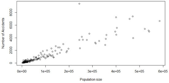
Figure 1. Scatterplot of the Model 1 data.

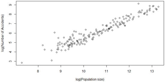
Figure 2. Scatterplot of the Model 1 data (on a natural log scale).

Table 2. Level of dependence between model variables.

Dataset/Model	${\mathit{X}}_1$	${\mathit{X}}_2$	Kendall’s $\mathit{\tau }$	Spearman’s $\mathit{\rho }$
AUS 1	ACC	Population	0.8123	0.9452
AUS 2	TPC	Population	0.8078	0.9479
AUS 3	K/I	Population	0.7981	0.9373
AUS 4	K/I	TPC	0.8372	0.9611
Swedish Motor	Policy Holder Years	Sum of Payments	0.7411	0.9030

Model 2 (AUS 2): In this model, we consider the two concomitant variables under study, namely the number of Third-Party Claims filed (TPC) and POP. TPC happens if a driver’s negligence results in the injury or death of another driver; the affected party or their family have the ability to file a claim against the guilty driver’s insurance company. We consider studying the dependence between TPC and the population of a given region in Australia because one would expect a larger volume of third-party claims to be filed in regions with higher populations. Needless to say, this is a good source of information for car insurance providers. From the scatterplot in Figure 3 and Figure 4, it appears that there exists a strong linear relationship between these two variables, which is also supported by the associated Kendall’s $\tau$ and Spearman’s $\rho$ values in Table 2 (Column 4, 5, Row 2).

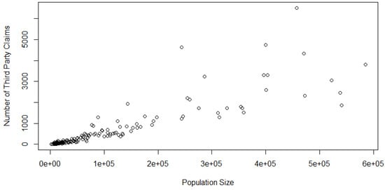
Figure 3. Scatterplot of the Model 2 data.

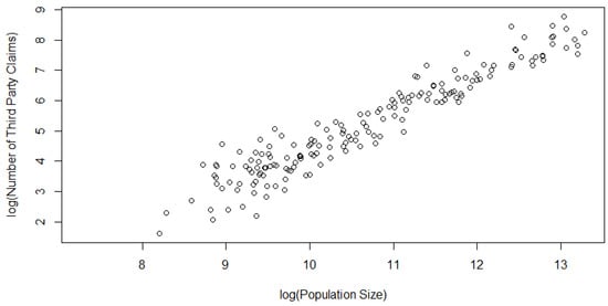
Figure 4. Scatterplot of the Model 2 data (on a natural log scale).

Model 3 (AUS 3): Next, we consider studying the dependence of a region’s population (POP) and the number of people killed or injured in an accident (K/I). Once we discovered that there was a strong dependence relationship between the number of third-party claims and the population size of a region, we realized that since third-party claims are a result of accidents with injuries involved, the number of people killed or injured could be greater in higher-populated areas where more third-party claims are filed. From the scatterplot in Figure 5 and Figure 6, it appears that there exists a strong linear relationship between these two variables, which is also supported by the associated Kendall’s $\tau$ and Spearman’s $\rho$ values in Table 2 (Column 4, 5, Row 3).

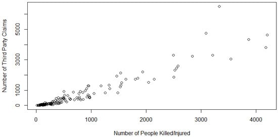
Figure 5. Scatterplot of the Model 4 data.

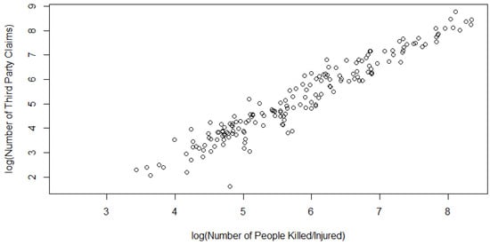
Figure 6. Scatterplot of the Model 4 data (on a natural log scale).

Model 4 (AUS 4): In this model, we consider studying the level of dependence between the number of people injured or killed in an automobile accident (K/I) and the corresponding number of third-party claims filed (TPC). As defined above in Model 2, third-party claims are filed in the event of an accident in which other drivers suffer injury from the negligence of another. While injury and death are not exclusive to the third party, we found a positive trend in the scatterplot of these two variables (Figure 7 and Figure 8). Hence, we chose to fit a copula to these two concomitant variables.

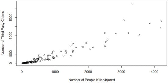
Figure 7. Scatterplot of the Model 4 data.

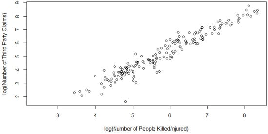
Figure 8. Scatterplot of the Model 4 data (on a natural log scale).

The non-exhaustive reasons for selecting four different models are as follows:

• For multicomponent insurance claim data, instead of a single representative value for the tail dependence measure, which would not reveal the partial dependence structure(s), it is better to observe the tail dependence structure pairwise. This way, one can eliminate to some extent the effect of lurking variable(s).
• Pairwise dependence measures help to identify (possibly one way or the other) which of the two components would be the most important to influence the associated portfolio risk.
• A class of bivariate copulas can be listed adequately for dealing with such types asymmetric insurance data, for example, where a specific class of extreme-value copulas or Archimedean copulas could be useful.

3.1.2. Dataset 2 (Swedish Motor Insurance Data)

This dataset represents the insurance information of 2182 motorists collected by the Swedish Committee on the Analysis of Risk Premium in 1977. It consists of the number of kilometers driven by a motorist (grouped into 5 categories), the geographical zone of a vehicle (grouped into 7 categories), the bonus variable (grouped into 7 categories), the make of the vehicle, the number of years that a motorist has been insured, the number of claims a motorist has filed, and the sum of the payments made by a motorist. We excluded the geographic zone and make of the vehicle variables from our consideration because while they are quantitatively defined, they describe qualitative variables and do not have a defined ordering. Due to the way the kilometers’ variable was defined, we were unable to come up with a model that showed a large amount of dependence, so the results of that model are excluded from this paper. Instead, we chose to study the dependence and subsequently search for the best possible bivariate copula model with the following variables of interest:

• $X_1$: Insured (number of years a motorist has been insured).
• $X_2$: Claims (sum of claim payments).

The scatterplots in Figure 9 and Figure 10 show a linear relationship between the variables.

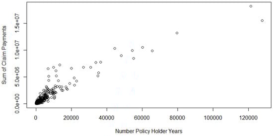
Figure 9. Scatterplot of the Swedish motor data.

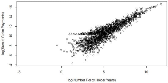
Figure 10. Scatterplot of the Swedish motor data (on a natural log scale).

The Table 2 and Table 3 below detail the results for each model. Note that all of these computations were performed in R.

Table 3. Model diagnostics and goodness of fit statistics.

Dataset/Model	Best-Fitted Copula	Parameter Estimates	AIC	BIC	Log Likelihood
AUS 1/Model 1	Frank	(18.42)	−377.38	−374.21	189.69
AUS 2/Model 2	Frank	(18.33)	−376.58	−373.41	189.29
AUS 3/Model 3	Tawn 1	(5.01, 0.95)	−373.11	−366.76	188.55
AUS 4/Model 4	Student t	(0.96, 4.61)	−442.33	−435.99	223.16
Swedish Motor	BB6	(1.59, 2.81)	−4095.96	−4084.58	2049.98

Table 2 outlines the level of concordance between each pair of variables in each model. When two variables are concordant, this means that higher values of one variable are associated with higher values of the other and vice versa for lower values. If these coefficients are closer to $0,$ this indicates low dependence or even independence. Conversely, if these coefficients are closer to $1,$ it tells us that the variables are dependent upon one another. From Table 2, we see that each pair of variables exhibits a strong level of dependence, since the concordance coefficients are close to $1.$ Table 3 represents various model diagnostics along with parameter estimates corresponding to the best-fitted bivariate copula. We expect the AIC and BIC to be minimal and the log likelihood to be maximal. Each copula shown in Table 3 represents the best fit for the pair of variables that were being tested according to the AIC, BIC, and log-likelihood criteria. The c.d.f. and p.d.f. plots corresponding to the best-fitted bivariate copulas listed in Table 3 are also provided in the Figure 11, Figure 12, Figure 13 and Figure 14.

Figure 11. Gaussian(0.8) c.d.f. and p.d.f.

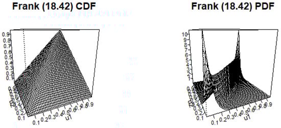
Figure 12. Frank c.d.f. and p.d.f. with $\alpha =18.42$.

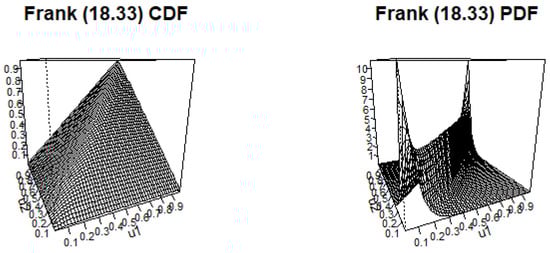
Figure 13. Frank c.d.f. and p.d.f. with $\alpha =18.33$.

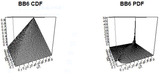
Figure 14. BB6 c.d.f. and p.d.f. with $\theta =1.59$ and $\delta =2.81$.

4. Structural Properties of the Fitted Bivariate Copula

This section presents the analysis of certain structural properties of the copulas. We begin our discussion with the Tawn type-1 copula.

4.1. Tawn Type-1 Copula

We can say the following regarding Tawn type-1 copula that was found to be the best-fitted bivariate copula for Model 3 from the dataset 1:

• The Tawn copula is a nonexchangeable extension of the Gumbel copula with three parameters (also known as the asymmetric logistic copula).
• Tawn copula’s definition is based around so-called Pickands dependence functions, see Franc et al. (2011) for pertinent details. Equation (4) in Franc et al. (2011) presents the way one can compute the density in the probability space using a Pickands function M:

  $$C\left(u,v\right)={\left(u,v\right)}^{A\left(w\right)},$$

  with $w=\frac{log\left(u\right)}{log\left(uv\right)}.$
• The Tawn copula’s Pickand function can be written as

  $$M\left(t\right)=\left(1-{\psi }_2\right)\left(1-t\right)+\left(1-{\psi }_1\right)t+{\left[{\left({\psi }_1(1-t)\right)}^{\theta }+{\left({\psi }_2\right)}^{\theta }\right]}^{1/\theta },$$

  with $t\in [0,1],0\le {\psi }_1,{\psi }_2\le 1$, and $\theta \in [1,\infty ).$ The Tawn copula is in actuality a Gumbel copula with two additional asymmetry parameters: ${\psi }_1$ and ${\psi }_2.$ If we set ${\psi }_1$ and ${\psi }_2$ equal to unity, the Gumbel copula is obtained. In the VineCopula package in $R,$ the Tawn type-1 copula refers to ${\psi }_1=1.$
• For this copula, the lower-tail dependent ${\lambda }_L=0.$ The corresponding upper-tail dependent ${\lambda }_U=0.8288,$ for the AUS3/Model 3 data for which Tawn type-1 copula appeared to be the best fit.

4.2. Frank Copula

The Frank copula (see, Nadarajah et al. 2017) has the following form:

$$C\left(u,v\right)={log}_{\alpha }\left[1+\frac{\left({\alpha }^u-1\right)\left({\alpha }^v-1\right)}{\alpha -1}\right],$$

for $\alpha >0.$ In this case, the positive dependence corresponds to $0<\alpha <1,$ independence corresponds to $\alpha \to 1,$ and negative dependence corresponds to $\alpha >1.$ Next, for this bivariate copula, we can write the following:

• The associated dual of the copula is denoted by $\tilde{C}\left(u,v\right)$ and is given by

  $$\tilde{C}\left(u,v\right)=u+v-C\left(u,v\right)=u+v-{log}_{\alpha }\left[1+\frac{\left({\alpha }^u-1\right)\left({\alpha }^v-1\right)}{\alpha -1}\right],$$
• Again, the associated co-copula denoted by $C^{*}\left(u,v\right)$ and is given by

  $$C^{*}\left(u,v\right)=1-C\left(1-u,1-v\right)=1-{log}_{\alpha }\left[1+\frac{\left({\alpha }^{1-u}-1\right)\left({\alpha }^{1-v}-1\right)}{\alpha -1}\right].$$

For the bivariate Frank copula, we have the following:

• The Kendall’s $\tau$ will be $\tau =4\left[\frac{3log\left(\alpha \right)(-2log(1-\alpha )+log\left(\alpha \right)+2)-6{\mathrm{Li}}_2\left(\alpha \right)+{\pi }^2}{6{log}^2\left(\alpha \right)}\right]-1,$ where ${\mathrm{Li}}_2\left(\alpha \right)$ is the PolyLog function (on using Mathematica).
• The Spearman’s $\rho$ will be

  $$\begin{array}{ccc}& & \rho =\hfill \\ & & {\int }_0^1\frac{v\left((1-\alpha )log(\alpha -1){\alpha }^v+(\alpha -1){\alpha }^{v}log\left((\alpha -1){\alpha }^v\right)-\alpha log\left(\alpha \right)\left({\alpha }^v-1\right)\right)}{log\left(\alpha \right)\left({\alpha }^v-1\right)\left({\alpha }^v-\alpha \right)}dv-3.\hfill \end{array}$$
• The Blomqvist’s $\beta$ expression will be

  $$\beta =4{log}_{\alpha }\left[1+\frac{{\left({\alpha }^{\frac{1}{2}-1}\right)}^2}{\alpha -1}\right].$$
  Tail dependence property of the bivariate Frank copula:
• For the upper-tail dependence (using L’Hôpital’s rule)

  $$\begin{array}{cc}\hfill {\lambda }_U& =\underset{u\uparrow 1}{lim}\frac{1-2u+{log}_{\alpha }\left[1+\frac{{({\alpha }^u-1)}^2}{\alpha -1}\right]}{1-u}\hfill \\ \hfill & \stackrel{H}{=}-\underset{u\uparrow 1}{lim}\left(-2+\left(\frac{1}{1+\frac{{({\alpha }^u-1)}^2}{\alpha -1}}\right)\left(\frac{2({\alpha }^u-1)({\alpha }^{u}log\alpha )}{(\alpha -1)log\alpha }\right)\right)\hfill \\ \hfill & =0.\hfill \end{array}$$
  Therefore, Frank’s copula is upper-tail dependent. Next, we determine if it is lower-tail dependent. Consider the limit

  $$\begin{array}{cc}\hfill {\lambda }_L& =\underset{u\downarrow 0}{lim}\frac{{log}_{\alpha }\left[1+\frac{{({\alpha }^u-1)}^2}{\alpha -1}\right]}{u}\hfill \\ \hfill & \stackrel{H}{=}\underset{u\downarrow 0}{lim}\frac{2({\alpha }^u-1)\left({\alpha }^u\right){(log\alpha )}^2}{1+\frac{{({\alpha }^u-1)}^2}{\alpha -1}}\hfill \\ \hfill & =0,\hfill \end{array}$$

  again, on using L’Hôpital’s rule. Consequently, the Frank copula is also lower-tail independent. Therefore, the bivariate Frank copula is asymptotically independent.

LTD and RTI property of the bivariate Frank copula:

Consider the following:

$$\frac{{\partial }^2}{\partial u^2}{C}_{\alpha }\left(u,v\right)=-\frac{log\left(\alpha \right){\alpha }^u\left({\alpha }^v-1\right)\left({\alpha }^v-\alpha \right)}{{\left(\alpha -{\alpha }^u+{\alpha }^{u+v}-{\alpha }^v\right)}^2}.$$

Therefore, $\frac{{\partial }^2}{\partial u^2}{C}_{\alpha }\left(u,v\right)\le 0$ for $0<\alpha <1;$ thus, $C_{\alpha }\left(u,v\right)$ is a concave function of u for $0<\alpha <1.$ It follows that if X and Y are continuous with the Frank family copula, then $SI\left(Y|X\right)$ (and by symmetry $SI\left(X|Y\right)$ as well). Again, from Theorem 5.2.12 (Nelsen (2006)) this implies the associated BB8 family copula also holds the LTD and RTI property, i.e., $LTD\left(Y|X\right)$ and $RTI\left(Y|X\right)$, and because of symmetry, $LTD\left(X|Y\right)$ and $RTI\left(X\right|Y).$

Furthermore, we see that both models are highly correlated in the center of their respective distributions. The Table 4 below summarizes the dependence structures discussed above and displays the generator function of this particular copula:

Table 4. Dependence of the Frank copula.

Generator Function	$\mathit{\varphi }\left(\mathit{t}\right)=-log\left(\frac{exp(-\mathit{\alpha }\mathit{t})-1}{exp(-\mathit{\alpha })-1}\right)$
Blomqvist $\beta$ (AUS 1)	0.9348
Blomqvist $\beta$ (AUS 2)	0.9329
Upper-Tail Dependence	0
Lower-Tail Dependence	0
Kendall’s $\tau$	given earlier

4.3. Bivariate t Copula

The t copula (see Embrechts et al. (2001) or Fang and Fang (2002) and the references cited therein) can be thought of as representing the dependence structure implicit in a multivariate t distribution. The two-dimensional unique t copula associated with a bivariate random vector $Y={\left(Y_1,Y_2\right)}^T,$ is given by

$$C_{\delta }^t\left(u,v\right)={\int }_{-\infty }^{t_{\delta }^{-1}\left(u\right)}{\int }_{-\infty }^{t_{\delta }^{-1}\left(v\right)}\frac{\mathsf{\Gamma }\left((\delta +2)/2\right)}{\mathsf{\Gamma }\left(\delta /2\right)\sqrt{\{}{\left(\pi \delta \right)}^2\left|\mathsf{\Sigma }\right|\}}{\left[1+\frac{y^T{\mathsf{\Sigma }}^{-1}y}{\delta }\right]}^{-\frac{\delta +2}{2}}d{y}_{1}d{y}_2,$$

where $t_{\delta }^{-1}(.)$ denotes the quantile function of a standard univariate $t_{\delta }(.)$ distribution. Furthermore, $\mathsf{\Sigma }$ is the correlation matrix given by

$$\mathsf{\Sigma }=\left[\begin{array}{cc}1& \rho \\ \rho & 1\end{array}\right],$$

where $\rho$ is the correlation coefficient between $Y_1,$ and $Y_2.$ The determinant of this matrix, denoted by $\left|\mathsf{\Sigma }\right|$, is given by $\left|\mathsf{\Sigma }\right|=1-{\rho }^2.$ Next, one may verify the following regarding the dependence structure for a bivariate t copula

• Kendall’s $\tau$ will be

  $$\tau =\frac{2}{\pi }arcsin\rho ,$$

  for the proof, see Fang and Fang (2002).
• The tail dependence coefficient (associated with a bivariate t copula as given earlier) $\lambda$ is given by

  $$\lambda =2t_{\delta +1}\left(-\frac{\sqrt{\{}\delta +1\}\sqrt{\{}1-\rho \}}{\sqrt{\{}1+\rho \}}\right),$$

  where $t_{\delta +1}$ is the univariate central student t distribution with $(\delta +1)$ degrees of freedom and $\rho$ is the correlation coefficient. It is important to note that a student t-copula may exhibit both the positive and negative tail dependence, although the “overall” association is negative $\rho <0$. Furthermore, a student t-copula with a large value of $\delta$ tends to have a 0 tail dependence even though the correlation is 0. The t-copula can capture the asymptotic dependence even when the variables are negatively (inversely) associated (see, Embrechts et al. 2001). In the t-copula formula, as  $\delta$ increases, the tail dependence weakens, and thus, the probability of occurrence of extreme values reduces.
  For illustrative purposes, we provide the following picture in Figure 15 (generated through the https://copulatheque.shinyapps.io/copulas/ (accessed on 15 June 2022) created by BenGraeler) showing a student t-copula with $\rho =-0.3$ and $\delta =1$, which gives the value of Kendall’s $\tau =-0.19$ and upper- and lower-tail dependence of $\lambda =0.19$.
  

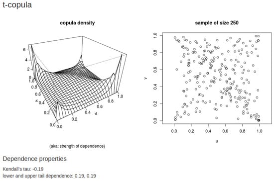  Figure 15. Student t− copula density with $\delta =2$ and with Kendall’s $\tau =-0.19$.
  The estimation of a student t-copula is quite difficult. Noticeably, the marginal tails (for bivariate and/or multivariate data distributions) of financial data are usually heavy tailed, and hence this should be fitted by a t-distribution and not by a Gaussian distribution. In addition, the dependence in joint extremes of bivariate and/or multivariate financial data suggests a dependence structure allowing for tail dependence. Consequently, the use of t-copulas has become popular for modeling dependencies in financial data. Some recent applications have been: analysis of nonlinear and asymmetric dependence in the German equity market Sun et al. (2008); estimation of large portfolio loss probabilities Chan and Kroese (2010); and risk modeling for future cash flow Pettere and Kollo (2011). See also Dakovic and Czado (2011).
  One may subsequently obtain the expressions for the upper-tail as well as lower-tail dependence from the above. For details, see (Demarta and McNeil 2005, p. 4, Proposition 1).

4.4. BB6 (Joe–Gumbel) Copula

The BB6 copula (see Joe 1997) has the following form:

$$\begin{array}{cc}\hfill C(u,v)& =1-(1-exp(-{[{(-log(1-{\overline{u}}^{\theta }))}^{\delta }+{(-log(1-{\overline{v}}^{\theta }))}^{\delta }]}^{\frac{1}{\delta }}){)}^{\frac{1}{\theta }},u\ge 0,v\le 1,\theta \ge 1,\delta \ge 1.\hfill \end{array}$$

where $\overline{u}=1-u$ and $\overline{v}=1-v$.

Tail dependence property of the bivariate BB6 copula

The lower-tail and upper-tail dependence coefficients can be calculated using the same methodology that we used for the Frank copula. For the upper-tail dependence coefficient, we obtain the following:

$$\begin{array}{cc}\hfill {\lambda }_U& =\underset{u\uparrow 1}{lim}\frac{1-2u+1-(1-exp(-[2{(-log(1-{\overline{u}}^{\theta }))}^{\delta }]){)}^{\frac{1}{\theta }}}{1-u}\hfill \\ \hfill & \stackrel{H}{=}\underset{u\uparrow 1}{lim}2-2^{\frac{1}{\delta }}{(1-u)}^{\theta -1}exp[2^{\frac{1}{\delta }}log(1-{(1-u)}^{\theta })]{(1-exp[2^{\frac{1}{\delta }}log(1-{(1-u)}^{\delta }])}^{\frac{1}{\theta }-1}=2-2^{\frac{1}{\theta \delta }}.\hfill \end{array}$$

Similarly, for the lower-tail dependence coefficient:

$$\begin{array}{cc}\hfill {\lambda }_L& =\underset{u\downarrow 0}{lim}\frac{1-(1-exp(-[2{(-log(1-{\overline{u}}^{\theta }))}^{\delta }]){)}^{\frac{1}{\theta }}}{u}\hfill \\ \hfill & \stackrel{H}{=}\underset{u\downarrow 0}{lim}{2}^{\frac{1}{\delta }}{(1-u)}^{\theta -1}exp[2^{\frac{1}{\delta }}log(1-{(1-u)}^{\theta })]{(1-exp[2^{\frac{1}{\delta }}log(1-{(1-u)}^{\delta }])}^{\frac{1}{\theta }-1}=0.\hfill \end{array}$$

Therefore, the BB6 copula is not asymptotically independent. However, from the given expression for ${\lambda }_U,$ it is quite clear that as both $\theta$ and $\delta$ are close to $1,$ ${\lambda }_U$ is close to zero. This would imply that the BB6 copula is asymptotically independent in such a case. Furthermore, from the expression for ${\lambda }_U$, it appears that as the values of $\delta$ and $\theta$ increases, the value of ${\lambda }_U$ increases. This implies the fact that this copula might not be that useful to model the dependence structure for financial data in general, as such tend to exhibit tail dependence, especially lower-tail dependence. However, if the data suggests that the estimated values of the parameters $\delta$ and $\theta$ are larger than one, then it may be utilized to model financial data, such as insurance data that exhibit some amount of tail dependence.

LTD and RTI property of the bivariate Frank copula:

Consider the following:

$$\begin{array}{cc}\hfill & \frac{{\partial }^2}{\partial u^2}{C}_{\theta ,\delta }(u,v)\hfill \\ \hfill & ={\left[{\left({(1-u)}^{\theta }-1\right)}^2{\left(exp\left({\left({\left(-log\left(1-{(1-u)}^{\theta }\right)\right)}^{\delta }+{\left(-log\left(1-{(1-v)}^{\theta }\right)\right)}^{\delta }\right)}^{\frac{1}{\delta }}\right)-1\right)}^2\right]}^{-1}\hfill \\ \hfill & \times \left[A_1\times A_2\left\{A_3+{\left(1-u\right)}^{\theta }\times \left(B_1+B_2+B_3\right)\right\}\right],\hfill \end{array}$$

where

$$\begin{array}{cc}\hfill A_1& ={\left(1-u\right)}^{\theta -2}{\left(-log\left(1-{(1-u)}^{\theta }\right)\right)}^{\delta -2}\hfill \\ \hfill & \times {\left[1-exp\left(-{\left({\left(-log\left(1-{(1-u)}^{\theta }\right)\right)}^{\delta }+{\left(-log\left(1-{(1-v)}^{\theta }\right)\right)}^{\delta }\right)}^{\frac{1}{\delta }}\right)\right]}^{\frac{1}{\theta }},\hfill \end{array}$$

$$A_2={\left[{\left(-log\left(1-{(1-u)}^{\theta }\right)\right)}^{\delta }+{\left(-log\left(1-{(1-v)}^{\theta }\right)\right)}^{\delta }\right]}^{\frac{1}{\delta }-2},$$

$$\begin{array}{cc}\hfill A_3& =\left(\theta +{(1-u)}^{\theta }-1\right)log\left(1-{(1-u)}^{\theta }\right)\left({\left(-log\left(1-{(1-u)}^{\theta }\right)\right)}^{\delta }+{\left(-log\left(1-{(1-v)}^{\theta }\right)\right)}^{\delta }\right)\hfill \\ \hfill & \times \left[exp\left({\left({\left(-log\left(1-{(1-u)}^{\theta }\right)\right)}^{\delta }+{\left(-log\left(1-{(1-v)}^{\theta }\right)\right)}^{\delta }\right)}^{\frac{1}{\delta }}\right)-1\right],\hfill \end{array}$$

$$B_1=-{\left(-log\left(1-{(1-u)}^{\theta }\right)\right)}^{\delta }{\left({\left(-log\left(1-{(1-u)}^{\theta }\right)\right)}^{\delta }+{\left(-log\left(1-{(1-v)}^{\theta }\right)\right)}^{\delta }\right)}^{\frac{1}{\delta }},$$

$$\begin{array}{cc}\hfill B_2& =\theta \left[{\left(-log\left(1-{(1-u)}^{\theta }\right)\right)}^{\delta }{\left({\left(-log\left(1-{(1-u)}^{\theta }\right)\right)}^{\delta }+{\left(-log\left(1-{(1-v)}^{\theta }\right)\right)}^{\delta }\right)}^{\frac{1}{\delta }}\right.\hfill \\ \hfill & \left.-\delta {\left(-log\left(1-{(1-v)}^{\theta }\right)\right)}^{\delta }+{\left(-log\left(1-{(1-v)}^{\theta }\right)\right)}^{\delta }\right]\hfill \\ \hfill & \times exp\left({\left({\left(-log\left(1-{(1-u)}^{\theta }\right)\right)}^{\delta }+{\left(-log\left(1-{(1-v)}^{\theta }\right)\right)}^{\delta }\right)}^{\frac{1}{\delta }}\right),\hfill \end{array}$$

$$B_3=\left(\delta -1\right)\theta {\left(-log\left(1-{(1-v)}^{\theta }\right)\right)}^{\delta }.$$

Therefore, $\frac{{\partial }^2}{\partial u^2}{C}_{\theta ,\delta }(u,v)\le 0$ for $\theta >1$ and for any $\delta \ge 1;$ thus, $C_{\theta ,\delta }(u,v)$ is a concave function of u for $\theta >1$ and for any $\delta \ge 1.$ It follows that if X and Y are continuous with the BB6 family copula, then $SI\left(Y\right|X)$ (and by symmetry $SI\left(X\right|Y)$ as well). Again, from Theorem 5.2.12 (Nelsen 2006, p. 197) this implies the associated BB8 family copula also holds the LTD and RTI property, i.e., $LTD\left(Y\right|X)$ and $RTI\left(Y\right|X)$ and because of symmetry $LTD\left(X\right|Y)$ and $RTI\left(X\right|Y).$ Note that for $0<\theta \le 1$, it is inconclusive for this copula family. In Table 5, below, we provide the the summary of the dependence measures for the BB6 copula for the Swedish motor insurance data.

Table 5. Dependence structures of the BB6 copula for the Swedish motor insurance data.

Generator Function	$\mathit{\varphi }\left(\mathit{t}\right)={(-log[1-{(1-\mathit{t})}^{\mathit{\theta }}])}^{\mathit{\delta }}$
Blomqvist Beta (General)	$\beta =4\left(1-{\left(1-e^{-{[{(-log(1-{\frac{1}{2}}^{\theta }))}^{\delta }+{(-log(1-{\frac{1}{2}}^{\theta }))}^{\delta }]}^{\frac{1}{\delta }}}\right)}^{\frac{1}{\theta }}\right)$
Blomqvist $\beta$ (Swedish Auto)	0.7397
Upper-Tail (Swedish Auto)	$2-2^{\frac{1}{\delta \theta }}=0.8321$
Lower-Tail Dependence	0
Kendall’s $\tau$	$1+\frac{4}{\delta \theta }{\int }_0^1(-log(1-{(1-t)}^{\theta })(1-t)(1-{(1-t)}^{-\theta })dt$

5. Concluding Discussion and Remarks

In this article, we considered several well-known bivariate copulas, including the Tawn type-1, Frank, and BB6 families of copula based on the R package VineCopula for fitting two well-known insurance datasets arising out of automobile insurance. In addition, we also provided several useful structural properties of the selected bivariate copulas such as the LTD and RTI property, primarily focusing on the tail dependence properties, which are very important for studying dependence for insurance claims. This study shows that certain types of Archimedean copula with heavy tail dependence property are a reasonable framework to start with in terms of modeling insurance claim data, both in the bivariate as well as in the case of multivariate domains as appropriate. The goodness-of-fit statistics are provided in terms of AIC and BIC values as well as the log-likelihood values. As  future research, we will be focusing on datasets from other domains (such as health care data), and  we will consider the fitting to a trivariate and in higher dimensions as well based on the vine copula methodology. We will report our findings in a separate article. The tail-dependence coefficient has several applications, including: validation and verification of weather and climate models in reproducing extreme events; analysis of simultaneous extremes; probabilistic assessment of occurrences of extremes; and understanding climate variability. For example, by deriving tail-dependence coefficients for simulations of a numerical weather prediction model or a climate model, one can evaluate whether these models produces dependencies as seen in the observations. These approaches are not limited to precipitation, they also include a wide variety of earth science variables. This study of extreme tail dependence on local, regional, and global scales can assist in planning and policy making as well as validating numerical models, thus providing a valuable tool for understanding how extreme events impact society. For future policy implementation out of this study, one may mention the following:

• Classes of extreme values of copulas (such as Tawn type-1, Frank, and BB6) are useful in modeling dependence for insurance claim data from the automobile industry that are asymmetric in nature.
• All the fitted bivariate copulas have one property in common, which is the nonzero value of the upper-tail dependence measure. This implies the fact that one observes an extremely large value for one component together with an extremely large value for the other component, a feature which is expected for insurance claim dataset-generated dependence structure. As a consequence, one can start with bivariate and multivariate copulas (as the case may be) that have a nonzero value of the upper-tail dependence measure ${\lambda }_U$ when examining the dependence structure related to insurance claim data from the automobile industry.
• As a future study, it will be interesting to see whether such a class of extreme value copulas can be useful for insurance claims from other industries. Furthermore, for portfolio risk assessment, the effectiveness of such classes of copulas would be the subject matter of future research.

References

- Alexeev, Vitali, Katja Ignatieva, and Thusitha Liyanage. 2021. Dependence Modelling in Insurance via Copulas with Skewed Generalised Hyperbolic Marginals. Studies in Nonlinear Dynamics and Econometrics 25: 2. [Google Scholar] [CrossRef]
- Blomqvist, Nils. 1950. On a measure of dependence between two random variables. Annals of Mathematical Statistics 21: 593–600. [Google Scholar] [CrossRef]
- Chan, Joshua C. C., and Dirk P. Kroese. 2010. Efficient estimation of large portfolio loss probabilities in t-copula models. European Journal of Operational Research 205: 361–67. [Google Scholar] [CrossRef] [Green Version]
- Dakovic, Rada, and Claudia Czado. 2011. Comparing point and interval estimates in the bivariate t-copula model with application to financial data. Statistical Papers 52: 709–31. [Google Scholar] [CrossRef]
- Demarta, Stefano, and Alexander J. McNeil. 2005. The t Copula and Related Copulas. International Statistical Review 73: 111–29. [Google Scholar] [CrossRef]
- Embrechts, Paul, Alexander McNeil, and Daniel Straumann. 2001. Correlation and dependency in risk management: Properties and pitfalls. In Risk Management: Value at Risk and Beyond. Cambridge, UK: Cambridge University Press, pp. 176–223. Available online: http://www.math.ethz.ch/~mcneil (accessed on 15 June 2022).
- Fang, Hong-Bin, Kai-Tai Fang, and Samuel Kotz. 2002. The meta elliptical distributions with given marginals. Journal of Multivariate Analysis 82: 1–16. [Google Scholar] [CrossRef] [Green Version]
- Franc, Jean-Pierre, Michel Riondet, Ayat Karimi, and Georges L. Chahine. 2011. Impact load measurements in an erosive cavitating flow. Journal of Fluids Engineering 133: 121301. [Google Scholar] [CrossRef]
- Joe, Harry. 1997. Multivariate Models and Dependence Concepts. New York: Chapman & Hall. [Google Scholar]
- Mensi, Walid, Aviral Tiwari, Elie Bouri, David Roubaud, and Khamis H. Al-Yahyaee. 2017. The dependence structure across oil, wheat, and corn: A wavelet-based copula approach using implied volatility indexes. Energy Economics 66: 122–39. [Google Scholar] [CrossRef]
- Nadarajah, Saralees, Afuecheta Emanuel, and Chan Stephen. 2017. A compendium of copulas. Statistica 77: 279–328. [Google Scholar]
- Naeem, Muhammad Abubakr, Elie Bouri, Mabel D. Costa, Nader Naifar, and Syed Jawad Hussain Shahzad. 2021. Energy markets and green bonds: A tail dependence analysis with time-varying optimal copulas and portfolio implications. Resources Policy 74: 102418. [Google Scholar] [CrossRef]
- Nelsen, Roger B. 1999. An Introduction to Copulas, 1st ed. New York: Springer. [Google Scholar]
- Nelsen, Roger B. 2006. An Introduction to Copulas, 2nd ed. New York: Springer. [Google Scholar]
- Pettere, Gaida, and Tõnu Kollo. 2011. Risk modeling for future cash flow using skew t-copula. Communications in Statistics-Theory and Methods 40: 2919–25. [Google Scholar] [CrossRef]
- Pfeifer, Dietmar, and Johana Nešlehová. 2003. Modeling dependence in finance and insurance: The copula approach. Blätter der DGVFM 26: 177–91. [Google Scholar] [CrossRef]
- Shi, Peng, Xiaoping Feng, and Jean-Philippe Boucher. 2016. Multilevel modeling of insurance claims using copulas. The Annals of Applied Statistics 10: 834–63. [Google Scholar] [CrossRef]
- Sklar, Abe. 1959. Fonctions de rpartition à n dimensions et leurs marges. Publications de l’Institut Statistique de l’Université de Paris 8: 229–231. [Google Scholar]
- Sklar, Abe. 1973. Random variables, joint distribution functions, and copulas. Kybernetika (Prague) 9: 449–60. [Google Scholar]
- Sun, Wei, Svetlozar Rachev, Stoyan V. Stoyanov, and Frank J. Fabozzi. 2008. Multivariate skewed Student’s t copula in the analysis of nonlinear and asymmetric dependence in the German equity market. Studies in Nonlinear Dynamics & Econometrics 12: 1–37. [Google Scholar]
Publisher’s Note: MDPI stays neutral with regard to jurisdictional claims in published maps and institutional affiliations. |
© 2022 by the authors. Licensee MDPI, Basel, Switzerland. This article is an open access article distributed under the terms and conditions of the Creative Commons Attribution (CC BY) license (https://creativecommons.org/licenses/by/4.0/).