Portfolio Optimization Constrained by Performance Attribution

Abstract

This paper investigates performance attribution measures as a basis for constraining portfolio optimization. We employ optimizations that minimize conditional value-at-risk and investigate two performance attributes, asset allocation (AA) and the selection effect (SE), as constraints on asset weights. The test portfolio consists of stocks from the Dow Jones Industrial Average index. Values for the performance attributes are established relative to two benchmarks, equi-weighted and price-weighted portfolios of the same stocks. Performance of the optimized portfolios is judged using comparisons of cumulative price and the risk-measures: maximum drawdown, Sharpe ratio, Sortino–Satchell ratio and Rachev ratio. The results suggest that achieving SE performance thresholds requires larger turnover values than that required for achieving comparable AA thresholds. The results also suggest a positive role in price and risk-measure performance for the imposition of constraints on AA and SE.

1. Introduction

How well a portfolio performs is always the major concern for investors, and is usually the major metric reflecting investor confidence in the portfolio’s management. In common terms, a good portfolio delivers satisfactory return with low risk. Attribution analysis provides measures for how well an portfolio is being managed. Paraphrasing from Bacon (2008), performance attribution is a technique used to quantify the excess return (relative to a benchmark) of a portfolio and explain that performance in terms of investment strategy and market conditions. From a management perspective, attribution analysis has been used to monitor performance, to identify early indications of underperformance, and gain investor confidence by demonstrating a thorough understanding of the performance drivers. As far as we are aware, performance attribution measures are currently used exclusively as a diagnostic, in the sense that if today’s attribute values underperform, then changes are implemented in the portfolio with the goal of improving tomorrow’s attribute values. In this work, we investigate the imposition of performance attribute constraints to guarantee that tomorrow’s portfolio achieves the required attribute values.

Following the fundamental work on performance attribution by Brinson and Fachler (1985) and Brinson et al. (1986), we decompose excess return into two quantities that reflect investment strategy: asset allocation (AA), which measures the contribution of each asset class in a portfolio to total performance of the portfolio, and the selection effect (SE), which measures the impact of choice of assets within each class in the portfolio. As is apparent from their definitions in the next section, AA and SE measure the differences between mean performance of asset classes in a managed portfolio and those of a market benchmark, and are therefore ‘blind’ to volatility effects, i.e., to tail-risk. Motivated by this and by the work of Biglova and Rachev (2007) and Rachev et al. (2009), we investigate the impact on portfolio optimization using AA and SE as additional constraints on asset weights as a method of combining performance and tail-risk control. We apply this methodology to a test portfolio of stocks comprising a major market index; specifically the Dow Jones Industrial Average. Optimization is performed by minimizing conditional value-at-risk (CVaR) at a specified quantile level, $\alpha$. For the required market benchmark we consider two options, an equi-weighted portfolio and a price-weighted portfolio, comprised of the same assets. Performance of the resulting optimal portfolios is measured in terms of cumulative portfolio price and standard risk-measures.

Section 2 of the paper discusses performance attribution, the constrained CVaR portfolio optimizations and the risk-measures employed to gauge their performance. Section 3 presents the results of the methodology applied to the test portfolio. Section 4 summarizes our conclusions.

2. Description of the Approach

Consider a managed portfolio p comprised of N assets, consisting of M asset classes with $n_i$ assets in class $i;i=1,\dots ,M$, such that ${\sum }_{i=1}^M{n}_i=N$. Let b denote a benchmark portfolio composed of Q assets comprising the same M asset classes, with $q_i$ assets in class $i;i=1,\dots ,M$, such that ${\sum }_{i=1}^M{q}_i=Q$. Let the index pair, $ij;i=1,\dots ,M;j=1,\dots ,n_i$, identify portfolio asset j in class i, with the analogous identification for benchmark assets. Denote the daily closing price of an asset as $S_{ij}\left(t\right)$ and its corresponding log-return as $r_{ij}\left(t\right)=ln\left(S_{ij}\left(t\right)/S_{ij}(t-1)\right)$. For brevity, we will suppress the time variable for most of the discussion in this section. Let $w_{ij}^{\left(p\right)}$ denote the weight of asset $ij$ in portfolio p, and $w_{ij}^{\left(b\right)}$ denote asset weight in the benchmark. We assume all weights are non-negative; that is, all portfolios considered take long-only positions. Let $w_i^{\left(p\right)}={\sum }_{j=1}^{n_i}{w}_{ij}^{\left(p\right)}$ and $w_i^{\left(b\right)}={\sum }_{j=1}^{q_i}{w}_{ij}^{\left(b\right)}$ represent the total weights of the assets in class i in the portfolio and benchmark respectively. Note that for any portfolio fully invested in its component assets (which we assume is the case in this study), ${\sum }_{i=1}^M{w}_i^{\left(p\right)}={\sum }_{i=1}^M{w}_i^{\left(b\right)}=1$.

The quantities AA and SE for asset class i are defined as follows (Biglova and Rachev 2007): 1

$$\begin{array}{cc}\hfill {\mathrm{AA}}_i& =\left(w_i^{\left(p\right)}-w_i^{\left(b\right)}\right)\left(R_i^{\left(b\right)}-R^{\left(b\right)}\right),\hfill \end{array}$$

(1)

$$\begin{array}{cc}\hfill {\mathrm{SE}}_i& =w_i^{\left(b\right)}\left(R_i^{\left(p\right)}-R_i^{\left(b\right)}\right),\hfill \end{array}$$

(2)

where

$$R_i^{\left(p\right)}=\sum _{j=1}^{n_i}\frac{w_{ij}^{\left(p\right)}}{w_i^{\left(p\right)}}\mathbb{E}\left[r_{ij}\right],R_i^{\left(b\right)}=\sum _{j=1}^{q_i}\frac{w_{ij}^{\left(b\right)}}{w_i^{\left(b\right)}}\mathbb{E}\left[r_{ij}\right],R^{\left(b\right)}=\sum _{i=1}^M\sum _{j=1}^{q_i}{w}_{ij}^{\left(b\right)}\mathbb{E}\left[r_{ij}\right],$$

(3)

and $\mathbb{E}\left[·\right]$ denotes expected value. In (3), the ratio $w_{ij}^{\left(p\right)}/w_i^{\left(p\right)}$ represents the fractional weight held by asset j in class i in portfolio p. (That is ${\sum }_{j=1}^{n_i}\left(w_{ij}^{\left(p\right)}/w_i^{\left(p\right)}\right)=1$.) Thus $R_i^{\left(p\right)}$ (similarly $R_i^{\left(b\right)}$) represents an expected log-return for asset class i considered as a fully-invested portfolio by itself. In contrast, $R^{\left(b\right)}$ represents the usual expected log-return for the entire benchmark portfolio.2 From (3) we have $R^{\left(b\right)}={\sum }_{i=1}^M{w}_i^{\left(b\right)}{R}_i^{\left(b\right)}$. Similarly we have the usual expected log-return for portfolio p,

$$R^{\left(p\right)}=\sum _{i=1}^M\sum _{j=1}^{n_i}{w}_{ij}^{\left(p\right)}\mathbb{E}\left[r_{ij}\right]=\sum _{i=1}^M{w}_i^{\left(p\right)}{R}_i^{\left(p\right)}.$$

(4)

The excess return, $S=R^{\left(p\right)}-R^{\left(b\right)}$, can be viewed as the value added by portfolio management. From (1) through (4),

$$S=\sum _{i=1}^M\left({\mathrm{AA}}_i+{\mathrm{SE}}_i+{\mathrm{I}}_i\right)=\mathrm{AA}+\mathrm{SE}+\mathrm{I},$$

(5)

where ${\mathrm{I}}_i=\left(w_i^{\left(p\right)}-w_i^{\left(b\right)}\right)\left(R_i^{\left(p\right)}-R_i^{\left(b\right)}\right)$ is an “interaction” term. AA, SE and I are, respectively, the total asset allocation, total selection effect, and total interaction terms for portfolio p. The contribution to the total value added to the excess return, S, from asset class i is ${\mathrm{AA}}_i$, while ${\mathrm{SE}}_i$ represents the contribution to S determined by the choice of assets within class i. To understand these interpretations, consider first the sign of the value of ${\mathrm{AA}}_i$ in (1).

• If $R_i^{\left(b\right)}-R^{\left(b\right)}>0$, the expected return from asset class i in the benchmark is outperforming the total expected return for the benchmark. Therefore if $w_i^{\left(p\right)}-w_i^{\left(b\right)}>0$, the weight of asset class i in portfolio p is larger than in the benchmark, capitalizing further on the better return from class i. Otherwise, if $w_i^{\left(p\right)}-w_i^{\left(b\right)}<0$, the class i weighting in portfolio p is hurting the potential performance of that class (as determined by the benchmark).
• If $R_i^{\left(b\right)}-R^{\left(b\right)}<0$, the expected return from asset class i in the benchmark is under-performing the total expected return for the benchmark. Therefore if $w_i^{\left(p\right)}-w_i^{\left(b\right)}<0$, the weight of asset class i in portfolio p is smaller than in the benchmark, further suppressing the poorer return from that class. Otherwise, if $w_i^{\left(p\right)}-w_i^{\left(b\right)}>0$, the class i weighting in portfolio p is overweighting the poor performance of that class.

Thus, a positive sign for the value of ${\mathrm{AA}}_i$ indicates a “correct” decision in the management of portfolio p relative to the benchmark while a negative sign indicates a “poor” decision. The magnitude of ${\mathrm{AA}}_i$ quantifies how good or poor the decision is.

Similarly, as we assume3 $w_i^{\left(b\right)}>0;i=1,\dots ,M$, a positive sign for the value of ${\mathrm{SE}}_i$ in (2) indicates that the expected return from the choice of assets in class i in portfolio p is outperforming that class in the benchmark, while a negative sign indicates that the expected return from the choice of assets in class i in portfolio p is under-performing.

The interaction term, ${\mathrm{I}}_i$, captures the part of the excess return unexplained by asset allocation and selection effect. Written as

$${\mathrm{I}}_i=\frac{{\mathrm{AA}}_i{\mathrm{SE}}_i}{w_i^{\left(b\right)}\left(R_i^{\left(b\right)}-R^{\left(b\right)}\right)},$$

(6)

it can be viewed as the product of the asset allocation and selection effect contributions of class i to portfolio p compared to the weighted excess return of class i in the benchmark b. Alternatively, written as

$${\mathrm{I}}_i=\left(\frac{w_i^{\left(p\right)}}{w_i^{\left(b\right)}}-1\right){\mathrm{SE}}_i,$$

(7)

it can be interpreted as the product of the asset selection effect and the over- or under-weighted part of asset class i. The relationship (7) between ${\mathrm{I}}_i$ and ${\mathrm{SE}}_i$ reveals a simple form for the sum of the selection effect and interaction terms,

$${\overline{\mathrm{SE}}}_i:={\mathrm{SE}}_i+{\mathrm{I}}_i=w_i^{\left(p\right)}\left(R_i^{\left(p\right)}-R_i^{\left(b\right)}\right).$$

(8)

Equation (8) provides a way to incorporate a constraint on the sum of the selection and interaction effects for class i; however, we will not consider such a combined constraint in this study.

Portfolio optimizations that maximize return while minimizing risk (subject to additional constraints) require specification of a proxy measure for risk. Common examples of risk proxy include: the variance of the portfolio (Markowitz 1952); value-at-risk (VaR) (JP Morgan 1996); expected tail loss (ETL); conditional value-at-risk (CVaR) (Rockafellar and Uryasev 2000);4 and mean absolute-deviation (Konno and Yamazaki 1991). Measures, such as VaR and CVaR, that focus on tail-risk became very popular as the result of the need to understand exposure to loss under ‘extreme’ market events. (See Gava et al. (2021) for a recent study demonstrating that consideration of tail risk can successfully reduce sharp losses in multi-asset portfolios). However VaR has undesirable mathematical characteristics; except when the underlying random process is Gaussian, VaR is not a coherent risk measure as it lacks the properties of subadditivity and convexity (Artzner et al. 1999). As a risk measure, CVaR is coherent (Pflug 2000); its use as a standard has grown to the point that the Basel III regulatory framework for banks requires it. We therefore use CVaR as the risk measure for our portfolio optimizations.

The random return Y of a portfolio is expressed as realizations, y, of a profit(+) - loss(−) function $f(\mathit{w},\mathit{r})$ of the (column vectors of) asset weights $\mathit{w}$ and returns $\mathit{r}$. Let $p\left(\mathit{r}\right)$ denote the probability density function determining the daily asset returns $\mathit{r}$. For any fixed value of $\mathit{w}$, the cumulative distribution of the daily portfolio return is given by

$$P(\mathit{w},Y\le y)\equiv F(\mathit{w},y)={\int }_{f(\mathit{w},\mathit{r})\le y}p\left(\mathit{r}\right)d\mathit{r}.$$

(9)

The value-at-risk is5

$${\mathrm{VaR}}_{\alpha }\left(\mathit{w}\right)=inf\left\{y\in \mathbb{R}\mid F(\mathit{w},y)\ge \alpha \right\},$$

(10)

where $\alpha \in (0,1)$ is a prescribed tail risk probability; equivalently $1-\alpha$ is a prescribed quantile level, typically having value of $1-\alpha =0.95,0.99$ or $0.995$. Assuming $F(\mathit{w},y)$ is continuous, conditional value-at-risk can be expressed as6

$${\mathrm{CVaR}}_{\alpha }\left(\mathit{w}\right)=\frac{1}{\alpha }{\int }_{f(\mathit{w},\mathit{r})\le {\mathrm{VaR}}_{\alpha }\left(\mathit{w}\right)}f(\mathit{w},\mathit{r})p\left(\mathit{r}\right)d\mathit{r}.$$

(11)

Rockafellar and Uryasev (2000) show that the function7

$$F_{\alpha }(\mathit{w},\gamma )=\gamma -\frac{1}{\alpha }{\int }_{{\mathbb{R}}^n}{\left(\gamma -f(\mathit{w},\mathit{r})\right)}^{+}p\left(\mathit{r}\right)d\mathit{r},$$

(12)

where ${\left(x\right)}^{+}=\max (x,0)$, has the following properties: (1) for fixed $\mathit{w}$, $\gamma ={\mathrm{VaR}}_{\alpha }\left(\mathit{w}\right)$ minimizes $F_{\alpha }(\mathit{w},\gamma )$; (2) $F_{\alpha }(\mathit{w},{\mathrm{VaR}}_{\alpha }\left(\mathit{w}\right))={\mathrm{CVaR}}_{\alpha }\left(\mathit{w}\right)$; and (3) $F_{\alpha }(\mathit{w},\gamma )$ is convex in $\gamma$ (and convex with respect to $(\mathit{w},\gamma )$ if $f(\mathit{w},\mathit{r})$ is convex in $\mathit{w}$).

When evaluated for a portfolio consisting of a finite sample of asset returns, $\mathit{r}\left(t\right),t=1,$ …, T with $f(\mathit{w},\mathit{r})={\mathit{w}}^{\prime }\mathit{r}$, the discrete form of (12) results in the following minimization problem,

$$\underset{\mathit{w}}{min}{\mathrm{CVaR}}_{\alpha }\left(\mathit{w}\right)=\underset{\mathit{w},\gamma }{min}\left\{\gamma -\frac{1}{\alpha T}\sum _{t=1}^T{\left(\gamma -{\mathit{w}}^{\prime }\mathit{r}\left(t\right)\right)}^{+}\right\}.$$

(13)

The approach by Rockafellar and Uryasev proceeds by converting (13) to a linear objective function by introducing the variable $y_t\ge \gamma -{\mathit{w}}^{\prime }\mathit{r}\left(t\right)\ge 0$. This conversion is particularly appropriate if all constraints are also linear, in which case the constrained minimization problem can be solved by linear programming. As we will be dealing with nonlinear constraints, we leave the objective function in the form (13) and solve using nonlinear optimization.

We describe our approach for solving (13) with a general constraint here, and discuss the specific constraints below. Consider optimization of (13) under the constraint $c_1\left(\mathit{w}\right)\le 0$. If, for any day t, the feasible set to the constrained optimization is null, the constraint is removed and replaced for that day by a quadratic penalty term in (13),

$$\underset{\mathit{w}}{min}{\mathrm{CVaR}}_{\alpha }\left(\mathit{w}\right)=\underset{\mathit{w},\gamma }{min}\left\{\gamma -\frac{1}{\alpha T}\sum _{t=1}^T{\left(\gamma -{\mathit{w}}^{\prime }\mathit{r}\left(t\right)\right)}^{+}+\beta {\left({\left(c_1\left(\mathit{w}\right)\right)}^{+}\right)}^2\right\}.$$

(14)

The coefficient $\beta$ can be set by the user. If k constraints need to be removed, they are replaced in (14) by the sum $\beta {\sum }_{i=1}^k{\left({\left(c_i\left(\mathit{w}\right)\right)}^{+}\right)}^2$.

We consider four portfolio optimization problems, P${}_{\alpha }^k,k=0,\dots ,3$, based upon constrained minimization of (13) or, in case of a null feasible set, (14):

P${}_{\alpha }^0$:

(a) $w_{ij}^{\left(p\right)}\ge 0,{\sum }_{i,j}{w}_{ij}^{\left(p\right)}=1$; and (b) $\mathrm{TO}\le C_{\mathrm{TO}}$

P${}_{\alpha }^1$:

(a) $w_{ij}^{\left(p\right)}\ge 0,{\sum }_{i,j}{w}_{ij}^{\left(p\right)}=1$; (b) $\mathrm{TO}\le C_{\mathrm{TO}}$; and (c) $a_1\le \mathrm{AA}\le b_1$.

P${}_{\alpha }^2$:

(a) $w_{ij}^{\left(p\right)}\ge 0,{\sum }_{i,j}{w}_{ij}^{\left(p\right)}=1$; (b) $\mathrm{TO}\le C_{\mathrm{TO}}$; and (d) $a_2\le \mathrm{SE}\le b_2$.

P${}_{\alpha }^3$:

(a) $w_{ij}^{\left(p\right)}\ge 0,{\sum }_{i,j}{w}_{ij}^{\left(p\right)}=1$; (b) $\mathrm{TO}\le C_{\mathrm{TO}}$; (c) $a_1\le \mathrm{AA}\le b_1$; and (d) $a_2\le \mathrm{SE}\le b_2$.

Here $\mathrm{TO}\le C_{\mathrm{TO}}$ is a turnover constraint,

$$\mathrm{TO}=\frac{1}{2}\sum _{i=1}^M\sum _{j=1}^{n_i}|w_{ij}^{\left(p\right)}\left(t\right)-w_{ij}^{\left(p\right)}(t-1)|\le C_{\mathrm{TO}},$$

(15)

used as a proxy to control transaction costs. The ‘base case’ portfolio P${}_{\alpha }^0$ considers no performance attribute constraints and is therefore independent of the benchmark portfolio. Optimization problems P${}_{\alpha }^1$ through P${}_{\alpha }^3$, successively add further performance attribute constraints to the long-only, fully invested, CVaR${}_{\alpha }$-minimized base portfolio.

The constants $a_i,b_i$ can be user-specified to meet particular goals. For example, the constraint $\mathrm{AA}\ge 0$ requires that, on average, the asset classes in the optimized portfolio p equal-or-outperform those in the benchmark. A constraint ${\mathrm{SE}}_i\ge 0$ requires that the weights of the portfolio assets in class i be adjusted to perform as well as, or better than, class i in the benchmark. Since individual asset weights can be zero, this is equivalent to choice of assets in the class. The constraint $\mathrm{SE}\ge 0$ requires that this be true averaged over classes. As $R_i^{\left(p\right)}\left(t\right)$ involves the ratio $w_{ij}^{\left(p\right)}\left(t\right)/w_i^{\left(p\right)}\left(t\right)$, constraints involving ${\mathrm{SE}}_i$ terms are nonlinear. In contrast, constraints involving terms ${\mathrm{AA}}_i$ and ${\overline{\mathrm{SE}}}_i$ are linear.8 Our implementation is done in MatLab using the constrained, nonlinear multivariate function fmincon() and the solver sqp().

Performance of these four optimized portfolios, relative to each other, will be judged based upon cumulative price and four common risk measures. Let $w_{ij}^{\left(p\right)}\left(t\right)$, $i=1,\dots ,M$, $j=1,\dots ,n_i$, $t=1,\dots ,T$ denote daily weights obtained from one of these optimizations.9 Recalling that $r_{ij}\left(t\right)$ is the log-return based upon the closing price of asset $ij$ on day t, the portfolio log-return10 and cumulative price are $r^{\left(p\right)}\left(t\right)={\sum }_{i=1}^M{\sum }_{j=1}^{n_i}{w}_{ij}^{\left(p\right)}\left(t\right)r_{ij}\left(t\right)$ and $S^{\left(p\right)}\left(t\right)=S_{0}exp\left({\sum }_{s=1}^t{r}^{\left(p\right)}\left(s\right)\right)$. The four measures used are:

• maximum drawdown (MDD),

  $$\mathrm{MDD}\left(T\right)=\underset{t\in [0,T]}{sup}\left[\underset{s\in [0,t]}{sup}(S^{\left(p\right)}\left(s\right)-S^{\left(p\right)}\left(t\right))\right],$$

  which characterizes the maximum loss incurred from peak to trough during the time period $[0,T]$;
• Sharpe ratio (Sharpe 1994),

  $$\mathrm{Sharpe}\left(T\right)=\frac{\mathbb{E}{[r^{\left(p\right)}\left(t\right)-r_f\left(t\right)]}_{[0,T]}}{\sqrt{\mathrm{var}{[r^{\left(p\right)}\left(t\right)-r_f\left(t\right)]}_{[0,T]}}}=\frac{{\mu }_p{|}_{[0,T]}}{{\sigma }_p{|}_{[0,T]}},$$

  where $r_f\left(t\right)$ is a risk-free rate, and ${\mu }_p$ and ${\sigma }_p$ are the expected mean and standard deviation of the portfolio’s excess return, $r^{\left(p\right)}\left(t\right)-r_f\left(t\right)$;
• Sortino–Satchell ratio (Sortino and Satchell 2001),

  $${\mathrm{SS}}_2\left(T\right)=\frac{\mathbb{E}{\left[{(r^{\left(p\right)}\left(t\right)-r_f\left(t\right))}^{+}\right]}_{[0,T]}}{\left|\right|{(r_f\left(t\right)-r^{\left(p\right)}\left(t\right))}^{+}{\left)\right||}_2{}_{[0,T]}};$$

  and
• Rachev ratio (Rachev et al. 2008),

  $${\mathrm{Rachev}}_{\beta ,\gamma }\left(T\right)=\frac{{\mathrm{CVaR}}_{\beta }(r_f\left(t\right)-r^{\left(p\right)}\left(t\right))}{{\mathrm{CVaR}}_{\gamma }(r^{\left(p\right)}\left(t\right)-r_f\left(t\right))},$$

  which represents the reward potential for positive returns compared to the risk potential for negative returns at quantile levels defined by the user. In our analysis, we set $\beta =\gamma =0.95$.

The choice of these reward-to-risk ratios was influenced by the work of Chertido and Kromer (2013) who classified reward-to-risk measures and considered their properties relative to monotonicity, quasi-concavity, scale invariance and whether distribution-based. Their stance was that every performance measure should be at least monotonic (a measure of “more” is better than a measure of “less”) and quasi-concave (the measure prefers averages to extremes and encourages diversification of risk rather than concentration). The (most commonly used) Sharpe ratio does not guarantee monotonicity; perhaps the most critical property a risk-measure should have. The Rachev ratio, used by hedge funds which seek excessive returns and insure against big losses, does not guarantee quasi-concavity. The Sortino–Satchell ratio guarantees both.

3. Application to a Test Portfolio

To illustrate portfolio optimization under performance attribution constraints, we consider a specific portfolio comprised of stocks from the Dow Jones Industrial Average (DJIA). As a limited-information index of the performance of the U.S. stock market, the DJIA consists of the weighted stock price of 30 large, publicly-traded companies. The stock composition of the DJIA and their weights in the index, as of 1 February 2021, are presented in Table A1 of Appendix A. To preserve a sufficiently long trading history, our test portfolio comprises 29 of the 30 stocks from the DJIA.11 Daily closing price data for all 29 stocks were available12 covering the period 19 March 2008 through 1 February 2021. We grouped the stocks in our test portfolio into six classes based upon their weighted value in the DJIA. Class composition and their total weight in the DJIA are presented in Table 1. As is apparent from Equations (1)–(7), results from an attribution analysis depend on the choice of benchmark. We separately consider two benchmarks. For ease of assignment to asset classes, both benchmarks comprise the same assets as the test portfolios13 but one benchmark (EQW) is equi-weighted while the other (PW) is price-weighted. The 10-year U.S. Treasury yield curve rate was used as the risk-free rate.

Table 1. Breakdown of the asset classes in the test portfolio.

Class	Stock Ticker	Class Weight in DJIA(%)
1	UNH, GS, HD, AMGN, MSFT	$29.59$
2	CRM, MCD, V, BA, HON	$22.35$
3	CAT, MMM, DIS, JNJ, WMT	$18.13$
4	TRV, NKE, AAPL, JPM, PG	$14.52$
5	IBM, AXP, CVX, MRK, INTC	$9.97$
6	VZ, WBA, KO, CSCO	$4.29$

Daily return data for the stocks covered 3240 trading days. Using a standard rolling-window strategy for optimization with a window size of 1008 days (four years), optimized portfolio weights were computed for an in-sample period of $T=2233$ days. The historic return sample distribution in each window was used for the computation of CVaR${}_{\alpha }$. We optimized at two separate quantile levels, $\alpha \in \{0.95,0.99\}$. Daily turnover constraints were set to one of three values: $C_{\mathrm{T}O}=\infty$ (no turnover constraint), 4% and 0.4%. For the attribution constraints in optimizations P${}_{\alpha }^1$, P${}_{\alpha }^2$, and P${}_{\alpha }^3$, we set the lower bounds $a_1=a_2=0$ and set no upper bounds ($b_1=b_2=\infty$). Thus, for example, optimization P${}_{\alpha }^1$ minimizes CVaR${}_{\alpha }$ for the long-only portfolio while requiring that, on average, its asset classes outperform the benchmark.

If the constrained optimization problem resulted in a null feasible set for day t, constraints were replaced by penalty terms in the following order.

P${}_{\alpha }^0$:

The turnover constraint was replaced by a penalty term.

P${}_{\alpha }^1$:

The turnover constraint was replaced by a penalty term. If the feasible set was still null, the asset allocation constraint was then additionally replaced by a penalty term.

P${}_{\alpha }^2$:

The turnover constraint was replaced by a penalty term; if necessary, the selection effect constraint was also replaced.

P${}_{\alpha }^3$:

The order of additional conversion to penalty terms was turnover constraint, selection effect, and finally asset allocation.

If the feasible set was still null after all indicated hard constraints were converted to penalty terms for day t, the optimized weights obtained for day $t-1$ were used for day t.

For the optimization of CVaR${}_{0.95}$ when the PW benchmark was used to determine values for AA and SE, Table 2 summarizes the frequency of conversion of a ‘hard’ constraint to a penalty term. For example, for optimization of P${}_{0.95}^3$ under the turnover constraint $C_{\mathrm{TO}}=4\%$: 45.54% of the timesteps resulted in a feasible solution to the fully constrained problem; 19.03% of the timesteps required converting the turnover constraint to a penalty term; 34.39% of the timesteps required converting both the turnover and SE constraints to penalty terms; 1.03% of the timesteps required conversion of turnover, SE and AA constraints; and there were no timesteps for which a null feasible set was never obtained under this rubric. The results when the EQW benchmark was used differ from those in Table 2 by only a few percent.

Table 2. Frequency of conversion of hard constraints to penalty terms.

Portfolio	All ‘Hard’	TO	TO+AA	TO+SE	TO+SE+AA	no Solution for t
TO $<\infty$
P${}_{0.95}^0$	100.00%					0.00%
P${}_{0.95}^1$	100.00%		0.00%			0.00%
P${}_{0.95}^2$	44.11%			55.84%		0.04%
P${}_{0.95}^3$	54.90%			42.99%	1.93%	0.18%
TO ≤ 4%
P${}_{0.95}^0$	99.87%	0.13%				0.00%
P${}_{0.95}^1$	98.61%	1.39%	0.00%			0.00%
P${}_{0.95}^2$	41.24%	12.58%		46.13%		0.04%
P${}_{0.95}^3$	45.54%	19.03%		34.39%	1.03%	0.00%
TO ≤ 0.4%
P${}_{0.95}^0$	78.15%	21.85%				0.00%
P${}_{0.95}^1$	51.68%	48.32%	0.00%			0.00%
P${}_{0.95}^2$	6.85%	87.51%		5.64%		0.00%
P${}_{0.95}^3$	6.76%	90.06%		3.00%	0.18%	0.00%

The results in Table 2 provide support for the TO, SE, AA order of conversion of hard constraints to penalty terms. Note that, when the turnover constraint is not imposed or is ‘relatively mild’ (i.e., $C_{\mathrm{TO}}=4$%), a large percentage of the time the SE constraint had to be converted to a penalty term in optimizations P${}_{0.95}^2$ and P${}_{0.95}^3$. However, when the turnover constraint is 0.4%, the TO constraint needed to be converted essentially every 9 of 10 days in order to produce a feasible solution, and conversion rates for the SE constraint dropped to a few percent. Note, in all optimizations, frequency of conversion of the AA constraint never exceeds 2%.

Figure 1 displays the box-whisker plot summaries of the distribution of TO, AA, and SE values observed in the resulting optimized portfolios when the EQW benchmark was used to determine values for AA and SE. For the base portfolio P${}_{0.95}^0$ (with similar results for P${}_{0.99}^0$), 58% of the daily AA values were negative, while 93% of the daily SE values were negative. Thus imposition of the constraints AA $\ge 0$ and SE $\ge 0$ are ‘strong’ requirements. As we saw from Table 2, the AA constraint was achieved ‘easily’; this is confirmed in Figure 1 (plots labeled P${}_{0.95}^1$ and P${}_{0.99}^1$), which show 100% of the daily AA values to be non-negative. However achieving the SE constraint requires softening of either the daily turnover constraint or the SE constraint itself. For the value $C_{\mathrm{TO}}=0.4\%$, as indicated in Table 214 and summarized in Figure 1, 88% of the daily TO values for P${}_{\alpha }^2$ required softening. As a result, less than $6\%$ of the SE values remained negative in P${}_{0.95}^2$ and P${}_{0.99}^2$. For P${}_{\alpha }^3$, less than $0.2\%$ of the AA values were negative, while fewer than $3\%$ of the SE values were negative.

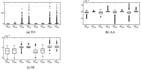
Figure 1. Box-whisker plots of the observed distributions of (a) TO, (b) AA, and (c) SE values for the optimized portfolios P${}_{\alpha }^0$ through P${}_{\alpha }^3$.

Figure 2 shows the price performance of the base portfolios, P${}_{0.95}^0$ and P${}_{0.99}^0$, under change of turnover constraint. We note the relative insensitivity of price performance of P${}_{0.95}^0$ to the changing TO constraint. The price performance is more sensitive at the $\alpha =0.99$ quantile level.

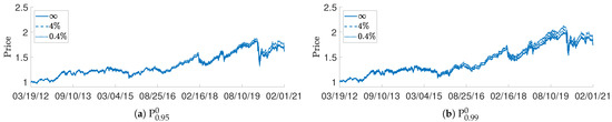
Figure 2. Cumulative price performance of the P${}_{0.95}^0$ and P${}_{0.99}^0$ portfolios under changing TO constraint level.

Figure 3 shows the cumulative price performance of each of the performance attribute constrained, CVaR${}_{0.95}$ minimized portfolios under changing TO constraint level computed using both the EQW (left plots) and PW (right plots) benchmarks to determine AA and SE values. As with the base portfolio, the price performance of the AA-constrained portfolio P${}_{0.95}^1$ is relatively insensitive to changing the TO constraint level. Much greater sensitivity is seen in the price performance of the SE-constrained portfolio P${}_{0.95}^2$ for the EQW benchmark. In contrast, the price performance is relatively insensitive to $C_{\mathrm{TO}}$ for P${}_{0.95}^2$ computed with the PW benchmark. Since the SE constraint affects the sensitivity of the total excess return to the weighting of assets within each individual asset class we ascribe this sensitivity difference as due to the difference in asset weighting between the EQW and a PW benchmark portfolios. The sensitivity of P${}_{\alpha }^3$ to changing the TO constraint level reflects a “compromise” between the sensitivity of the AA-constrained P${}_{\alpha }^1$ and the SE constrained P${}_{\alpha }^2$. For both $\alpha =0.95$ and $\alpha =0.99$, the result is that the price performance of the doubly constrained portfolio improves under tighter daily TO constraint.

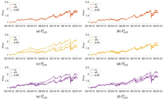
Figure 3. Cumulative price performance of each of the CVaR_0.95 minimized portfolios under changing TO constraint level; (left) equi-weighted benchmark, (right) price-weighted benchmark.

Figure 4 summarizes the cumulative price performance of the CVaR${}_{0.95}$ minimized portfolios under the TO $\le 0.4\%$ constraint level for both the EQW and PW benchmarks. For both benchmark valuations, we see that the AA-constrained portfolio, P${}_{0.95}^1$, produces only slight price performance improvement compared to the base portfolio. For both benchmarks, the AA and SE constrained portfolio, P${}_{0.95}^3$, produces strong improved price performance compared to the base portfolio. For the reason attributed above, the price performance improvement for the SE-constrained portfolio, P${}_{0.95}^2$, is different between the EQW and PW portfolios.

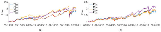
Figure 4. Cumulative price performance of the CVaR_0.95 minimized portfolios under the TO ≤ 0.4% constraint level; (a) equi-weighted benchmark, (b) price-weighted benchmark.

Figure 5 summarizes total time period risk measures for the $\alpha =0.95$ portfolios constrained by a daily turnover of 0.4%. The reported maximum drawdowns all reflect behavior related to the onset of the Covid-19 pandemic. Our optimized portfolios all outperform the benchmarks in MDD, but only the P${}_{0.95}^2$ portfolio using PW benchmark valuations for SE outperforms the base portfolio P${}_{0.95}^0$. Surprisingly, the benchmarks have better Sharpe ratios than any of the optimized portfolios. However, all of the performance attribute constrained portfolios outperform the base portfolio. For the EQW benchmark, all optimized portfolios have better Sortino–Satchell ratios than the benchmarks. For both EQW and PW, the SE-constrained portfolios also outperform those of the base portfolio. All optimized portfolios equal or are better than the Rachev ratios of the benchmarks. The SE-constrained portfolio using PW benchmark valuation also outperforms that of the base portfolio.

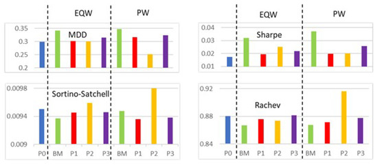
Figure 5. Total time period risk measures for the $\alpha =0.95$ portfolios constrained by a daily turnover of 0.4%. (BM = benchmark; P0 = P${}_{0.95}^0$, etc.).

4. Discussion

It is well-known that no single optimization method can achieve all goals. Compared with the CVaR optimizations P${}_{\alpha }^0$ which impose no performance attribution constraints, the price and risk measure performances of the three performance-constrained CVaR${}_{\alpha }$ optimizations, each computed at two values of $\alpha =095,0.99$, considered in this study lead to the following observations.

• The constraint $\mathrm{AA}\ge 0$ is easiest to impose in the following sense. The base case had ∼60% negative daily AA values, while AA-constrained portfolios achieved essentially 100% non-negative AA values with minimal frequency of “softening” of either the AA or TO constraint.
• The constraint $\mathrm{SE}\ge 0$ is harder to impose; there was significant coupling between the turnover and SE constraints. The base case had ∼90% negative daily SE values. Achieving $<5\%$ negative daily SE values required significantly frequent softening of the daily turnover constraint.
• Price performance improvement compared to the base portfolio was best achieved by imposing both AA and SE constraints.
• The SE-constrained portfolio P${}_{\alpha }^2$ tended to perform best with respect to the four risk measures considered.

References

- Artzner, Phillipe, Freddy Delbaen, Jean-Marc Eber, and David Heath. 1999. Coherent measures of risk. Risk 10: 203–28. [Google Scholar] [CrossRef]
- Bacon, Carl R. 2008. Practical Portfolio Performance: Measurement and Attribution, 2nd ed. West Sussex: John Wiley and Sons. [Google Scholar]
- Biglova, Almira, and Svetlozar T. Rachev. 2007. Portfolio performance attribution. Investment Management and Financial Innovations 4: 7–22. [Google Scholar]
- Brinson, Gary P., and Nimrod Fachler. 1985. Measuring non-United-States equity portfolio performance. The Journal of Portfolio Management 11: 73–76. [Google Scholar] [CrossRef]
- Brinson, Gary P., L. Randolph Hood, and Gilbert L. Beebower. 1986. Determinants of portfolio performance. Financial Analysts Journal 42: 39–44. [Google Scholar] [CrossRef]
- Cherdito, Patrick, and Eduard Kromer. 2013. Reward-risk ratios. Journal of Investment Strategies 3: 1–16. [Google Scholar] [CrossRef]
- Gava, Jerome, Francisco Guevara, and Julien Turc. 2021. Turning tail risks into tailwinds. The Journal of Portfolio Management ‘Multi-Asset’ Special Edition 47: 41–70. [Google Scholar] [CrossRef]
- JP Morgan. 1996. Risk Metrics Technical Manual, 4th ed. New York: JP Morgan. [Google Scholar]
- Konno, Hiroshi, and Hiroaki Yamazaki. 1991. Mean-absolute deviation portfolio optimization model and its application to Tokyo stock market. Management Science 37: 519–31. [Google Scholar] [CrossRef]
- Markowitz, Harry. 1952. Portfolio selection*. Journal of Finance 7: 77–91. [Google Scholar]
- Pflug, George C. 2000. Some remarks on the value-at-risk and the conditional value-at-risk. In Probabilistic Constrained Optimization. Edited by Stanislav P. Uryasev. Nonconvex Optimization and Its Applications. Boston: Springer, Vol. 49, pp. 272–81. [Google Scholar]
- Rachev, Svetlozar T., R. Douglas Martin, Borjana Racheva, and Stoyan Stoyanov. 2009. Stable ETL optimal portfolios and extreme risk management. In Risk Assessment. Heidelberg: Physica-Verlag HD, pp. 235–62. [Google Scholar]
- Rachev, Svetlozar T., Stoyan Stoyanov, and Frank J. Fabozzi. 2008. Advanced Stochastic Models, Risk Assessment, and Portfolio Optimization. Hoboken: John Wiley and Sons. [Google Scholar]
- Rockafellar, R. Tyrrell, and Stanislav Uryasev. 2000. Optimization of conditional value-at-risk. Journal of Risk 2: 21–41. [Google Scholar] [CrossRef]
- Sharpe, William F. 1994. The Sharpe ratio. Journal of Portfolio Management 21: 49–58. [Google Scholar] [CrossRef]
- Sortino, Frank A., and Stephen Satchell. 2001. Managing Downside Risk in Financial Markets. Oxford: Butterworth-Heinemann. [Google Scholar]
- Stoyanov, Stoyan V. 2005. Optimal Portfolio Management in Highly Volatile Markets. Ph.D. thesis, Karlsruhe Institute of Technology, Karlsruhe, Germany. [Google Scholar]