
Portfolio Optimization Constrained by Performance Attribution


Abstract
1. Introduction
2. Description of the Approach
- If , the expected return from asset class i in the benchmark is outperforming the total expected return for the benchmark. Therefore if , the weight of asset class i in portfolio p is larger than in the benchmark, capitalizing further on the better return from class i. Otherwise, if , the class i weighting in portfolio p is hurting the potential performance of that class (as determined by the benchmark).
- If , the expected return from asset class i in the benchmark is under-performing the total expected return for the benchmark. Therefore if , the weight of asset class i in portfolio p is smaller than in the benchmark, further suppressing the poorer return from that class. Otherwise, if , the class i weighting in portfolio p is overweighting the poor performance of that class.
- P:
- (a) ; and (b)
- P:
- (a) ; (b) ; and (c) .
- P:
- (a) ; (b) ; and (d) .
- P:
- (a) ; (b) ; (c) ; and (d) .
- maximum drawdown (MDD),which characterizes the maximum loss incurred from peak to trough during the time period ;
- Sharpe ratio (Sharpe 1994),where is a risk-free rate, and and are the expected mean and standard deviation of the portfolio’s excess return, ;
- Sortino–Satchell ratio (Sortino and Satchell 2001),and
- Rachev ratio (Rachev et al. 2008),which represents the reward potential for positive returns compared to the risk potential for negative returns at quantile levels defined by the user. In our analysis, we set .
3. Application to a Test Portfolio
- P:
- The turnover constraint was replaced by a penalty term.
- P:
- The turnover constraint was replaced by a penalty term. If the feasible set was still null, the asset allocation constraint was then additionally replaced by a penalty term.
- P:
- The turnover constraint was replaced by a penalty term; if necessary, the selection effect constraint was also replaced.
- P:
- The order of additional conversion to penalty terms was turnover constraint, selection effect, and finally asset allocation.
4. Discussion
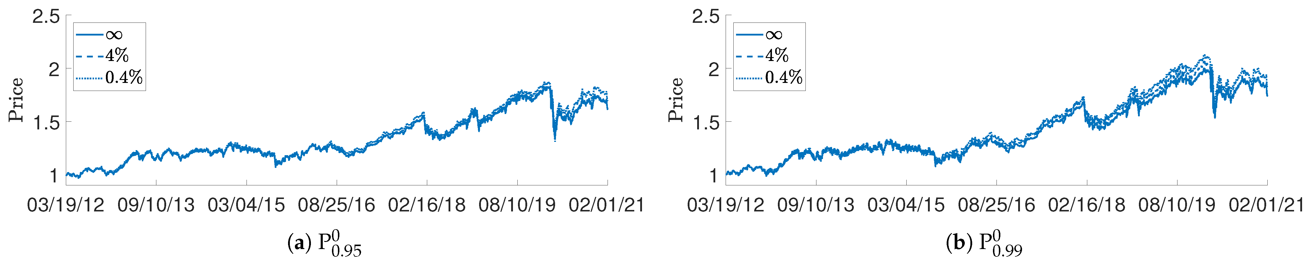
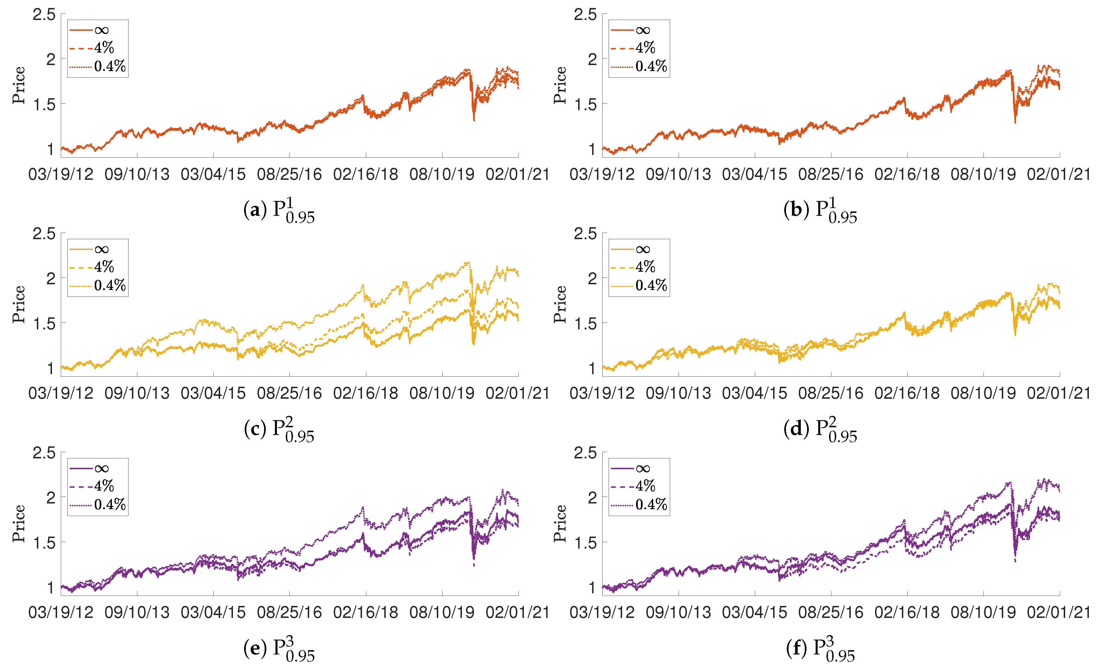
- The constraint is easiest to impose in the following sense. The base case had ∼60% negative daily AA values, while AA-constrained portfolios achieved essentially 100% non-negative AA values with minimal frequency of “softening” of either the AA or TO constraint.
- The constraint is harder to impose; there was significant coupling between the turnover and SE constraints. The base case had ∼90% negative daily SE values. Achieving negative daily SE values required significantly frequent softening of the daily turnover constraint.
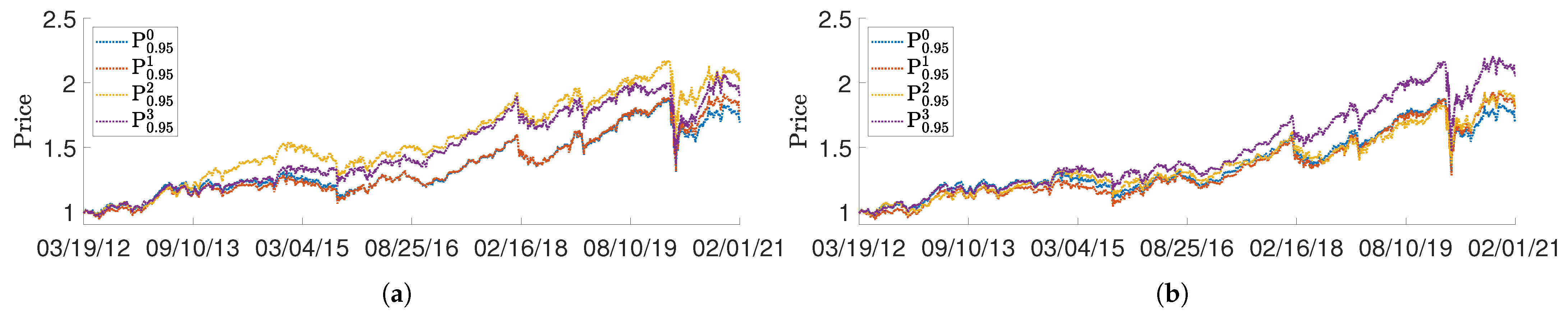
- Price performance improvement compared to the base portfolio was best achieved by imposing both AA and SE constraints.
- The SE-constrained portfolio P tended to perform best with respect to the four risk measures considered.
Author Contributions
Funding
Data Availability Statement
Conflicts of Interest
Appendix A

| Ticker | Company | Inception | Weight | Ticker | Company | Inception | Weight |
|---|---|---|---|---|---|---|---|
| Date | (%) | Date | (%) | ||||
| UNH | UnitedHealth | 10/16/1984 | 7.27 | TRV | Travelers Cos. | 11/16/1975 | 3.01 |
| GS | Goldman Sachs | 05/03/1999 | 5.98 | NKE | NIKE | 12/01/1980 | 2.96 |
| HD | Home Depot | 09/21/1981 | 5.88 | APPL | Apple | 12/11/1980 | 2.92 |
| AMGN | Amgen | 07/16/1983 | 5.23 | JPM | JPMorgan Chase | 03/16/1990 | 2.82 |
| MSFT | Microsoft | 03/12/1986 | 5.21 | PG | Procter and Gamble | 01/01/1962 | 2.81 |
| CRM | salesforce.com | 07/22/2004 | 4.97 | IBM | Int’l Business Mach. | 01/01/1962 | 2.63 |
| MCD | McDonald’s | 07/04/1966 | 4.52 | AXP | American Express | 03/31/1972 | 2.55 |
| V | Visa | 03/18/2008 | 4.31 | CVX | Chevron | 01/01/1962 | 1.88 |
| BA | Boeing | 01/01/1962 | 4.26 | MRK | Merck and Co. | 01/01/1970 | 1.68 |
| HON | Honeywell Int’l. | 01/01/1970 | 4.25 | INTC | Intel | 03/16/1980 | 1.23 |
| CAT | Caterpillar | 01/01/1962 | 4.02 | VZ | Verizon Commun. | 11/20/1983 | 1.18 |
| MMM | 3M | 01/01/1970 | 3.8 | DOW | Dow | 03/20/2019 | 1.15 |
| DIS | Walt Disney | 01/01/1962 | 3.72 | WBA | Walgreens Boots All. | 03/16/1980 | 1.06 |
| JNJ | Johnson and Johnson | 01/01/1962 | 3.54 | KO | Coca-Cola | 01/01/1962 | 1.06 |
| WMT | Walmart | 08/24/1972 | 3.03 | CSCO | Cisco Systems | 02/15/1990 | 0.99 |
References
- Artzner, Phillipe, Freddy Delbaen, Jean-Marc Eber, and David Heath. 1999. Coherent measures of risk. Risk 10: 203–28. [Google Scholar] [CrossRef]
- Bacon, Carl R. 2008. Practical Portfolio Performance: Measurement and Attribution, 2nd ed. West Sussex: John Wiley and Sons. [Google Scholar]
- Biglova, Almira, and Svetlozar T. Rachev. 2007. Portfolio performance attribution. Investment Management and Financial Innovations 4: 7–22. [Google Scholar]
- Brinson, Gary P., and Nimrod Fachler. 1985. Measuring non-United-States equity portfolio performance. The Journal of Portfolio Management 11: 73–76. [Google Scholar] [CrossRef]
- Brinson, Gary P., L. Randolph Hood, and Gilbert L. Beebower. 1986. Determinants of portfolio performance. Financial Analysts Journal 42: 39–44. [Google Scholar] [CrossRef]
- Cherdito, Patrick, and Eduard Kromer. 2013. Reward-risk ratios. Journal of Investment Strategies 3: 1–16. [Google Scholar] [CrossRef]
- Gava, Jerome, Francisco Guevara, and Julien Turc. 2021. Turning tail risks into tailwinds. The Journal of Portfolio Management ‘Multi-Asset’ Special Edition 47: 41–70. [Google Scholar] [CrossRef]
- JP Morgan. 1996. Risk Metrics Technical Manual, 4th ed. New York: JP Morgan. [Google Scholar]
- Konno, Hiroshi, and Hiroaki Yamazaki. 1991. Mean-absolute deviation portfolio optimization model and its application to Tokyo stock market. Management Science 37: 519–31. [Google Scholar] [CrossRef]
- Markowitz, Harry. 1952. Portfolio selection*. Journal of Finance 7: 77–91. [Google Scholar]
- Pflug, George C. 2000. Some remarks on the value-at-risk and the conditional value-at-risk. In Probabilistic Constrained Optimization. Edited by Stanislav P. Uryasev. Nonconvex Optimization and Its Applications. Boston: Springer, Vol. 49, pp. 272–81. [Google Scholar]
- Rachev, Svetlozar T., R. Douglas Martin, Borjana Racheva, and Stoyan Stoyanov. 2009. Stable ETL optimal portfolios and extreme risk management. In Risk Assessment. Heidelberg: Physica-Verlag HD, pp. 235–62. [Google Scholar]
- Rachev, Svetlozar T., Stoyan Stoyanov, and Frank J. Fabozzi. 2008. Advanced Stochastic Models, Risk Assessment, and Portfolio Optimization. Hoboken: John Wiley and Sons. [Google Scholar]
- Rockafellar, R. Tyrrell, and Stanislav Uryasev. 2000. Optimization of conditional value-at-risk. Journal of Risk 2: 21–41. [Google Scholar] [CrossRef]
- Sharpe, William F. 1994. The Sharpe ratio. Journal of Portfolio Management 21: 49–58. [Google Scholar] [CrossRef]
- Sortino, Frank A., and Stephen Satchell. 2001. Managing Downside Risk in Financial Markets. Oxford: Butterworth-Heinemann. [Google Scholar]
- Stoyanov, Stoyan V. 2005. Optimal Portfolio Management in Highly Volatile Markets. Ph.D. thesis, Karlsruhe Institute of Technology, Karlsruhe, Germany. [Google Scholar]
| 1. | In the original formulation by Brinson et al. (1986) (see also Chapter 5 in Bacon (2008)), is defined as . The definition in Biglova and Rachev (2007), which we follow here, uses the excess return for benchmark class i relative to the entire benchmark return in the definition (1) of . While this modifies the values for relative to that of the original Brinson et al. formulation, we note that the total value, , is in agreement with the total value of in the Brinson et al. approach. |
| 2. | If and were simple (i.e., discrete) returns, formulas of the form (3) are exact. However, as they are log-returns, such formulas are approximate. For example, the formula for incurs an error term which, to leading order in a Taylor series expansion, is . |
| 3. | A requirement for class i to be in the portfolio. |
| 4. | If the underlying profit-loss distribution is continuous, then the definitions of ETL (also known as tail conditional expectation (TCE) or tail value-at-risk (TVaR)) and CVaR (also known as expected shortfall (ES) or average value-at-risk (AVaR)) coincide. In the general case however, CVaR is a coherent risk measure while ETL is not (Stoyanov 2005). |
| 5. | We adopt the convention that loss is negative valued and that and have negative values in the case of loss. |
| 6. | see Note 5. |
| 7. | see Note 5. |
| 8. | This assumes that benchmark weight values can be obtained in a timely manner and are not part of the optimization. |
| 9. | Specifically is the optimized weight to be applied to the portfolio at the beginning of (and throughout the entire) day t. |
| 10. | see Note 2. |
| 11. | We exclude Dow Inc. which was spun off of DowDuPont on 1 April 2019. Its stock, under the ticker symbol “DOW”, began trading on 20 March 2019. It was added to the DJIA on 2 April 2019. |
| 12. | Bloomberg Professional Services. |
| 13. | Thus Q = N and = , . |
| 14. | Table 2 shows the results for the PW benchmark; as noted, the results for the EQW benchmark are essentially the same. |


| Class | Stock Ticker | Class Weight in DJIA(%) |
|---|---|---|
| 1 | UNH, GS, HD, AMGN, MSFT | |
| 2 | CRM, MCD, V, BA, HON | |
| 3 | CAT, MMM, DIS, JNJ, WMT | |
| 4 | TRV, NKE, AAPL, JPM, PG | |
| 5 | IBM, AXP, CVX, MRK, INTC | |
| 6 | VZ, WBA, KO, CSCO |
| Portfolio | All ‘Hard’ | TO | TO+AA | TO+SE | TO+SE+AA | no Solution for t |
|---|---|---|---|---|---|---|
| TO | ||||||
| P | 100.00% | 0.00% | ||||
| P | 100.00% | 0.00% | 0.00% | |||
| P | 44.11% | 55.84% | 0.04% | |||
| P | 54.90% | 42.99% | 1.93% | 0.18% | ||
| TO ≤ 4% | ||||||
| P | 99.87% | 0.13% | 0.00% | |||
| P | 98.61% | 1.39% | 0.00% | 0.00% | ||
| P | 41.24% | 12.58% | 46.13% | 0.04% | ||
| P | 45.54% | 19.03% | 34.39% | 1.03% | 0.00% | |
| TO ≤ 0.4% | ||||||
| P | 78.15% | 21.85% | 0.00% | |||
| P | 51.68% | 48.32% | 0.00% | 0.00% | ||
| P | 6.85% | 87.51% | 5.64% | 0.00% | ||
| P | 6.76% | 90.06% | 3.00% | 0.18% | 0.00% | |
Publisher’s Note: MDPI stays neutral with regard to jurisdictional claims in published maps and institutional affiliations. |
© 2021 by the authors. Licensee MDPI, Basel, Switzerland. This article is an open access article distributed under the terms and conditions of the Creative Commons Attribution (CC BY) license (https://creativecommons.org/licenses/by/4.0/).
Share and Cite
Hu, Y.; Lindquist, W.B.; Rachev, S.T. Portfolio Optimization Constrained by Performance Attribution. J. Risk Financial Manag. 2021, 14, 201. https://doi.org/10.3390/jrfm14050201
Hu Y, Lindquist WB, Rachev ST. Portfolio Optimization Constrained by Performance Attribution. Journal of Risk and Financial Management. 2021; 14(5):201. https://doi.org/10.3390/jrfm14050201
Chicago/Turabian StyleHu, Yuan, W. Brent Lindquist, and Svetlozar T. Rachev. 2021. "Portfolio Optimization Constrained by Performance Attribution" Journal of Risk and Financial Management 14, no. 5: 201. https://doi.org/10.3390/jrfm14050201
APA StyleHu, Y., Lindquist, W. B., & Rachev, S. T. (2021). Portfolio Optimization Constrained by Performance Attribution. Journal of Risk and Financial Management, 14(5), 201. https://doi.org/10.3390/jrfm14050201