Abstract
Recently, a large number of empirical studies indicated that individual equity options exhibit a strong factor structure. In this paper, the importance of systematic and idiosyncratic volatility and jump risks on individual equity option pricing is analyzed. First, we propose a new factor structure model for pricing the individual equity options with stochastic volatility and jumps, which takes into account four types of risks, i.e., the systematic diffusion, the idiosyncratic diffusion, the systematic jump, and the idiosyncratic jump. Second, we derive the closed-form solutions for the prices of both the market index and individual equity options by utilizing the Fourier inversion. Finally, empirical studies are carried out to show the superiority of our model based on the S&P 500 index and the stock of Apple Inc. on options. The out-of-sample pricing performance of our proposed model outperforms the other three benchmark models especially for short term and deep out-of-the-money options.
JEL Classification:
G13
1. Introduction
Most of the existing literature studies on option pricing are for index options, and there are very few about equity options. One approach to modeling equity options is to employ the state-of-the-art model in the index option literature, a stochastic volatility model with jumps (see, for example, , ; ; ; ; ; ; ; ), but to ignore any underlying factor structure.
In (), the research results indicated that the volatility risk premium is negative in index options by examining the statistical properties of delta hedged option portfolios, i.e., a portfolio of a long call option position hedged by a short position in the stock. On the one hand, stock returns have a significant market component; the emergence of market volatility risk premiums is bound to have an impact on individual equity option pricing. On the other hand, from the economic point of view, the risk neutral distributions of individual equities are systematically different from the market index. Thus, it is necessary to explore how volatility risk is priced in individual equity options, which also can produce additional insights into the pricing structure of individual equity options (see ). As is well known, the beta of a stock represents the sensitivity of the risk of the individual equity with respect to the systematic risk of the market and is very useful for portfolio construction in the capital asset pricing model. Therefore, under the assumption that stock returns include a market component and an idiosyncratic component, () developed a factor model for equity option valuation and investigated the pricing of market volatility risk in individual equity options. Their empirical results showed that volatility risk premiums in equity options are smaller than in index options.
Afterwards, () proposed a continuous-time capital asset pricing model (CAPM) where the dynamics of the market index have a stochastic volatility driven by a fast mean reverting process. Moreover, they derived the analytical approximation pricing formulas for both the market index and individual equity call options using a singular perturbation method. Meanwhile, a calibration method for the beta parameter was also presented based on the estimated model parameters of both the market index and individual equity option prices. Subsequently, () extended the constant beta-parameter factor model of () by considering a piecewise-linear relationship between the individual asset and the market index and proposed a regime switching factor model for the pricing market index and individual equity options. Supposing that stock return is linearly related to market index return in terms of the beta parameter, () developed a factor model for individual equity option pricing under a purely discontinuous Lévy process via fast Fourier transform, in which the variance gamma process for the dynamics of both the market index and stock was taken as an example for illustration. By supposing a continuous-time CAPM with Lévy processes, () also derived analytical solutions to the index and equity options and explored the corresponding static hedging with index futures. () empirically studied the equity volatility levels, skews, and term structures by using equity option prices and principal component analysis. The results indicated that the equity options had a strong factor structure, and then, they developed an equity option pricing model with a CAPM factor structure and stochastic volatility, which allowed for mean reverting stochastic volatility for the dynamics of both the market factor and individual equity.
Recently, () proposed a GARCH-jump model for individual stock returns that took into account four types of risks: the systematic and idiosyncratic jumps and the systematic and idiosyncratic diffusive volatility. By using a dataset consisting of the S&P 500 index and 15 individual stock prices, their empirical results indicated that idiosyncratic jumps were a key determinant of expected stock return.1 Instead of using only stock returns, () used both stock and option data to decompose the four risk premiums associated with systematic and idiosyncratic diffusive and jump risks and also documented that idiosyncratic jumps are important determinants of the mean returns of a stock from both an ex post and ex ante perspective.
Motivated by the above mentioned insights, we propose to price individual equity options in stochastic volatility jump-diffusion models with a market factor structure, which can be seen as a generalized version of (). Specifically, in our proposed model, the individual equity prices are driven by the market factor, as well as an idiosyncratic component that also has stochastic volatility and jump. Due to the model belonging to the affine class, we derive the closed-form solutions for the prices of both the market index and individual equity options by utilizing the Fourier inversion. In addition, we provide the empirical results to test the pricing performance of the proposed factor model based on the S&P 500 index and the stock of Apple Inc. (AAPL) on options. Toward this end, we empirically compare the pricing performance of the proposed model with those of the other three classical two factor stochastic volatility models being taken as benchmark models. Empirical results presented here confirm that the equity option pricing model considering systematic and idiosyncratic volatility and jump risks may offer a good competitor to the models of (), (), or () for some other option markets.
The remainder of the paper proceeds as follows. In Section 2, we present a novel factor model for equity option valuation and derive the corresponding closed-form solutions. In Section 3, empirical studies are carried out to show the pricing performance of our proposed model. Finally, some conclusions are stated in Section 4.
2. Equity Option Valuation
In this section, we introduce a general class of stochastic volatility models with jumps for the dynamics of both the market factor and individual equity prices and derive closed form solutions to the prices of the European equity call and put options.
2.1. Model Description
Consider a filtered probability space with information filtration satisfying the usual conditions (increase, right-continuous, and augmented), where is a risk neutral measure. We model an equity market consisting of N firms with a single market factor, (usually approximated by a market index in practice). The individual stock prices are denoted by , for . For the sake of convenience, we ignore the superscript i, and denote the pricing process of an individual stock. Investors also have access to a risk free bond that pays a return rate of r. To start, the market factor evolves under a risk neutral measure as:
where stands for the value of before a possible jump occurs, , is the variance of market factor, denotes the long run variance, captures the mean reversion speed of to , measures the volatility of volatility, to ensure that the process remains strictly positive2, and are correlated standard Brownian motions, i.e., the innovations to the market return and volatility are correlated with correlation coefficient , , and is a compensated jump measure, where is the jump measure and the Lévy kernel (or density) satisfies .
Furthermore, we separate the effects of the market factor on individual equities’ returns into two types of risks: the systematic diffusive volatility and jump. More specifically, the diffusive random variation of individual equities’ returns is dependent on the Brownian motion that drives market returns through the coefficient . In addition, the discontinuous movements in the market return can also trigger jumps in individual equities’ returns through the coefficient . Therefore, the individual equity prices are driven by the market factor, as well as an idiosyncratic component that also has stochastic volatility and jump, whose process under a risk neutral measure follows:3
where stands for the value of before a possible jump occurs, , is the idiosyncratic variance of individual equity, denotes the long run idiosyncratic variance, captures the mean reversion speed of to , measures the volatility of idiosyncratic variance, to ensure that the process remains strictly positive4, and are correlated standard Brownian motions, i.e., the innovations to the idiosyncratic return and volatility are correlated with correlation coefficient , , but they are independent of Brownian motions in the market factor, i.e., for , and is a compensated jump measure, where is the jump measure and the Lévy kernel (or density) satisfies .
2.2. Characteristic Function
In order to be able to derive the pricing formulas for the European call and put equity options, we are particularly interested in the characteristic function of the logarithm asset price. Given the dynamics of the underlying asset price under the measure, we consider the conditional characteristic function of log-asset price given the market information up to time t, which is denoted by :
where denotes the condition expectation under the measure, , and .
Lemma 1.
Suppose that the market factor and individual equity price are driven by Equations (1) and (3), respectively. Then, the conditional characteristic function of log-asset price is given by:
where:
and .
Proof.
To obtain the conditional characteristic function of log-asset price , we first take the following transformation by using the Itô lemma for Equation (3):
The Feynman–Kac formula states that is governed by the following partial integro-differential equation (PIDE):
Due to the affine structure of our model, we postulate admitting the form of (6). Substituting Equation (6) into the above PIDE (7) gives the following system of ordinary differential equations (ODEs) for , , , and :
where the boundary conditions are given as and .
By solving the above ODEs, we can obtain the characteristic function (6). □
Lemma 2.
Suppose that the market factor is driven by Equation (1). Then, the conditional characteristic function of log-market factor is given by:
where:
and .
Proof.
Similar to the proof of Lemma 1, we can easily verify the above results. □
2.3. Valuation of the European Index and Equity Options
Once the characteristic function is found, it is straightforward to calculate the prices of European options by using Fourier inversion. Let and be the prices of the European equity call and put options at time t with strike price K and maturity T under the risk neutral measure , respectively. Then, these option prices are determined by:
and:
where is the time to maturity.
Theorem 1.
Suppose that the market factor and the individual equity price are driven by Equations (1) and (3), respectively. Then, the prices of the European equity call and put options with strike price K and maturity are given by:
and:
where the risk neutral probability distribution functions and are defined by:
and:
where is the conditional characteristic function of , which can be seen in Equation (6), and indicates the real part of a complex number.
Proof.
In order to get the pricing formulas of the European equity call and put options, let us first introduce a change of measure from to by the following Radon–Nikodym derivative:
We denote the conditional characteristic function of under the measure by . Then, can be expressed as:
Thus, the price of a European equity call option can be calculated by utilizing and :
Once the conditional characteristic function is obtained, we can easily calculate the probability distribution functions and according to the Lévy inversion formula:
and:
A similar approach can be used to derive the pricing formula for the European equity put option. □
In a similar way, we also can present the pricing formulas for the European index call and put options.
Theorem 2.
Suppose that the market factor is driven by Equation (1). Then, the time t prices of the European index call and put options with strike price K and maturity are given by:
and:
where the risk neutral probability distribution functions and are defined by:
and:
where is the conditional characteristic function of , which can be seen in Equation (8).
3. Empirical Studies
In this section, we empirically compare the pricing performance of our proposed model with those of the classical two factor stochastic volatility models, such as () (two variance SVmodel with price jumps, 2-SVJmodel), () (two-variance SV model, 2-SV model), and () (two-variance SV model with a single market factor, 2-FSVmodel), being taken as benchmark models.
3.1. Data Description
We used the S&P 500 index (SPX) to proxy for the market factor and AAPL as the individual equity. We employed the delayed market quotes on arbitrary date 8 May 2019, which was the last date available at the time of writing, as the in-sample data to calibrate the risk neutral parameters, and those on 9 May 2019 were used for the out-of-sample test. We used mid-quotes to represent the option prices. To eliminate the sample noise in raw option data, we adopted some filtering rules commonly used within the related literature: (i) we omitted those options with fewer than seven days and more than 365 days to maturity; (ii) all observations with zero trading volume were discarded; (iii) all options with implied volatility equal to zero and larger than 1.0 were discarded. In addition, for the convenience of the empirical analysis in the following, we only considered the sample data of the index call options and individual equity call options with the same expiration date. Thus, we focused only on ten maturities slices, namely on the maturities of 24 May 2019, 31 May 2019, 7 June 2019, 14 June 2019, 21 June 2019, 19 July 2019, 16 August 2019, 20 September 2019, 18 October 2019, and 17 January 2020.
After these filters, we had a total of 401 observations for the S&P 500 index call option on 8 May 2019. The individual equity option sample contained 233 call options on 8 May 2019 and 264 call options on 9 May 2019, respectively. Due to the life of an option being usually less than one year, we chose the three month U.S. Treasury Bill Rate to substitute for the risk free interest rate. All of the data were downloaded from the Chicago Board Options Exchange (http://www.cboe.com/).
3.2. Parameter Estimation
Our proposed model allowed a general distribution for jump components of the market factor and individual equity price and thus could be easily introduced to the special cases such that the jump components follow the compound Poisson process of () and (), etc. For different types of Lévy kernels, different forms of our model can be presented. In order to keep consistent with () for comparative analysis, in the following, we assumed that the jump components of the dynamics for the market factor and individual equity followed compound Poisson processes and the jump magnitude was drawn from the log-normal distribution of (). Thus, the Lévy kernels for the market factor and individual equity, respectively, are given by:
and:
where , for , denotes the jump intensity, is the mean of the jump size, and is the variance of the jump size. Then, the integrals , for , in Lemmas 1 and 2 can be calculated as follows:
and
Based on Theorems 1 and 2, we employed a two step calibration procedure (see, for example, ; ) to estimate the model parameters. First, we calibrated the market index dynamic based on the S&P 500 index option price alone. Second, we used the equity option price to calibrate the individual equity dynamic conditional on estimates of . Consider the situation in which an investor wants to hedge his or her equity position with index options and hedging horizon T. For brevity, we further suppose that the investor observes index option prices and equity option prices both with maturity T, the same as hedging horizon. Specifically, the dataset contains index option prices , for , and equity option prices , for .
In the calibration process, the risk neutral model parameters were backed out by minimizing a loss function capturing the fit between the theoretical model and market prices. We employed the root mean squared errors (RMSE) as the objective function. The first step calibrated the risk neutral parameters for the index process, which are calibrated by:
where is the market price of the index call option contract from the sample and represents the model price calculated using Equation (15) and the vector of model input parameters .
The second calibrated the beta and the parameters for the idiosyncratic risk:
where is the market price of the equity call option contract from the sample and represents the model price calculated using Equation (13) and the vector of model input parameters .
On the basis of the above calibration method, Table 1 presents the risk neutral parameter estimates across various model specifications. Note that the values of the diffusive beta and jump beta for our proposed model were 0.3891 and 0.8429, respectively. The corresponding value of for the 2-FSV model was 0.2457. Obviously, both our proposed model and the 2-FSV model showed that AAPL tended to have a relatively low exposure to diffusive market movements. However, the jump exposure coefficient indicated that the AAPL had a strong exposure to market jumps, which meant that the factor structure of the jumps was much stronger than the one of the diffusive movements. The reason for this result may be related to the sample data we selected. If we can get more sample data in the future, we will do an in-depth analysis. Moreover, we also can see that the values of correlation were strongly negative for four models, capturing the so-called leverage effect both in the index and individual equity.
Table 1.
Estimated parameters. Note: This table shows the average of the estimated parameters obtained by minimizing the root mean squared pricing errors between the market price and the model price for each option on 8 May 2019. Standard errors are reported in parentheses.
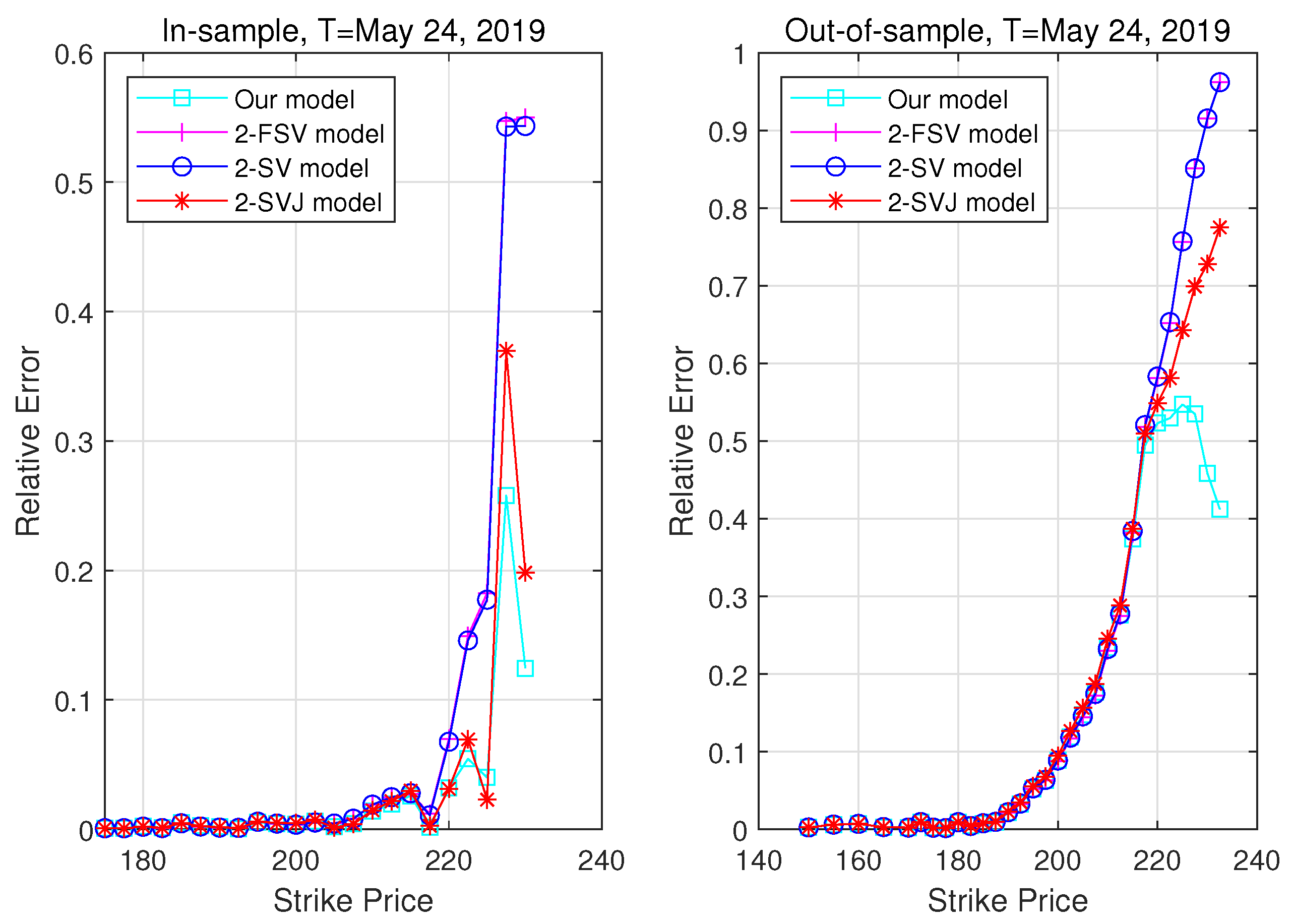
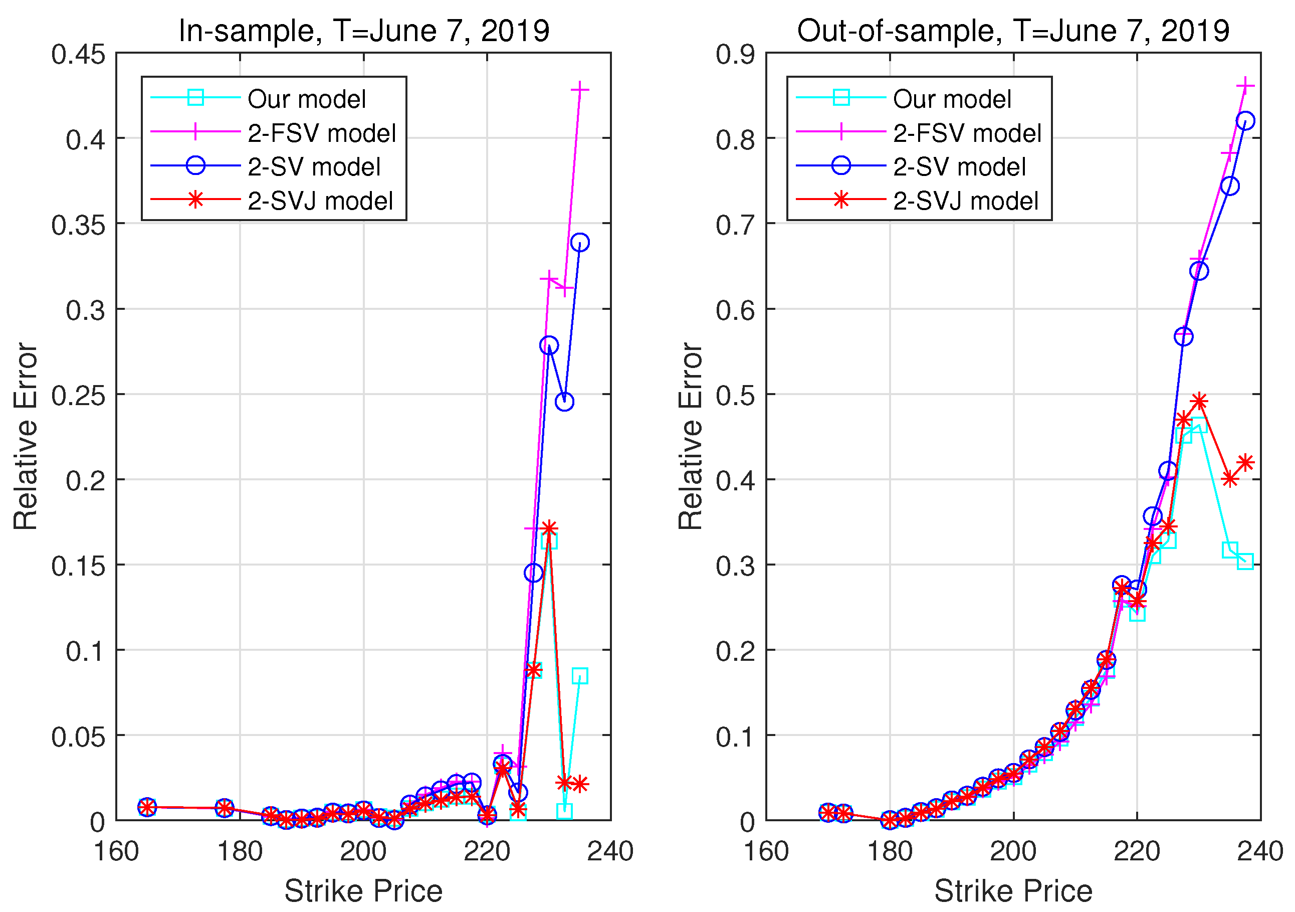
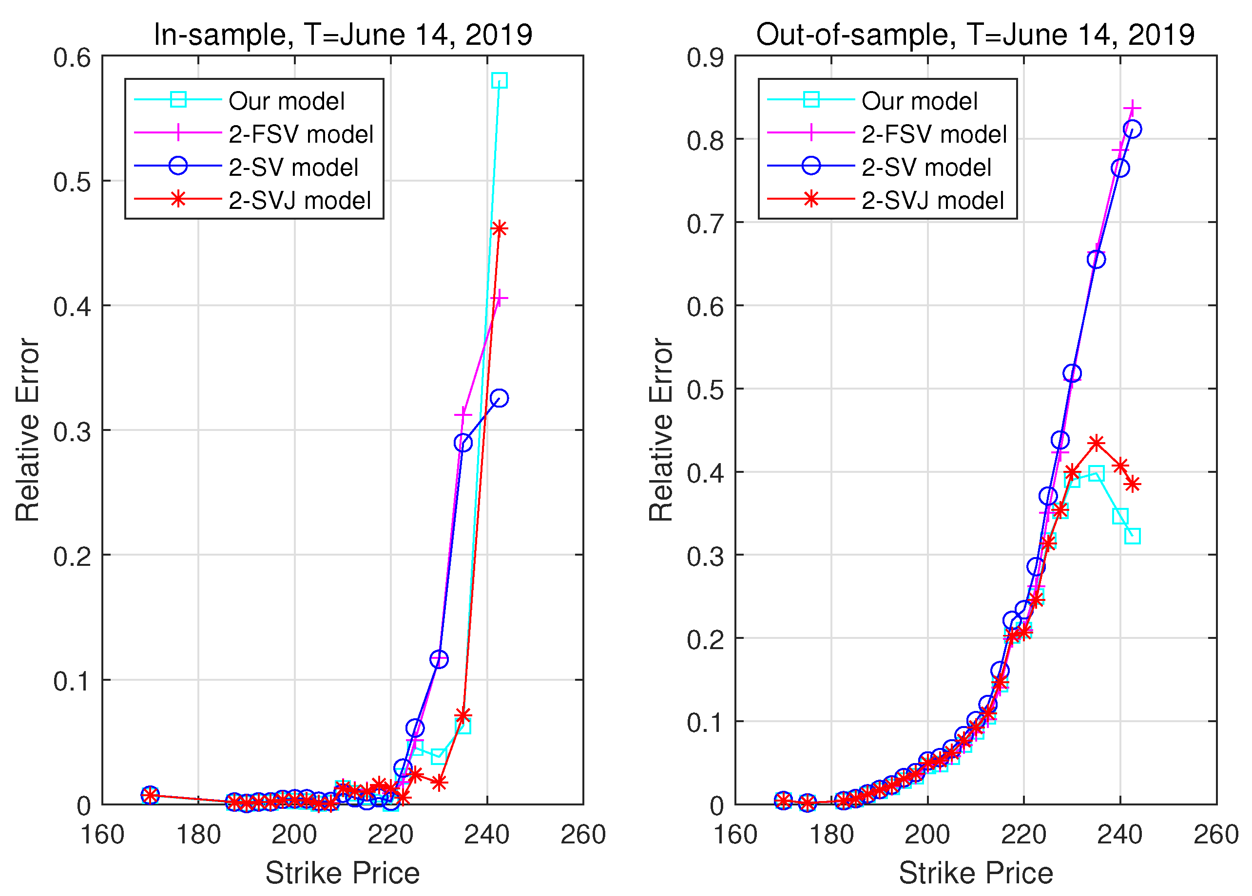
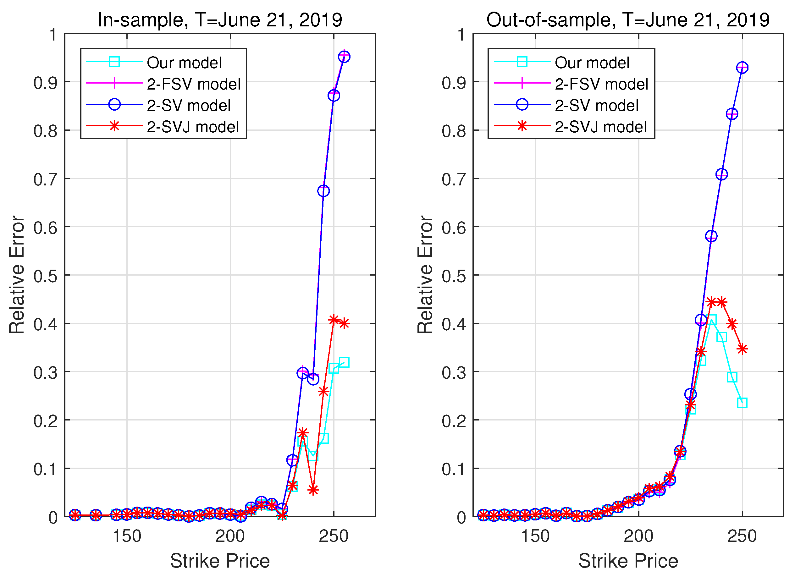
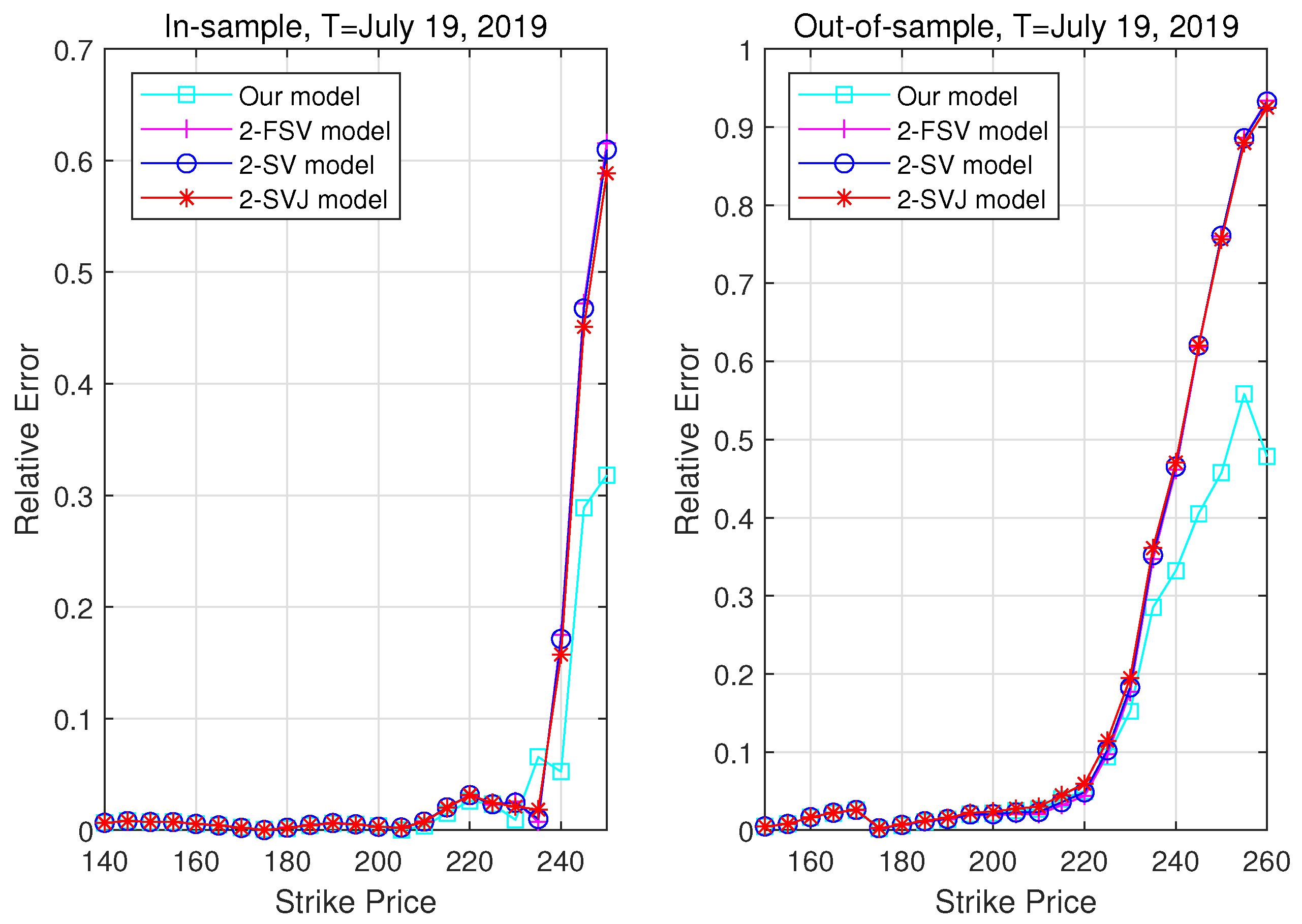
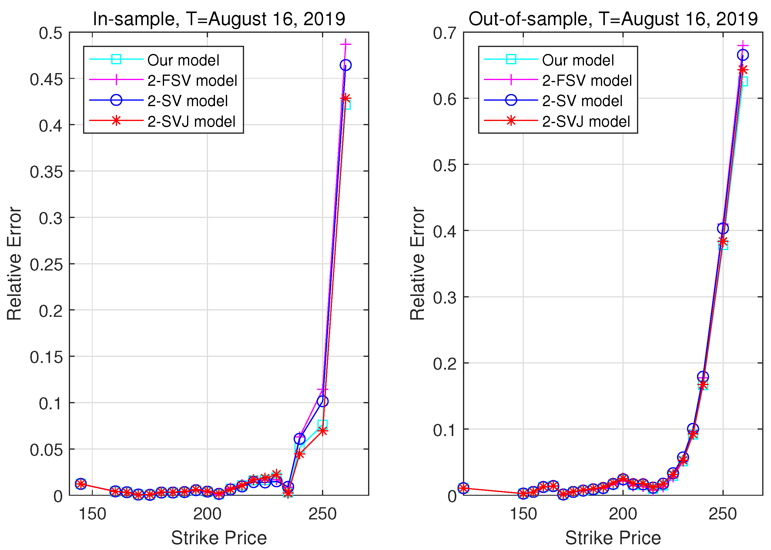
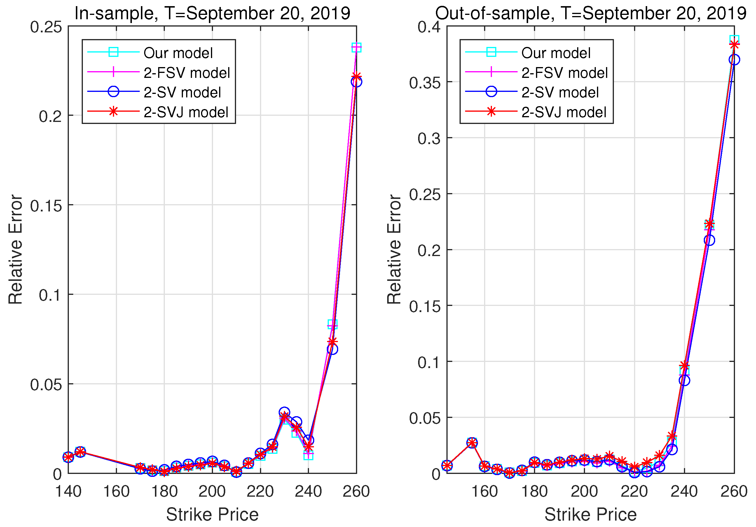
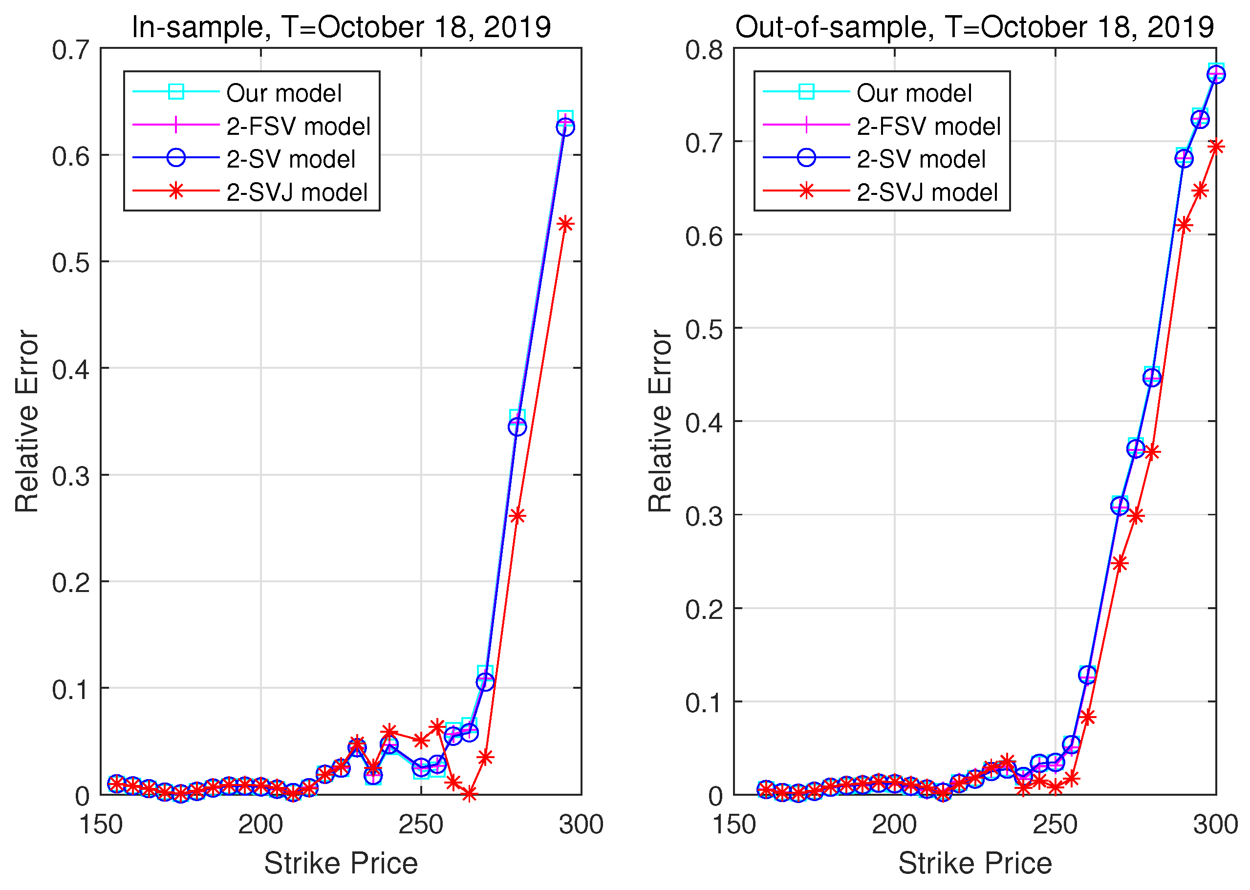
3.3. Pricing Performance
In this subsection, we present the empirical results for the calibrated models. In order to investigate the impacts of the systematic and idiosyncratic volatility and jump risks on equity option pricing, we took the 2-FSV, 2-SV, and 2-SVJ models as benchmark models to evaluate the pricing performance of our proposed model.
Figure 1, Figure 2, Figure 3, Figure 4, Figure 5, Figure 6, Figure 7, Figure 8, Figure 9 and Figure 10 exhibit the predicted prices of the four model specifications and market prices listed on 9 May 2019, with 11, 16, 21, 26, 31, 51, 71, 96, 116, and 181 trading days to expiry, respectively. Here, the predicted prices (out-of-sample pricing) were calculated by the in-sample calibration parameters reported in Table 1. One can clearly observe from the left panels of Figure 1, Figure 2, Figure 3, Figure 4, Figure 5, Figure 6, Figure 7, Figure 8, Figure 9 and Figure 10 that the option prices obtained by theoretical models were generally closer to the market prices for different strike prices. To further investigate the pricing performance of the four models, the right panels of Figure 1, Figure 2, Figure 3, Figure 4, Figure 5, Figure 6, Figure 7, Figure 8, Figure 9 and Figure 10 show the relative price differences (relative errors) between the theoretical model prices and market prices.5 For simplicity, we refer to a call option as deep out-of-the-money (DOTM) if ; out-of-the-money (OTM) if ; at-the-money (ATM) if ; in-the-money (ITM) if ; and deep in-the-money (ITM) if . Moreover, we considered options less than 60 days to expiration as short term; options with 60–120 days to expiration as medium term; and options larger than 120 days to expiration as long term. For the options with 11, 16, 21, 26, 31, and 51 trading days to expiry, the relative pricing errors produced by our proposed model were all significantly lower than those of 2-FSV, 2-SV, and 2-SVJ models in the case of DOTM options, while the relative errors of all models were slightly higher.
Figure 1.
The comparison of predicted prices of four model specifications and market prices on 9 May 2019, with maturity T = 24 May 2019.
Figure 2.
The comparison of predicted prices of four model specifications and market prices on 9 May 2019, with maturity T = 31 May 2019.
Figure 3.
The comparison of predicted prices of four model specifications and market prices on 9 May 2019, with maturity T = 7 June 2019.
Figure 4.
The comparison of predicted prices of four model specifications and market prices on 9 May 2019, with maturity T = 14 June 2019.
Figure 5.
The comparison of predicted prices of four model specifications and market prices on 9 May 2019, with maturity T = 21 June 2019.
Figure 6.
The comparison of predicted prices of four model specifications and market prices on 9 May 2019, with maturity T = 19 July 2019.
Figure 7.
The comparison of predicted prices of four model specifications and market prices on 9 May 2019, with maturity T = 16 August 2019.
Figure 8.
The comparison of predicted prices of four model specifications and market prices on 9 May 2019, with maturity T = 20 September 2019.
Figure 9.
The comparison of predicted prices of four model specifications and market prices on 9 May 2019, with maturity T = 18 October 2019.
Figure 10.
The comparison of predicted prices of four model specifications and market prices on 9 May 2019, with maturity T = 17 January 2019.
It is also worth noting that the pricing performance of the stochastic model with jump behavior was much better than that of the model without jump in the case of deep out-of-money. For the options with 71, 96, 116, and 181 trading days to expiry, we did not find the same conclusions as the above short term options. In conclusion, the pricing performance of equity option valuation model considering market and idiosyncratic volatility and jump risks was significantly improved for short term and DOTM options.
To summarize the model calibration results, we also adopted the RMSE as a measure of the goodness of fit. Table 2 reports the out-of-sample pricing errors for the four models across different maturities. Note from Table 2 that our proposed model generally outperformed the other three models in terms of out-of-sample pricing errors. In fact, the same was true for in-sample, whose pricing errors were generally lower than those of the out-of-sample. We will not repeat them here. To measure the extent to which a model was better or worse than another, we defined the improvement rate as the relative differences between the pricing errors from the benchmark model and our proposed model, i.e.,
where and denote the RMSE implied by our model and benchmark model, respectively. A positive (or negative) value of improvement rate meant that our model yielded lower (or higher) pricing errors than benchmark model, implying that the pricing performance of the former was better (or worse) than that of the latter by a percentage of that value.
Table 2.
Out-of-sample pricing errors. Note: This table shows the out-of-sample pricing errors across different maturities. Pricing errors are reported as the root mean squared errors (RMSE) of option prices for four models.
From the last column of Table 2, we can see that our model was superior to the 2-SVJ model across different maturities, which meant that it was necessary to consider the market factor structure in equity option pricing. From the third last column of Table 2, the improvement rate indicated that our model slightly outperformed the 2-FSV model in terms of short term options, but was worse than that of both medium and long term. In spite of this, our empirical study presented here could at least illustrate that the equity option pricing model considering systematic and idiosyncratic volatility and jump risks may offer a good competitor of the models of (), (), or () for some other equity option markets.
4. Conclusions
In (), the issues of the equity volatility levels, skews, and term structures were investigated by using equity option prices and the principal component analysis method. Their empirical results indicated that the equity options had a strong factor structure, and then, they developed an equity option pricing model with a CAPM factor structure and stochastic volatility. In addition, jumps in stock returns of individual firms were triggered by either systematic events or idiosyncratic shocks. Some recent studies indicated that idiosyncratic jumps were a key important determinant of expected stock; see, for example, (), () and ().
Motivated by these insights, we developed a novel model for pricing individual equity options that incorporated a market factor structure, which could be seen as a generalized version of the work by (). Specifically, in our model, the individual equity prices were driven by the market factor, as well as an idiosyncratic component that also had stochastic volatility and jump. Due to our model belonging to the affine class, we derived the closed-form solutions for the prices of both the market index and individual equity options by utilizing the Fourier inversion. In addition, we provided the empirical results to test the pricing performance of our proposed factor model based on the S&P 500 index and the AAPL stock on options. Toward this end, we empirically compared the pricing performance of our proposed model with those of the other three classical two factor stochastic volatility models being taken as benchmark models. The out-of-sample pricing performance of equity option valuation model considering market and idiosyncratic volatility and jump risks was significantly improved for short term and DOTM options. In conclusion, the empirical results presented here at least confirmed that the equity option pricing model considering systematic and idiosyncratic volatility and jump risks may offer as good competitor of the models of (), (), or () for some other option markets.
Funding
This work was supported by the National Natural Science Foundation of China (Grant No. 71901124) and the Natural Science Foundation of Jiangsu Province (Grant No. BK20190695).
Conflicts of Interest
The author declares no conflict of interest.
References
- Andersen, Torben G., Nicola Fusari, and Viktor Todorov. 2015. The risk premia embedded in index options. Journal of Financial Economics 117: 558–84. [Google Scholar] [CrossRef]
- Bakshi, Gurdip, Charles Cao, and Zhiwu Chen. 1997. Empirical performance of alternative option pricing models. Journal of Finance 52: 2003–49. [Google Scholar] [CrossRef]
- Bakshi, Gurdip, Nikunj Kapadia, and Dilip Madan. 2003. Stock return characteristics, skew laws, and the differential pricing of individual equity options. Review of Financial Studies 16: 101–43. [Google Scholar] [CrossRef]
- Bakshi, Gurdip, and Nikunj Kapadia. 2003a. Delta-hedged gains and the negative market volatility risk premium. Review of Financial Studies 16: 527–66. [Google Scholar] [CrossRef]
- Bakshi, Gurdip, and Nikunj Kapadia. 2003b. Volatility risk premiums embedded in individual equity options: Some new insights. Journal of Derivatives 11: 45–54. [Google Scholar] [CrossRef]
- Bardgett, Chris, Elise Gourier, and Markus Leippold. 2019. Inferring volatility dynamics and risk premia from the S&P 500 and VIX markets. Journal of Financial Economics 131: 593–618. [Google Scholar]
- Bates, David S. 1996. Jumps and stochastic volatility: Exchange rate processes implicit in Deutsche mark options. Review of Financial Studies 9: 69–107. [Google Scholar] [CrossRef]
- Bates, David S. 2000. Post-’87 crash fears in the S&P 500 futures option market. Journal of Econometrics 94: 181–238. [Google Scholar]
- Broadie, Mark, Mikhail Chernov, and Michael Johannes. 2007. Model specification and risk premia: Evidence from futures options. Journal of Finance 62: 1453–90. [Google Scholar] [CrossRef]
- Bégin, Jean-François, Christian Dorion, and Geneviève Gauthier. 2020. Idiosyncratic jump risk matters: Evidence from equity returns and options. Review of Financial Studies 33: 155–211. [Google Scholar] [CrossRef]
- Carr, Peter, and Dilip B. Madan. 2012. Factor models for option pricing. Asia-Pacific Financial Markets 19: 319–29. [Google Scholar] [CrossRef]
- Cheang, Gerald H. L., Carl Chiarella, and Andrew Ziogas. 2013. The representation of American options prices under stochastic volatility and jump-diffusion dynamics. Quantitative Finance 13: 241–53. [Google Scholar] [CrossRef]
- Cheang, Gerald H. L., and Len Patrick Dominic M. Garces. 2019. Representation of exchange option prices under stochastic volatility jump-diffusion dynamics. Quantitative Finance. [Google Scholar] [CrossRef]
- Christoffersen, Peter, Kris Jacobs, and Chayawat Ornthanalai. 2012. Dynamic jump intensities and risk premiums: Evidence from S&P 500 returns and options. Journal of Financial Economics 106: 447–72. [Google Scholar]
- Christoffersen, Peter, Mathieu Fournier, and Kris Jacobs. 2018. The factor structure in equity options. Review of Financial Studies 31: 595–637. [Google Scholar] [CrossRef]
- Christoffersen, Peter, Steven Heston, and Kris Jacobs. 2009. The shape and term structure of the index option smirk: Why multifactor stochastic volatility models work so well. Management Science 55: 1914–32. [Google Scholar] [CrossRef]
- Duffie, Darrell, Jun Pan, and Kenneth Singleton. 2000. Transform analysis and asset pricing for affine jump diffusions. Econometrica 68: 1343–76. [Google Scholar] [CrossRef]
- Eraker, Biørn, Miichael Johannes, and Nicholas Polson. 2003. The Impact of Jumps in Volatility and Returns. Journal of Finance 58: 1269–1300. [Google Scholar] [CrossRef]
- Fouque, Jean-Pierre, and Adam P. Tashman. 2012. Option pricing under a stressed-beta model. Annals of Finance 8: 183–203. [Google Scholar] [CrossRef]
- Fouque, Jean-Pierre, and Eli Kollman. 2011. Calibration of stock betas from skews of implied volatilities. Applied Mathematical Finance 18: 119–37. [Google Scholar] [CrossRef]
- Kapadia, Nishad, and Morad Zekhnini. 2019. Do idiosyncratic jumps matter? Journal of Financial Economics 131: 666–92. [Google Scholar] [CrossRef]
- Kou, Steven G. 2002. A jump-diffusion model for option pricing. Management Science 48: 1086–101. [Google Scholar] [CrossRef]
- Merton, Robert C. 1976. Option pricing when underlying stock returns are discontinuous. Journal of Financial Economics 3: 125–44. [Google Scholar] [CrossRef]
- Wong, Hoi Ying, Edwin Kwan Hung Cheung, and Shiu Fung Wong. 2012. Lévy betas: Static hedging with index futures. Journal of Futures Markets 32: 1034–59. [Google Scholar] [CrossRef]
- Xiao, Xiao, and Chen Zhou. 2018. The decomposition of jump risks in individual stock returns. Journal of Empirical Finance 47: 207–28. [Google Scholar] [CrossRef]
| 1. | In fact, the work of () is a complement to the recent studies that disentangle the four types of risks in equity premiums, such as (), who developed a GARCH-jump model in which an individual firm’s systematic and idiosyncratic risk have both a Gaussian diffusive and a jump component. Their empirical results showed that normal diffusive and jump risks have drastically different effects on the expected return of individual stocks by using 20 years of returns and options on the S&P 500 and 260 stocks. |
| 2. | One can refer to Assumption 2.1 of () and () for a more detailed explanation. |
| 3. | Obviously, our proposed model for the dynamics of the market factor and individual equity prices is an extension of (). In fact, our model also can be regarded as a further generalization of () and () by taking into account the factor structure. |
| 4. | One can refer to the Assumption 2.1 of () and () for a more detailed explanation. |
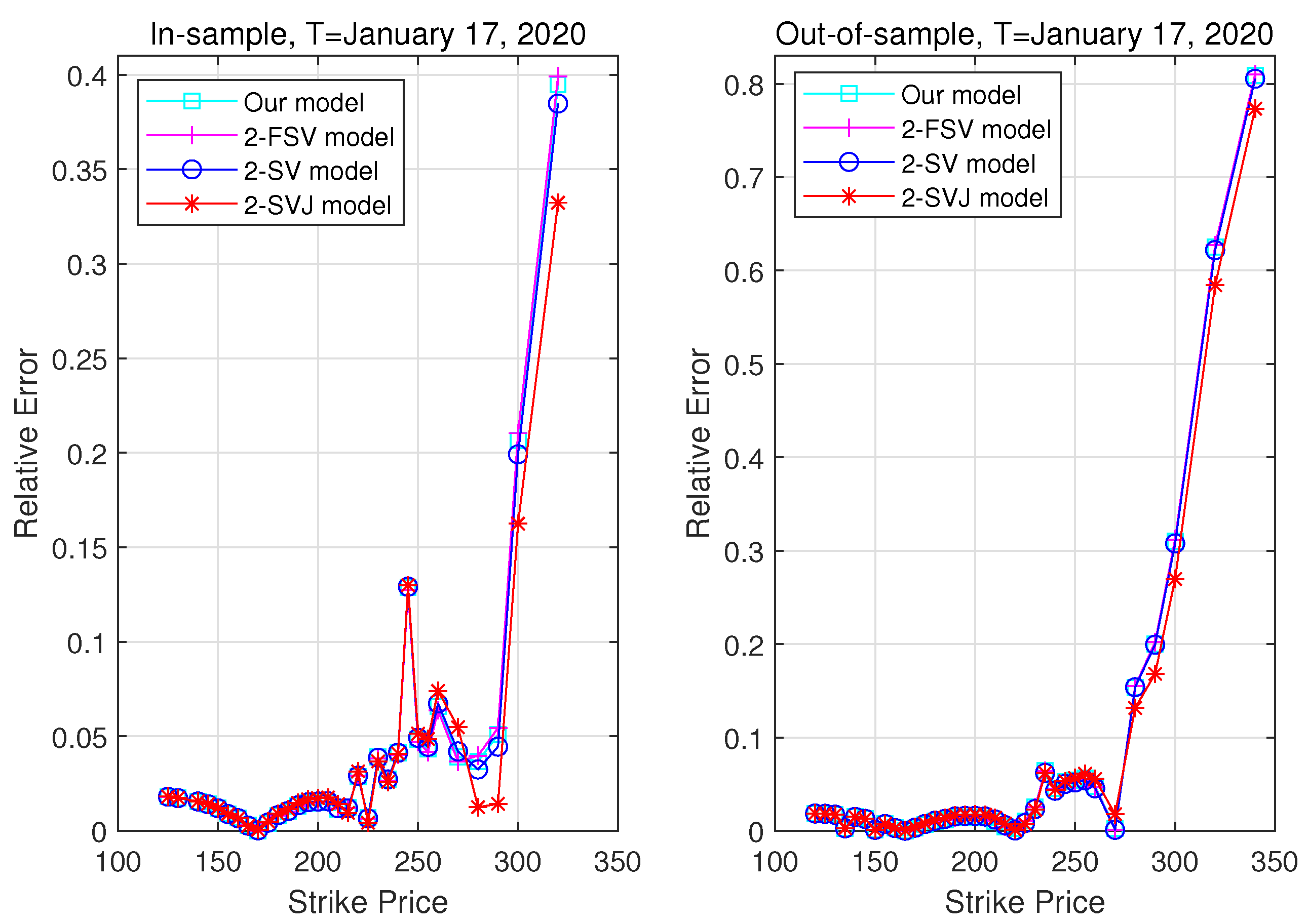
| 5. | The relative error is defined by , where and denote the theoretical model option prices and the real market prices, respectively. |
© 2020 by the author. Licensee MDPI, Basel, Switzerland. This article is an open access article distributed under the terms and conditions of the Creative Commons Attribution (CC BY) license (http://creativecommons.org/licenses/by/4.0/).