Understanding Forest Health with Remote Sensing-Part II—A Review of Approaches and Data Models

Abstract

Stress in forest ecosystems (FES) occurs as a result of land-use intensification, disturbances, resource limitations or unsustainable management, causing changes in forest health (FH) at various scales from the local to the global scale. Reactions to such stress depend on the phylogeny of forest species or communities and the characteristics of their impacting drivers and processes. There are many approaches to monitor indicators of FH using in-situ forest inventory and experimental studies, but they are generally limited to sample points or small areas, as well as being time- and labour-intensive. Long-term monitoring based on forest inventories provides valuable information about changes and trends of FH. However, abrupt short-term changes cannot sufficiently be assessed through in-situ forest inventories as they usually have repetition periods of multiple years. Furthermore, numerous FH indicators monitored in in-situ surveys are based on expert judgement. Remote sensing (RS) technologies offer means to monitor FH indicators in an effective, repetitive and comparative way. This paper reviews techniques that are currently used for monitoring, including close-range RS, airborne and satellite approaches. The implementation of optical, RADAR and LiDAR RS-techniques to assess spectral traits/spectral trait variations (ST/STV) is described in detail. We found that ST/STV can be used to record indicators of FH based on RS. Therefore, the ST/STV approach provides a framework to develop a standardized monitoring concept for FH indicators using RS techniques that is applicable to future monitoring programs. It is only through linking in-situ and RS approaches that we will be able to improve our understanding of the relationship between stressors, and the associated spectral responses in order to develop robust FH indicators.

1. Introduction

There is a growing awareness of the multitude of ecosystem services that forests provide and their importance for the wellbeing of humans and conservation of the environment. Forest ecosystems (FES) are well known as hosts of biodiversity, carbon and oxygen pools, sources of timber, water purification systems and providers of livelihoods, and yet an increasing number of anthropogenic threats endanger FES. While direct stressors are a result of forest utilization or land use changes, indirect stress is caused by drivers such as climate change, air pollution and globalization, which in turn may bring about an additional impact from invasive species [1].

Due to the crucial importance of forests, it is of high relevance to better understand how different stressors affect forest conditions and how these mechanisms interact with the type, structure and history of the forest. It is only then that forest management and conservation strategies can be adapted to maintain and improve forest health (FH) and to cope with new and upcoming threats. For both, it is important to develop monitoring techniques, which provide information on the past and present state of FH. Such information forms the basis for research on the interactions between forest conditions and stressors. This is particularly relevant and urgent for FES where growth and regeneration can take centuries. Thus, today’s management decisions will determine the shape of our forests for future generations. To monitor and understand the complexity of FH, its entities, drivers, functional mechanisms and impacts, it is imperative to develop effective standardized large scale long-term monitoring systems.

FH monitoring (FHM) has a long history and is carried out by private forest owners, forest administrations and other public entities at local, national and international levels. There are numerous in-situ monitoring programs at the local and regional scales that increasingly utilize standardized indicators of FH. Among the largest monitoring programs are the FOREST EUROPE program of the European Union and the International Co-operative Programme on Assessment and Monitoring of Air Pollution Effects on Forests (EU/ICP Forests) which started in 1990 [2], the FHM program of the United States [3] and the Chinese national program on ecological functions [4]. While in some countries, FHM belongs to independent monitoring programs, other countries include the assessment of FH in their national forest inventories [5]. Table 1 provides an overview on current long-term FHM monitoring programs that use in-situ methods.

Table 1. Long-term monitoring of forest health (FH) at country, European and global level.

Level/Scale	Responsible Body	Description	Resources/Links
Country level: Germany	Johann Heinrich von Thünen-Institute	Forest condition monitoring (FCM).	[6]
		Level-I-Monitoring.
		Frequency: Annual.
		Compilation of national reports on forest conditions for Germany (FCA). FH assessed using systematic sample grid of permanent plots.
	Federal Research Institute for countryside, forests and fisheries	Intensive monitoring.
		Level-II Monitoring.
		Frequency: Continuous.
		66 sites intensively monitored, partly through continual sampling of relevant ecosystem compartments in selected FES.
	Federal Ministry for Food and Agriculture	National forest inventory.	[7]
		Level-III-Monitoring.
		Frequency: Every 10 years.
		Status and development of the forests of Germany derived from a sample based large scale forest inventory.
Country level: USA	United States Department of Agriculture(USDA) Forest Service	FH Monitoring (M).	[8]
		Frequency: Annual.
		National program designed to determine the status, changes, and trends in indicators of forest condition on an annual basis.
Country level: Canada	Canadian Forest Service (CFS)	National FHM Network.	[9]
		Frequency: 5-years.
		Established 1994 based on earlier Acid Rain Monitoring Network. Plot-based Bi-annual to 5-year repetition depending on the variables.
	National Forest Inventory (NFI), Canada	National Forest Inventory.	[10]
		Frequency: 10-years.
		Mixed plot and RS based. Includes inventory parameters + assessment of insect, disease, fire and other disturbance damage.
European level	United Nations Economic Commission for Europe (UNECE)	ICP.	[11]
		Frequency: Annual.
		International Co-operative Programme on the Assessment and Monitoring of Air Pollution Effects on Forest. Developed to standardise the recording of different FH indicators on three levels of intensity.
Global level	Food and Agriculture Organization of the United Nations (FAO)	Forest Resources Assessment.	[12]
		Frequency: 5-years.
		FH recorded by the FAO as part of the Forest Resources Assessment (FRA). Individual countries report their findings to the FAO, which then compiles a report.

FH as such cannot be observed or monitored directly but needs to be assessed using indicators which are then combined to create a holistic picture of the forest condition. Different initiatives and programs have developed FH indicators. For example, FHM conducted by the US Forest Service collects variables on lichen communities, forest soils, tree crown conditions, vegetation diversity and structure, downed woody materials and ozone damage [13]. The FOREST EUROPE program defines 7 criteria to describe the status of European forests, where criterion 3 analyses the “Maintenance of Forest Ecosystem Health and Vitality” [2]. Both programs use sample based in-situ assessments, where the set of indicators is either directly observed (e.g., amount of deadwood, species composition) or quantified by expert judgement (e.g., defoliation and discoloration classes). The quality and consistency of such assessments depend on the expertise of the field teams, which can limit comparability between assessments. Thus, for various important FH indicators such as tree crown density, defoliation, “naturalness” or regeneration potential, there are still no standardized metrics nor direct measuring procedures available. However, these in-situ FH assessments are regularly conducted and have proven to be useful to detect changes in FH conditions over longer periods. Remote sensing (RS) techniques are regularly used for forest monitoring. However, in the context of operational national and international FHM programs, RS currently only plays a minor role. To provide but one example: in the 364-page report for 46 European countries, the term “remote sensing” occurs only once where it is stated that RS and geographic information systems are new technologies that will be used by some countries [2]. Pause et al. [14] concluded that a major advantage of implementing remote-sensing techniques is the possibility of repeatedly acquiring standardized information over large areas at low costs with high frequency. However, RS techniques are only helpful to improve the objectivity of FHM when they can be reliably linked to FH indicators. Furthermore, a combined terrestrial and remote-sensing monitoring system not only serves to monitor changes in forest conditions, but also to relate the changes to the drivers [15].

In the first part of this paper series, Lausch et al. [16] provided a working definition of FH and reviewed FH indicators, as well as their importance and relevance for the development of FHM programs. They introduced the concept of Spectral Traits (ST) and spectral trait variations (STV) as a framework for FHM. In this second paper, we review existing remote-sensing systems and evaluate their potential for monitoring specific FH indicators. This paper addresses the following questions:

• Which factors are important when designing FHM programs that combine terrestrial and remote-sensing data?
• Which remote sensors and systems are suitable for monitoring which FH indicators?
• Which new technologies and current developments are relevant for the design of future FHM programs?

In the introduction, we provide an overview of the current close-range FHM programs to identify potential links between in situ observations and RS data. Section 2 reviews the trends and new technologies for close-range RS approaches. Section 3 analyses air- and space-borne RS systems for estimating and monitoring FH indicators. In Section 4, we describe approaches of physical and empirical models followed by conclusions in Section 5.

2. Trends in Close-Range RS Approaches for Assessing FH

Traits and trait variations in FES display specific spectral responses in RS data that are caused by the taxonomy, phenology and phylogenetics of forest species and communities as well as by natural and anthropogenic stressors [16,17]. The spectrum of responses ranges from additive reinforcing effects to contrary effects, reductive or even exclusive signals. To correctly interpret these spectral response signals in terms of disturbance or stress, as well as to gain sufficient information for calibrating and validating airborne and space-borne RS data, extensive close-range RS measurements (Figure 1, Table 2) as well as physically-based models (Section 5) are needed.

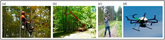
Figure 1. Methods and materials for sampling canopy materials in forest, (a) Tree climbers, photo by Michael Lender; (b) Cherry picker, photo by Franz Baierl; (c) Crossbow, photos by Zhihui Wang and; (d) Unmanned Aerial Vehicle (UAV).

Table 2. Technical and methodological options for close-range RS to observe FH indicators.

Close-Range Measurement Approaches/References	Advantages/Applications	Disadvantages
Field Spectrometers [21,22,23,24]	Basis for research on spectral characteristics of biochemical-biophysical, morphological traits. Spectral databases for classification and validation. Basis for research on taxonomic, phylogenetic, genetic, epigenetic or morphological-functional features.	Analysis at molecular level. Geometric, structural, distribution, population and community effects are not measurable. No standardized measurement protocols available
Spectral laboratory (Manual operation) [18,25,26,27,28,29].	Seasonal, annual, long-term. Biochemical-biophysical, structural variables in organs (roots, leaf, stem) and whole tree. Experimental stress analyses (drought, heavy metals, tropospheric ozone, flooding, nitrogen loads, etc.). Extensive lab-based measurement program for biotic, abiotic, climate conditions. Comparative analyses can be conducted under natural or artificial conditions. Multi-sensor recording at specific plant development stages. Storage in spectral databases for validation and calibration.	Development of measuring boxes for the sensors (automated). Age and development stages of the trees are a limiting factor (often only trees up to 5 years old can be recorded)
Plant phenomics facilities (Fully automatic operation), Ecotrons (Controlled environmental facility), [30,31,32,33,34,35,36,37,38,39,40,41,42,43,44,45,46,47,48].
Tower (eddy flux tower) with different non-invasive measuring technologies as well as RS technology (mobile, permanently installed), [49,50,51,52].	Long-term monitoring. International networks exist. Extensive multi sensor monitoring is possible for biotic and abiotic conditions (e.g., phenocams). Spectral measurements directly on canopy level.	Local results for a particular site, not transferable
Wireless sensor networks (WSN) [53,54,55,56,57,58,59,60,61,62]	Long-term high frequency monitoring. Extensive multi sensor measurement is possible. Measuring various biochemical-biophysical, structural variables in organs (roots, leaf, stem) and whole tree. Enables results over more extensive areas. Easy to install in remote areas.	Primarily non-imaging sensor technology can be implemented

In-situ sampling of forest canopy elements for measurement of leaf properties such as chlorophyll, protein, water content, leaf area index (LAI) or functional plant traits such as photosynthesis activity is difficult compared to sampling of ground vegetation. Recording this kind of information often requires tree climbers, lifting platforms or towers, Unmanned Arial Vehicle (UAV) with arms for cutting small branches or rifles or harpoons to shoot down leaf material (Figure 1).

In addition to UAVs, aircrafts and space-borne RS applications, close-range RS approaches are increasingly being established to support the observation of FH indicators as shown in Figure 2. They range from spectral analyses of forest species to terrestrial wireless sensor networks as summarized in Figure 2 and Table 2.

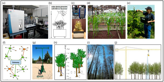
Figure 2. Overview of different close-range RS methods to analyse indicators of FH, (a) Laboratory spectrometer; (b,c) Ash trees monitored in a close-range RS spectral laboratory (manual) with imaging hyperspectral sensors AISA EAGLE/HAWK (modified after Brosinksy et al. [18]; (d) Automated plant phenomics facilities (e) Field-spectrometer measurements; (f) Wireless sensor networks—WSN; (g) One sensor node of the WSN (graphic, photo (f,g)) by Jan Bumberger and Hannes Mollenhauer); (h) instrumentation of the Hohes Holz forest site (modified by Wöllschläger et al. [19] (i) tower with different RS instruments, (j) mobile crane with RS measurement platform (modified after Clasen et al. [20]).

2.1. Close-Range RS Approaches—Spectral Laboratory, Plant Phenomics Facilities and Ecotrons

Close-range investigations are conducted to determine the spectral responses of FH traits and to derive meaningful models from them (see Table 2). Reactions of woody plants to stress are species specific [59,63]. Teodoro et al. [59] analysed different strategies of Brazilian forest tree species to cope with drought stress and maintain plant functioning. As reactions of woody plants to stress factors like drought can often only be observed years later in the form of biochemical, physiological or geometrical changes to woody plant traits [27], the ability of different tree species to adapt to climate change is still not well understood [64].

With the help of close-range RS approaches, extensive long-term stress monitoring can be carried out that takes into account vegetation phenological cycles as well as inter-annual variations. To specifically investigate different stress factors, experimental settings are best suited as they provide reliable input for models and eliminate confounding factors. Brosinsky et al. [18] investigated the spectral response of ash trees (Fraxinus excelsior L.) to physiological stress from flooding over a 3-month period, whereas Buddenbaum et al. [27] modelled the photosynthesis rate of young European beech trees under drought stress following a two-year water stress treatment by using close-range hyperspectral visible, near infrared and thermal sensors. Another common method to induce water stress is the girdling of trees with differing degrees of intensity [65,66].

The Genotype comprises hereditary information about the DNA of a species while the phenotype represents the physiological, morphological, anatomical, development characteristics and the interactions of species with their environmental conditions, resource limitations and stress factors. Insights into genotype and phenotype interactions in plant stress physiology are not only gained from recording individual plant ST, but also by including the entire genotype-epigenetic-phenotypic-environment matrix [67]. This can be achieved, for example, by recording phenotypical plant traits in plant phenomic facilities [30,34] or controlled environmental facilities—Ecotron [38]. The acquisition of phenotype plant traits in plant phenomics facilities has so far mainly been carried out for crop vegetation [33,34,68]. For woody plants, preliminary investigations have been restricted to fruit trees [36]. Phenotypical investigation of woody plants should therefore be augmented in the future, in order to be able to better understand the mechanisms and stress factor interactions involved when interpreting FH indicators observed using RS. It is these kinds of comparisons that support research on the effects of the Bidirectional Reflectance Distribution Function (BRDF), scale and different RS platforms as well as different sensor characteristics on model design [69].

The regulation of photosynthetic electron transport, as well as its feedback processes and the assessment of photosynthetic efficiency and stress in crops, grassland and forest canopies, have been investigated with sun-induced chlorophyll fluorescence methods at leaf [41], field, and regional levels [42,43,44,45]. Spectroscopic techniques for the detection of chlorophyll fluorescence forms the basis for the European Space Agency (ESA) Fluorescence Explorer Sensors (FLEX, [45,46,70]) to be launched in 2018. With its very high spectral resolution across the 0.3–3.0 μm range, FLEX will be the first satellite that is able to directly measure solar-induced chlorophyll fluorescence and thus forest stress indicators and other vegetation parameters.

Disadvantages of close-range RS laboratory methods include the use of artificial light sources and the short distance between the sensor and object. Substantial image pre-processing and calibration is often required to compare lab and field measurements. However, given the experimental setting, BRDF effects can be observed with high sensitivity and the spatial resolutions are much finer (mm) than with airborne- and space-borne RS. Thus, experimental spectral laboratories allow continuous investigation of phenotypical features as well as a comprehensive understanding of the spectral response to stress-physiological parameters in forest vegetation. Table 3 summarizes findings from exemplary close-range RS studies of FH that illustrate the points made above.

Table 3. Example studies illustrating the use of spectral laboratory, plant phenomics and controlled environmental facilities in common FH applications.

Application	Example Studies	Main Findings
Genotype-epigenetic and phenotype interactions	[30,34]	Qualitative, quantitative and spectroscopic recording of plant species phenotypes for better understanding of the link between the genotype and the phenotype.
	[67]	Understanding the impacts and resilience to stress, disturbance or resourcelimitations of forest species and ecosystems is crucial for understanding the genotype-epigenetic-phenotypic-environment matrix.
Goal of the Plant Phenotyping Network	[32,71]	International Plant Phenotyping Network [72]: (1) Innovative non-invasive techniques such as stereo systems, hyperspectral, RGB, thermal, fluorescence cameras, laser scanners or X-ray tomography; (2) Continuous, very high temporal resolution acquisition of phenotypical traits that provides important reference information for RS approaches; (3) ST/STV are saved in databases; (4) Data can be used for calibration and validation of air- and spaceborne RS data.
Spectral traits of leaves	[27]	Laboratory-based imaging spectroscopy combined with the inversion of a radiative transfer model is able to derive biochemical spectral traits (N, chlorophyll content, carotenoids, brown pigments, water content, dry mass) at the leaf level on the sub-millimeter scale.
Development and testing of new close-range RS technologies	[41,42,43,44,45]	Investigations of sun-induced chlorophyll fluorescence methods at the leaf level, field level, and the regional level are only possible through fundamental research in Plant Phenomics Facilities and Ecotrons.
	[46,47,48]	Evaluated the effects of different plant stresses on photosynthetic performance. This research on chlorophyll fluorescence and its acquisition using spectroscopic techniques forms the basis for developing the European Space Agency (ESA) Fluorescence Explorer Sensors (FLEX, [45,46,70]).
	[47]	Development of 3-D digital imaging and a portable terrestrial laser scanner for detecting seasonal change within broad-leaved forest.
	[73]	Development of a canopy leaf area density profile.
	[48]	3D-imaging techniques for monitoring the spatio-temporal effects of herbicides on plants.
Monitoring of stress to woody plants	[27]	Reactions to stress factors like drought, can often only be observed years later in the form of biochemical, physiological or geometrical changes to woody plant traits (e.g., in tree rings observed from cross cuttings). Age and development stages of the trees are a limiting factor (often only trees up to the age of 5 years can be recorded).

2.2. Close-Range RS Approaches—Towers

In order to upscale findings from experimental laboratory settings, which are often for leaf scale analysis, close-range RS can be implemented using mobile towers [20] or permanently installed towers [49] equipped with RS sensors to analyze spectral effects on the canopy level. (Table 4, Figure 2). Such systems may include automated digital time-lapse cameras (e.g., phenocams [51]), multispectral and thermal sensors, and non-imaging spectral sensors to monitor the status and changes of FH indicators over long periods of time at regular intervals. The US National Ecological Observatory Network (NEON) and the European Union’s Integrated Carbon Observation System (ICOS) are continental-scale ecological research networks that promote the international implementation, use, standardization as well as analysis of phenocam data [51].

Table 4. Example studies illustrating the use of towers with different RS technology (mobile, permanently installed) in common applications.

Application	Example Studies	Main Findings
Phenocam networks	[51]	US National Ecological Observatory Network (NEON) and the European Union’s Integrated Carbon Observation System (ICOS).
		Fully-automated digital time-lapse cameras (phenocams) and other cameras can be easily mounted on towers. They are crucial sensors for recording, quantifying, monitoring and understanding of phenological traits and the interactions of ST/STV relations to stress, disturbances and resource limitations in forest ecosystems.
Individual towers	[52]	Fully automated spectral data recording system for phyto-pigments (chlorophyll, carotenoids, anthocyanins) under different view and sun angles. Used to assess diurnal and seasonal variations of plant physiological processes under different illumination and weather conditions. High spatial resolution allows measurement of spectral response of individual tree crowns. Systematic recording of ST/STV can be linked to eddy covariance gas exchange measurements.
Flux tower networks	[49,50]	Linking flux towers in an international network (FLUXNET, [76]). Flux towers generally include integrated sampling of ecosystem parameters such as carbon dioxide, water vapour and energy fluxes, as they cycle through the atmosphere, vegetation and soil. FLUX towers are often coupled with the sensor technologies such as spectrometers or soil sensors.
Spectral networks	[77]	Spectral network (SpecNet, [78]). Multi-scale spectral RS from satellites, aircraft, UAVs, mobile tram systems, portable spectrometers over same area as flux measurements. The goals of SpecNet are: (1) Monitoring surface–atmosphere fluxes of water, carbon and vapor; (2) Understanding and assessing the impacts of disturbance and dynamic events (e.g., fire, extreme weather events, climate, land-use change).

Flux towers generally include integrated sampling of different ecosystem variables such as carbon dioxide, water vapour and energy fluxes. They are often coupled with sensor technologies such as spectrometers or soil sensors. Such combinations allow continuous measurements of vegetation productivity and environmental variables such as fluxes, soil moisture, and evapotranspiration, which can be assessed in relation to FH attributes. Permanently installed towers acquire individual point information but are of particular importance in terms of long-term measurements for the calibration and validation of airborne and space-borne RS data. Linking flux tower systems in an international network (FLUXNET, [50]) supports a better understanding of ecological processes and changes in FH using RS [74,75].

2.3. Close-Range RS Approaches—Wireless Sensor Networks (WSN)

Wireless sensor networks (WSN) consist of a potentially large set of sensors that communicate with each other based on wireless communication channels and standardized protocols. They can collect data on various environmental variables which can be used to describe complex ecosystem forest processes continually in a non-invasive, cost-effective, automated and real-time manner [53,79,80,81]. The design of the network, e.g., the spatial separation of the network nodes (sensor nodes), depends on the spatial variability of the environmental variables and ranges from centimetres to a maximum of about 1km depending on the wireless communication technology used.

In the context of FHM, WSNs are implemented for the detection and verification of forest fires in real time [53,55]. Brum et al. [60] used WSNs to demonstrate the effects of the 2015 El-Niño extreme drought on the sap flow of trees in eastern Amazonia. Oliveira et al. [58] used WSNs to record important processes of soil-plant-atmosphere interactions in tropical montane cloud forests in Brazil. They investigated how key forest ecosystem processes such as transpiration, carbon uptake and storage, and water stripping from clouds are affected by climatic variation and the temporal and spatial forest structure. Moreover, Teodoro et al. [59] and Oliveira et al. [58] used WSNs to demonstrate the interplay between hydraulic traits, growth performance and the stomata regulation capacity in three shrub species in a tropical montane scrubland of Brazil under contrasting water availability. The results showed that forest plant species employ different strategies in the regulation of hydraulic and stomatal conductivity during drought stress and thus substantiate the need for setting up WSN for different forest tree species and communities [59] (see Table 5). Innovative developments, ongoing miniaturisation, the cost-effective production of different non-invasive environmental sensors [61,62] as well as the latest data analysis and network technologies (e.g., semantics [82] and Linked Open Data (LOD, [83]) are all promising factors that promote the implementation of WSN as part of FHM programs.

Table 5. Example studies illustrating the use of wireless sensor networks (WSN) in applications.

Application	Example Studies	Main Findings
Forest fire detection	[53,55]	WSNs are implemented for the detection and verification of forest fires in real time.
Drought stress	[60]	WSNs used to demonstrate the effects of the 2015 El-Niño extreme drought on the sap flow of trees in eastern Amazonia.
Understanding physiological and ecological processes	[58]	Useful in recording and understanding important processes of soil-plant-atmosphere interactions in tropical montane cloud forests in Brazil, key forest ecosystem processes such as transpiration, carbon uptake and storage, and water stripping from clouds that are affected by climatic variation and the temporal and spatial forest structure.
	[59]	Important in monitoring and understanding hydraulic traits, growth performance and the stomata regulation capacity in three shrub species in a tropical montane scrubland of Brazil under contrasting water availability. The results showed that forest plant species employ different strategies in the regulation of hydraulic and stomatal conductivity during drought stress and thus substantiate the need for setting up WSN for different forest tree species and communities.

3. Trends in Air-and Space-Borne RS for Assessing FH

RS has advanced rapidly in recent years, including widespread adoption of LiDAR, RADAR, hyperspectral and integrated systems for a variety of forest applications. This section reviews these sensors types and their applicability in analysis and monitoring.

3.1. Light Detection and Ranging (LiDAR)

LiDAR is an active RS technique, where short pulses of laser light are distributed from a scanning device across a wide area and their reflections from different objects are subsequently recorded by the sensor. The result is a set of 3D points, which represents the scanned surfaces from where the pulses were reflected. More detailed descriptions of LiDAR technology can be found in [84,85].

Nowadays, laser-based instruments are used on all kinds of RS platforms, including terrestrial, UAVs, the well established airborne LiDAR scanning and satellite-based laser-based instrument (e.g., Geoscience Laser Altimeter System (GLAS), [86]).

The primary characteristic that makes LiDAR well suited for applications to monitor FH is the potential to reconstruct 3D forest structures within and below the canopy, which cannot be provided by passive remote-sensing techniques [87]. Therefore, LiDAR RS is an important component when it comes to monitoring FH characteristics related to canopy and tree structure and it adds a further dimension to the properties of optical RS.

Based on the capabilities of data recording, it is possible to distinguish between discrete return systems and full waveform systems. At the onset of LiDAR development, the sensors were only able to record either the first or the last reflection of the LiDAR beam, which in FES is generally the top of the trees (first reflection) and the terrain (last reflection). With the more recently developed full waveform systems, the whole pathway of the LiDAR beam through the canopy can be detected and recorded [88]. Moreover, additional echo attributes such as amplitude and intensity of the return signal can be provided, which can support the classification process. As a result, the characterization of the canopy structure is much more detailed with full waveform data [89], so that important FH indicators such as forest height and understory cover can be estimated with a lower bias and higher consistency [90].

For FHM applications, LiDAR systems are generally used that have a beam footprint of less than one-meter diameter on the ground. These so-called small footprint systems are preferred, because they provide a good link between the LiDAR beam and the structural vegetation attributes that subtly change as a consequence of stress or damage, sometimes within individual trees. By comparison, large footprint systems have beam diameters with up to several tens of meters on the ground; e.g., the GLAS instrument mounted on the Ice, Cloud and Land Elevation Satellite ICESat Platform with a footprint of 38 m [91]. Such systems can be used to model broad forest structural attributes but can only detect significant and widespread changes in forest structural condition or health [92].

The most important environmental application of LiDAR is the precise mapping of terrain and surface/canopy elevations. Such digital terrain models (DTMs) or digital surface models (DSMs) can be useful in monitoring FH indicators such as changes in tree height resulting from damage or deviations in growth due to stress [93,94,95]. Recent studies show that it is even possible to detect objects located on the ground surface such as coarse woody debris [96,97]. Coarse woody debris is an important indicator of FH, because it provides habitat to a multitude of endangered plant and animal species and plays an important role in the forest carbon cycle [98,99].

Because of its characteristics, LiDAR is well suited for measuring forest biophysical parameters, such as tree dimensions and canopy properties. Two main approaches have been developed over recent years. The area-based approach is a straightforward methodology where the height distribution of the LiDAR beam reflections is analyzed for a given area [100]. In a first step, different “LiDAR metrics”, such as the maximum height or fractional cover are calculated for each area. In a second step, these metrics are set in relation to conventional ground measurements of FH indicators such as Above Ground Biomass (AGB) or stand density for model calibration. In a final step, the models are used to predict the selected FH indicators for large areas using square grid cells. Such analysis is generally conducted using a priori stratification of stand types and tree species. In the years that followed, this methodology was proven to be able to determine key biophysical forest variables on a larger scale. So far, this method has been shown to deliver a precision of 4%–8% for height, 6%–12% for mean stem diameter, 9%–12% for basal area, 17%–22% for stem density and 11%–14% for volume estimations of boreal forests [100,101,102,103]. Because of the high accuracy of estimation of important FH parameters the area-based approach was further developed and adopted to operational forest inventories in boreal forests of Scandinavia [104]. For the temperate zone similar accuracies have also been achieved, although the presence of more complex forest structures, especially a higher number of tree species and a higher amount of standing dead wood leads to less accurate estimations and requires more effort in stratification and ground measurement to obtain species-specific results [105,106,107].

The second methodology is the individual tree approach, which has the objective of extracting single trees and modeling their properties. The procedure consists of four steps: (1) delineation of individual trees; (2) extraction of tree parameters such as height, species and crown parameters; (3) model calibration of the biophysical parameters: Diameter at Breast Height (DBH), volume and biomass with the help of reference trees measured on the ground; and finally (4) the application of models to predict DBH, volume and biomass for all delineated LiDAR trees. Based on the crown representations basic attributes reflecting tree health such as total volume, crown length, crown area and crown base height can be derived [108,109]. The extracted individual trees also form the basis for identifying the tree species. Within the 2D or 3D representation of the individual tree point cloud and waveform features are calculated and with the help of classification techniques, tree species can be determined [90,110]. While the differentiation between deciduous and coniferous trees can be performed with a high accuracy (>80%, up to ~97%) the differentiation within these classes is more difficult and leads to a higher classification error [111]. Moreover, it is possible to distinguish between living trees, standing dead trees and snags [112,113,114] or to map dead trees on the plot or stand level [115,116]. However, 3D LiDAR has its limitations for differentiating between trees species and dead trees unless it is not combined with multi- and hyperspectral optical data. One drawback of the single tree approach is that the LiDAR beam loses some signal strength on its way through the canopy. This results in an underestimation of individual trees in the understory [117]. To overcome this problem, methods have been developed to predict stem diameter distributions of forest stands based on the detectable trees in the upper canopy and LiDAR derived information about the vertical forest structure and density [118].

Besides the traditional parameters related to forest inventory, a multitude of FH parameters describing the ecological conditions of the forest can be estimated with LiDAR sensors. One key element to assess FH is the canopy cover which is defined as the projection of the tree crowns onto the ground divided by ground surface area [119]. This parameter can be easily translated to LiDAR data by dividing the number of returns measured above a certain height threshold by the total number of returns. Many studies have shown a strong (R² > 0.7) relationship between this LiDAR-metric and ground measurements [120]. By using hemispherical images or LAI-2000 sensor data for calibration, LAI and solar radiation can also be derived from LiDAR data with a high precision over large areas [108,121].

The vertical forest structure is of high relevance for the description of forest heterogeneity and for biodiversity assessments [122,123]. A widely used LiDAR metric to represent vertical canopy complexity is the coefficient of variation. Higher values correspond to more diverse multi-layer stands, while low values represent single layer stands [124]. The coefficient of variation can be applied to the point clouds, the digital crown model or individual trees. Zimble et al. [125] applied this principle and classified forest stands according to stand structure with LiDAR data and achieved an overall accuracy of 97%. Another approach is the partitioning of the vertical structure into different height layers in relation to ecological importance. Latifi et al. [107] divided the canopy into height layers according to phytosociological standards and found a strong relationship with different LiDAR metrics using regression models. Similar approaches were used by Vogler et al. [126] and Ewald et al, [127] to represent the understory relevant for birds and deer and to detect forest regeneration [128]. A more recent study applied a 3D segmentation algorithm to estimate regeneration cover and achieved an accuracy of 70% [129]. LiDAR-derived information about the vertical structure is also used for the assessment of forest fuels and their vertical distribution, which are important input variables in forest fire models supporting fire management [130,131].

As a result, LiDAR-RS is a powerful tool for monitoring FH indicators. It delivers detailed and accurate information about forest properties down to the scale of the individual tree. Nowadays, LiDAR is widely applied in RS research as a reference to test the accuracy of other methods as well as in practical forest inventories in the boreal zone of Scandinavia [102]. The development of new sensors will lead to multi- or hyperspectral LiDAR technology, which will combine the advantages of today’s LiDAR and optical sensors. These systems will be able to collect accurate 3D information and calibrated spectral information without facing the problems of varying illumination in the tree crowns. Furthermore, the resolution of the data will increase, enabling parameter extraction at the branch level [132].

Until now the application of LiDAR has been relatively costly because it is limited to airborne missions covering local to regional areas; currently there are no active space-borne missions providing data for mapping forest vegetation. The Global Ecosystem Dynamics Investigation (GEDI)–3D-LiDAR of NASA, which is scheduled for 2019, will provide measurements of 3D vegetation structures which can be used to model vertical stand structure, biomass, disturbance and recovery on a regional to a global scale. Although a footprint size of 25 m will not enable the high resolution mapping that we are familiar with from small footprint LiDAR, the scientific objectives of the mission include modelling finer scale structure [133]. A combination of Landsat, EnMAP, FLEX, HySPIRI and GEDI LiDAR will combine structural and spectral information and improve the modelling, prediction and understanding of FH [134,135,136,137,138,139]. Examples of the main findings from LiDAR studies in forest analysis are given in Table 6.

Table 6. Example studies illustrating the use of LiDAR in common FH applications.

Application	Example Studies	Main Findings
Terrain determination (DTM)	[140,141,142,143]	Best remote sensing technique to produce high accuracy DTM´s under dense forest canopy with an RMSE of 0.15–0.35 m.
Forest height measurement (DCM)	[93,94,95]	Best remote sensing technique to produce high accuracy forest height measurements.
Area based approach	[100,101,102,103,104,105,106,107]	Statistical approach where measurements of field plots were set in relation to LiDAR-metrics. Precision of ~6% for height, ~10% for mean diameter, ~10% for basal area, ~ 20% for stem density and ~12% for AGB estimations.
Individual tree approach	[112,141,144,145,146]	In a first step, single trees were automatically delineated from the point cloud and in a second step tree parameters were estimated. With these methods about 80% to 97% of the trees in the upper canopy can be detected and height, crown parameters, DBH, volume, species and health conditions estimated.
Coarse woody debris	[96,97,113,114]	Detection of standing and laying coarse woody debris on a single tree basis from LiDAR and in combination with optical data
Leafe area index, canopy cover	[108,119,120]	For high quality results, calibration with hemispherical photography or LAI-2000 measurements are needed. But even without calibration, fairly reliable results can be obtained for fractional cover.
Vertical forest structure	[125,126,127,128,129,144]	LiDAR data is widely used to represent vertical forest canopy complexity and forest regeneration. These variables have great potential to predict species diversity.

3.2. RADAR

Synthetic Aperture RADAR (SAR) uses an antenna to transmit microwave pulses in a specific waveband (or frequency) at an oblique (incident) angle to the target area [147]. RADAR data can be acquired in a variety of modes, including standard polarizations (e.g., HH, VV, HV, VH), polarimetric (phase information is preserved [148]), and interferometric (InSAR; phase processing/analysis of two signals at slightly different incident angles [149]). These data can be analyzed for: (1) backscatter intensity response, which increases with surface moisture and roughness, but also varies with incident angle (steeper angle signals penetrate further into the canopy, with associated increases in volume and perhaps surface scattering), wavelength [150] (longer wavelengths penetrate deeper), polarization (cross polarizations (HV; VH) penetrate deeper), and topography (slopes perpendicular to the incident signal generally produce the highest backscatter [151]); (2) polarimetric response, including phase related variables, degree of depolarization, and decomposition analysis [152,153,154,155] to determine relative contributions of scattering mechanisms (e.g., surface, dihedral, volume scattering); and (3) InSAR phase differences, which are strongly related to the vertical position of the height of the scattering phase center (h_spc) in vegetation or to surface elevation. For the latter, in dense forest and for shorter wavelengths (X, C-bands), h_spc is closer to the top of the canopy but it is also dependent on system parameters (e.g., wavelength, baseline length and attitude between the two signals, polarization, incident angle, phase noise [156] and slope [157]). An InSAR generated DSM can be differenced from an accurate DTM (e.g., from long wavelength InSAR [158,159] or LiDAR) to estimate tree height [157,160,161] and potentially height/cover loss due to disturbance. Integration of polarimetric response with InSAR (i.e., PolInSAR) has also been successful [159]. In addition, the coherence or correlation between the two phase components declines if changes in the forest have occurred. Lastly, the RADAR signal is also subject to constructive and destructive interference due to multiple scattering elements within a resolution cell, producing an essentially random cell to cell backscatter variation (speckle) [162] that can be reduced using multiple looks or window-based filtering [163,164].

SAR RS for estimation and mapping of forest structure parameters is well developed and includes several previous literature reviews [165,166,167,168]. However, literature on assessment and monitoring of FH related attributes is more limited for applications such as changes in forest structure, leaf quantity, distribution or size, or canopy moisture content from deforestation, canopy degradation (i.e., reduced biomass or LAI) or mortality caused by insect infestation, disease, drought, flooding, or other environmental factors. Studies in Table 7 are drawn from both groups of literature to provide illustrative examples of the major FH applications applicable to SAR: deforestation, degradation, fire, and inundation.

Table 7. Example studies illustrating the use of RADAR in common applications: deforestation, degradation, fire, and inundation.

Application	Example Studies	Main Findings
Deforestation	[173]	Shuttle Imaging Radar (SIR) L-band better than C-band. Multiple polarizations required to detect intermediate Amazon deforestation classes.
	[174]	Airborne L- and P-bands better than X- and C- bands in classifying selective logging classes. Image texture also beneficial. Identified a need for multi-temporal data to discriminate disturbed/logged areas from temporally stable forest classes.
	[175]	PALSAR L-band object-based classification of forest and deforestation classes in Indonesia for 4 successive years. Markov chain analysis applied in future scenarios modelling of potential deforestation areas to aid in reducing rates of deforestation.
Forest degradation: Estimation of forest structure parameters	[176]	Above ground biomass (AGB) (avg. 78 t/ha) for 3 classes (non-forest, shrub and forest) in disturbed forests of Laos using PALSAR L-band. High RMSE (42%–52%) but similar to a model using AVNIR optical data, the latter being more difficult to obtain due to the persistent cloud cover.
	[171,177,178,179]	Improved AGB modelling with higher saturation threshold using: (1) Cross-polarized (HV) data; (2) P-band that penetrates deeper into the canopy; (3) Shorter-to-longer wavelength backscatter ratio (e.g., C/L); (4) Averages of multi-temporal images to reduce moisture/ rain effects.
	[180,181]	AGB loss estimation: (1) Relation between 2007 PALSAR HV L-band backscatter and AGB in a forest-savannah of Africa applied to 1996 JERS-1 HH L-band data to estimate biomass and detect areas of biomass loss. Concluded that better consistency and calibration between data types is needed to conduct such temporal analysis; (2) Multi-temporal canopy height derived from SRTM C-band InSAR and IceSAT GLAS LiDAR used in allometric equations to estimate biomass and biomass loss in mangrove forest due to hypersaline soils caused by anthropogenic hydrological changes.
	[182]	Leaf Area Index (LAI): VV/HH ratio (and additional VV terms for dry forests with stronger trunk response) derived from Envisat ASAR C-band images to estimate LAI in boreal and subarctic forests.
	[183]	Forest density: Six incoherent decomposition techniques compared using RADARSAT-2 data in forests in India. Support Vector Machine (SVM) classification of the decomposition parameters produced 70%–90% accuracy for 3 forest density classes.
Fire impacts	[184]	Greater backscatter in burned areas.
	[185]	Burn severity and surface roughness in an Alaska forest were the strongest factors affecting ERS-1 C-band VV backscatter. Relationship was strongest when surface moisture variations were minimal.
	[186]	Ratio of pre- to post-fire backscatter in a given polarization related to a temperate forest burn intensity index. Dry period cross-polarized data performed best.
	[187]	Individual PALSAR polarimetric, phase, and decomposition parameters distinguished Amazon burn classes if area burned 3 or more times. More subtle burn discrimination achieved with multiple variable models, particularly those with phase and power metrics.
Inundation	[173]	Flooded forest class mapped based on dead trees producing high double bounce scattering and a large (120°) phase difference between HH- and VV-polarized returns at both C- and L-band.
	[188]	Effects of incident angle on RADARSAT-1 C-band backscatter evaluated in flooded forests of North Carolina. Moderate angles detected inundation best during both leaf-off and leaf-on periods.
	[189]	InSAR data generated from PALSAR L-band and RADARSAT-1 C-band data to determine flooding levels in Louisiana swamp forests. HH best single polarization. Swamp forest had a relatively high HH/HV ratio (0.4–1.0) indicating significant double-bounce backscatter that helped distinguish it from upland forest.

Detection of deforestation has been conducted with backscatter data, often using classification techniques; examples from earlier studies to recent more advanced studies are given in Table 7. In contrast to classification, biophysical modelling of forest structure parameters is a major application that has seen intensive research. Many studies have been conducted in tropical areas where persistent cloud cover requires RADAR data, or in northern boreal areas where low sun angle effects can reduce the quality of optical model estimates. The most common parameter modelled is above ground biomass (AGB). In a similar manner to visible-near infrared reflectance-based indices, the SAR backscatter-AGB relationship is curvilinear and many studies have found that it typically saturates in the range of 100–150 t/ha (from the reviews of [165,167,169]), whereas others have found lower thresholds of saturation [170,171]. Thus, biomass and biomass loss are difficult to model and estimate using backscatter or backscatter-based indices in dense forests. Studies in forests below the saturation threshold have been successful, however. Examples in Table 7 include explicit estimation of AGB loss as well as studies that only estimated biomass for a single date (i.e., where the context was not forest degradation), but that have potential for temporal or spatial application to estimate biomass loss. Other examples are given for leaf area index (LAI), canopy height and forest density that have potential for canopy degradation mapping. With the BIOMASS mission of ESA planning a polarimetric and interferometric P-band satellite sensor for 2020 [172], the combined use of these three SAR features (polarimetry, InSAR, long wavelength) will offer better means for temporal monitoring of forest structural condition and degradation.

The other two FH applications of RADAR presented in Table 7 are fire impacts and forest inundation. Both have been addressed using backscatter and polarimetric analysis, mostly in classification to detect areas impacted by either disturbance type.

It is clear that forest removal, disturbance and degradation analysis and monitoring using RADAR depends on structural forest change that is manifested as a consequence of a given source of stress or degradation. A direct analysis of backscatter response in specific polarizations and wavelengths, or combinations of these, has been the most common approach and has shown some success. However, more recently, improved potential has been shown using multi temporal data, InSAR, polarimetric and decomposition techniques to detect and estimate changes in signal polarization, phase, and volume, surface and double bounce scattering contributions that are related to changes in canopy structure. It is in these areas that FH change research using RADAR data needs continued efforts.

3.3. Multi-Sensor Approaches

Various studies have shown that the implementation of multi-sensor RS approaches improves the discrimination of ST/STV over time and thus the accuracy of estimation of FH indicators [14,134,135,136,137,190]. Depending on their sensor characteristics (spatial, radiometric, spectral, temporal or angular resolution), RS sensors can record specific ST/STV and thus discriminate between certain species, populations, communities, habitats and biomes of FES [16,136]. Reviews, advantages and limitations using multi- and hyperspectral RS data for monitoring FH and FES diversity have been conducted [16,136]. Therefore, in this section, we focus on innovative present and future optical and multi-sensor approaches to monitor FH.

By implementing (i) Optical 3D–RS approaches, as well as (ii) the combination and/or merging of multi-RS sensors (optical, thermal, RADAR, LiDAR), additional 2/3D ST and STVs can be recorded, which considerably improve the discrimination, monitoring and understanding of FH [139]. Hyperspectral sensors are increasingly being implemented for 3D imaging spectroscopy to create hyperspectral 3D plant models [191,192]. Hyperspectral RS datasets can be combined or merged with 3D point clouds from LiDAR [192], enabling the assessment of tree and canopy spectral traits in three dimensions. Furthermore, they allow to study the effects of plant geometry and sensor configurations, which is key for physically-based reflectance models [192]. 3D thermal tree and canopy models can contribute to the understanding of temperature distribution [193,194]. Thermal infrared (TIR) and 3D simulations have been used to quantify and assess the spectral water stress traits of vegetation [195,196]. Multi-sensor RS techniques such as the Airborne Oblique System with 4 thermal cameras and 4 RGB cameras have been developed with the purpose of recording 3D-temperature distributions in trees. The latest development in UAV technologies also integrates several sensors to quantify 3D architecture and spectral traits.

Use of multiple platforms for a given sensor type (e.g., the forthcoming Radarsat Constellation of three platforms [197]) provides potential for more frequent data acquisition and a more dense temporal dataset , particularly with optical sensors when cloud cover is a hindrance. For example, combining data from sensors with similar radiometric and spatial characteristics such as Landsat 7 and 8, ASTER or Sentinel 2, each of which has repetition periods of multiple days or weeks, can provide a dense data set for analysis of high frequency or steep temporal gradients in FH traits. However, between-sensor calibration is required in order to match datasets. Alternatively, multi-sensor systems on single platforms are promising, as they: (a) enable the simultaneous acquisition of information related to different ST; and (b) ensure the same illumination conditions, weather conditions and flight parameters for all mounted sensors. Multi-sensor approaches on airborne platforms can include hyperspectral, multispectral, TIR, RGB, LiDAR, active RADAR and passive microwave sensors to quantify spectral trait indicators of FH [198]. For example, the Goddard LiDAR hyperspectral and thermal (G-LiHT) airborne imaging system integrates a combination of lightweight and portable multi-sensors for measuring vegetation structure, foliar spectra and surface temperatures at a high spatial resolution (1 m) to map plant species composition, plant functional types, biodiversity, biomass as well as plant growth [16,136].

Space-borne RS of the future will increasingly focus on the developments of multi-sensor RS platforms. The HyspIRI mission (HyspIRI, [199], launch in 2020) includes two instruments, namely an imaging spectrometer (380 nm–2500 nm, 214 spectral channels) and an 8-band multispectral imager, including one band in the mid-wave-infrared region (MIR) at 4 μm and seven bands in the long-wave infrared (LWIR) region between 7 and 13 μm [200]. Based on this sensor combination, HyspIRI is expected to be useful in quantification of forest canopy biochemistry and components in the biogeochemical cycles of FES [21,201,202,203], the health status of forests based on biochemical-biophysical ST, or the pattern and spatial distribution and diversity of forest plant species and communities [204]. Furthermore, it will be able to discriminate and monitor forest species [204,205], forest plant functional types, [206,207] or invasive species [21] as well as natural disasters and disturbance regimes, i.e., volcano eruptions, wildfires, beetle infestations [208,209], and the global carbon cycles. The Hyperspectral Imager Suite (HISUI) is a coming space-borne multi-sensor platform combining a hyperspectral imager (185 spectral channels) and a 5-band multispectral imager, which will be launched on the Advanced Land Observation Satellite 3 (ALOS-3) [200]. Table 8 lists example findings using multi-sensor approaches in common FH applications.

Table 8. Example studies illustrating the use of the multi-sensor approach in common FH applications.

Application	Example Studies	Main Findings
Estimation of ST/STV of FH	[14,16,138,139]	Implementation of multi-sensor RS in modelling approaches improves the discrimination, quantification and accuracy when estimating ST/STV.
	[197]	Multiple platforms for a given sensor type, e.g., the forthcoming Radarsat Constellation of three platforms provides potential for more frequent data acquisition.
	[198]	Multi-sensor systems on single platforms are promising, as they: (1) Enable data related to different ST to be recorded at the same time; (2) Ensure the same illumination conditions, weather conditions and flight parameters.
Forest diversity indicators (taxonomic, structural and functional diversity)	[210,211]	Sensor characteristics (spatial, radiometric, spectral, temporal or angular or directional resolution) determine the discrimination and classification capabilities of forest diversity indicators.
3D structural ST/STV of trees and canopies	[191,192]	3D-imaging spectroscopy is crucial to create hyperspectral 3D plant models.
	[192]	Multi-hyperspectral RS datasets combined or merged with 3D point clouds from LiDAR.
Canopy temperature distribution	[193,194]	3D thermal tree models and 3D thermal canopy models are available for a better understanding of tree and canopy temperature distribution.
FH indicators on the plot and field scale	[212,213,214,215,216,217]	UAVs can carry different sensor types and thus contribute to a more comprehensive, rapid, cost-effective, comparable and repetitive recording of FH indicators at very high resolution. LiDAR, thermal infrared, multispectral, RGB, hyperspectral, real time video.
Fusion of multi-sensor RS Data	[218,219]	RS data can be merged to integrate the advantages of high spatial, spectral and temporal resolution within one kind of sensor. Pan-sharpening processes to combine a spatially higher resolution pan-chromatic band with synchronously recorded lower resolution multi-spectral bands.
	[219]	Fusion of a large number of spectral bands with high spatial resolution data can be achieved using multi-resolution methods (e.g., Wavelets) and high-frequency injection methods.
	[220,221]	Spatial and Temporal Adaptive Reflectance Fusion Model (STARFM,) that combines the spatial accuracy of Landsat data with the temporal resolution of MODIS RS data.
	[219]	Data fusions approaches that merge spatial, spectral as well as temporally high resolution RS sensors into one data set.

4. Physical vs. Empirical Models

The estimation of ST and trait variations of forest stands from RS data generally relies on two different approaches: (1) empirical modelling and (2) physical modelling. A third group of approaches usually combines the two methodologies. Empirical models build on a statistical relationship between one or more biotic traits (dependent variable) and one or more spectral (independent) variables that are known to physically respond to the given biotic trait. In most cases, spectral reflectance in the visible, near infrared, or vegetation indices, e.g., the Normalized Difference Vegetation Index (NDVI), serve as input for such models. The spectral information can further be complemented by spatial information, e.g., image texture [222,223,224], semivariogram [225] and radiometric fraction analysis [196]. The statistical relation is interpreted and applied by means of linear or non-linear models created through regression and related techniques or through classification. Table 9 summarizes the types of models that are frequently used for such purposes, ranging from different adaptations of linear regression (e.g., ordinary least squares regression, OLS; reduced major axis regression, RMA), non-linear regression (e.g., exponential, logarithmic), multivariate techniques such as canonical correlation analysis or redundancy analysis to non-parametric regression models. In classification, parametric techniques such as the Maximum Likelihood classification were traditionally used but more recently, non-parametric classifiers such as k-Nearest Neighbours (kNN), Classification and Regression Trees (CART), and the related ensemble classifier, Random Forests (RF), and Support Vector Machine (SVM) algorithms have been widely adopted. In particular, RF [226] has gained popularity because it: (i) can take input parameters that are continuous, interval or class-based; (ii) can process large numbers of input variables with complex interactions, although variable correlations and spatial autocorrelation have been shown to affect output accuracy [227]; (iii) incorporates bootstrapping for training and validation (out-of-bag) sample selection from a set of reference data in each of many iterations and their associated assessment of internal (out-of-bag) error; and (iv) can be used as a variable selection tool to identify the most important variables that discriminate a set of classes. Although little has been reported on RF use in FH applications, there is significant potential for its use in classification of FH classes, or in RF regression to model and estimate FH traits.

Table 9. Synthesis of modelling approaches for the RS based assessment of ST for FH assessment.

Input RS Information	Modelling Approach	Model Type	Algorithm	(Target Variable) [Reference Application]
Spectral indices (e.g., SR, NDVI, tasseled cap), Raw DN, Spectral reflectance, Principal components, PAR, APAR, Multi-angular reflectance, Image spatial or temporal metrics, LiDAR waveform metrics, SAR amplitude, SAR coherence, SAR polarimetry	Empirical	Linear and non-linear regression	Linear regression	(AGB, carbon), [239]; (AGB), [240,241]
			Ordinary least squares	(height, density, DBH), [242]
			Reduced major axis	(AGB), [243]; (LAI), [244]
			Canonical Correlation Analysis	(forest structural conditions), [222]
			Redundancy Analysis	(forest structural conditions), [245,246]
			Trend analysis	(growth), [247]
		Non-parametric regression	kNN	(AGB, carbon), [248]
			CART	(tree cover), [249]; (basal area, no. of trees) [250]
			RF	(AGB) [243,251]
			SVM	(height, density, DBH), [242]
	Physical	Radiative transfer/canopy reflectance model	Geometric-Optical	(LAI), [252]; (AGB), [253]; (Chlorophyll), [254]
			Turbid-medium	(LAI), [255]
			hybrid	(allometry), [256]
			Computer simulation
		Coherence-Amplitude conversion	RVoG	(height), [236,238]
			WCM	(AGB), [237]
	Hybrid	Neural Networks		(LAI), [235]

The aim of empirical models in RS is to use relationships between image and field data for the spatially explicit estimation of biophysical attributes. Thus, empirical models are most frequently used in regional case studies. They provide the most straightforward way of estimating biotic traits from RS. On the other hand, they are limited in transferability because the nature of the statistical relation between biotic traits and RS indices changes with the modification of the underlying RS data, calibration processes, date of acquisition and phenological state of the vegetation. Moreover, any empirical model is considerably influenced by other external conditions such as the atmosphere, sun angle, geometric resolution, and the accuracy of both the RS and field data. It is also evident that the relation varies between different species (even within a forest stand) and that it is sensitive to the canopy’s horizontal and vertical structure. In addition, many studies have shown that some empirical relations reach a level of saturation that is often caused by the nature of the underlying vegetation indices, especially in stands with a high biomass [224,228]. There is only slight agreement about which algorithm, and which set of independent variables is best suited for the prediction of forest biophysical attributes and their changes over time that can be related to FH conditions. In spite of these limitations, empirical models are the foundation for an era of civilian earth RS studies based on medium resolution satellite images like Landsat, SPOT and others. They are the appropriate choice if no detailed knowledge about the geometric and optical properties of the vegetation exist, and the information about the radiative path from the object to the sensor is incomplete, or if the direct physical relationship between the biotic trait (e.g., biomass) and the reflected spectral energy is not known [224].

Canopy reflectance (CR) models, as part of the more generalized approach of radiative transfer (RT) modelling build on the comprehensive description of the nature of interactions between incoming radiation, vegetation parameters and environmental factors [229]. They assume a logical and direct connection between biotic traits (e.g., LAI), the geometric properties of a canopy or leaf and the directional reflected energy. Typically, these models are designed to predict the directional spectral reflectance of a canopy based on the known spectral behaviour of the geometric-optical and biophysical properties or parameters of the vegetation and the environment. Hence, for RS applications, CR models must be inverted to estimate one or more canopy parameters as a function of the canopy reflectance. All approaches to modelling the radiation in a canopy are based on the geometrical optics, the radiative transfer or the canopy transmittance theory. They can be summarized by four categories after Goel [229]. (1) Geometrical models; (2) Turbid medium models; (3) Hybrid models; and (4) Computer simulation models. Geometrical models consider the canopy to be a compilation of geometrical objects with known shapes and dimensions that have distinct optical properties in terms of transmission, absorption and reflectance [230,231]. By contrast, turbid medium models regard the canopy as a collection of absorbing and scattering particles, with given optical properties that are distributed randomly in horizontal layers [229]. Hybrid models combine the first two approaches and account for geometrical-optical properties as well as the absorption and scattering of plant elements (e.g., leaves or trunks). Finally, computer-simulation models completely model the arrangement and orientation of plant elements and the interference of spectral radiative energy by one of these elements based on computer vision. The advantage of computer models is that they enable a systematic configuration and analysis of radiation regimes and canopy structure (e.g., size, orientation, position of leaves). The application of a certain model is mostly determined by the availability of parameters. With regard to saturation, geometrical models are more appropriate for sparse canopies, whereas turbid medium models more adequately represent dense and homogenous forest stands. The main limitation of CR models is the complexity of the model due to the complex physical nature of the relations between spectral reflectance and vegetation parameters. The inversion of CR models to target variables requires knowledge of all auxiliary model parameters.

The choice between physical and empirical models depends on the target application. Physical models are widely used for the quantitative modelling of biophysical vegetation parameters on a global scale (e.g., MODIS LAI, see [232]; Landsat LAI, see [233]). They rely on the physical description of the energy-matter interaction. However, every physical model strongly depends on empirical data for calibration and validation and also faces problems of saturation in regions with high biomass (see, e.g., [234] for MODIS GPP modelling). Semi-empirical approaches combine both empirical and physical modelling, e.g., by using the output from CR models to train neural networks to estimate biophysical parameters [235].

Similar modelling approaches are available based on SAR remote-sensing data. SAR-based empirical modelling approaches are conceptually the same as for optical data and make use of the backscatter, coherence or polarization information of the processed microwave signal as explained in Section 3.2. The physically-based models rely on the coherence-amplitude conversion of the complex SAR signal at different wavelengths and polarizations. In contrast to optical RS, SAR-based physical models are more related to the vertical structure of vegetation and, hence, provide a more direct approach for modelling parameters of the global carbon budget, e.g., AGB. The most widely used microwave scattering models for forest stands are the Random Volume over Ground (RVoG, [236] and the Water Cloud Model (WCM, [237]) and a number of adaptations [238].

5. Conclusions

Even though there is an increasing number of data sets available to the public from in-situ forest inventories, experimental studies, and RS, there are only a handful of programs in operation that integrate these sources into FHM programs. This paper reviewed the approaches of how close-range, air and space-borne RS techniques can be used in combination with different platforms, sensor types, and modelling approaches to assess indicators of FH.

Both RS as well as in-situ approaches have advantages and limitations and should therefore be combined to provide a holistic view of forest conditions. In-situ forest monitoring approaches record indicators of FH that are species-specific and in some cases use additional environmental ecosystem factors that describe climate and soil characteristics. This kind of monitoring is accurate but limited to sample points. Furthermore, in-situ forest inventory monitoring does not record indicators of FH according to the ST/STV approach, making it difficult to link in-situ observations and RS approaches. Here, new avenues for linking these approaches need to be explored and applied.

Compared to RS approaches, through long-term monitoring, field-based monitoring approaches can draw conclusions about various processes and stress scenarios in FES. However, assessment, monitoring and the capability to draw conclusions about short-term processes and stress scenarios are often limited.

Why can RS measure ST/STV as indicators of stress, disturbance or resource limitations of FES and therefore serve as a valuable means to assess FH?

• Forest plant traits are anatomical, morphological, biochemical, physiological, structural or phenological features and characteristics that are influenced by taxonomic and phylogenetic characteristics of forest species ([257,258].
• Stress, disturbances or resource limitations in FES can manifest in the molecular, genetic, epigenetic, biochemical, biophysical or morphological-structural changes of traits and affect trait variations [17,259,260,261] which can lead to irreversible changes in taxonomic, structural and functional diversity in FES.
• RS is a physically-based system that can only directly or indirectly record the Spectral Traits (ST) and spectral trait variations (STV)” [16] in FES [136,262].

Airborne- and space-borne RS approaches can monitor indicators of various processes and stress scenarios taking place in FES via the ST/STV approach in an extensive, continuous, and repetitive manner. Furthermore, insights on both short-term and long-term processes and stress scenarios in FES can be gained. Hence, further knowledge is required about the phylogenetic reactions and adaptive mechanisms of forest species on various stress factors.

This paper expands on existing close-range RS measurements to observe FH indicators and illustrates their advantages and disadvantages. In a similar way to air-and space-borne RS approaches, close-range RS measurements also record indicators of FH based on the ST/STV approach. By linking in-situ, close-range and air- and space-borne RS approaches, key relations can be observed between the genetic and phylogenetic characteristics and species-specific reactions to stress and their direct relationship with the spectral response recorded by RS sensors. Moreover, close-range RS approaches offer crucial calibration and validation information for air-and space-borne RS data with a high temporal resolution.

Furthermore, there is a lack of a standardized framework to link various information sources for recording and assessing indicators of FH. The concept of ST and STV presented in [16,136] provides a framework to develop a standardized monitoring approach for FH indicators. Ultimately, different requirements will be needed to link the different approaches, sensors and platforms of RS with in-situ forest inventories and experimental studies to better describe, explain, predict and understand FH.

References

- Roy, B.A.; Alexander, H.M.; Davidson, J.; Campbell, F.T.; Burdon, J.J.; Sniezko, R.; Brasier, C. Increasing forest loss worldwide from invasive pests requires new trade regulations. Front. Ecol. Environ. 2014, 12, 457–465. [Google Scholar] [CrossRef]
- Food and Agriculture Organization of the United Nations. State of Europe’s forests 2015. In Proceedings of the Ministerial Conference on the Protection of Forests in Europe, Madrid, Spain, 20–21 October 2015.
- Potter, K.M.; Conkling, B.L. Forest Health Monitoring: National Status, Trends, and Analysis; U.S. Department of Agriculture: Asheville, NC, USA, 2015.
- Yang, J.; Dai, G.; Wang, S. China’s National Monitoring Program on Ecological Functions of Forests: An Analysis of the Protocol and Initial Results. Forests 2015, 6, 809–826. [Google Scholar] [CrossRef]
- Tomppo, E.; Gschwantner, T.; Lawrence, M.; McRoberts, E.R. National Forest Inventories. Pathways for Common Reporting; Springer: Heidelberg, Germany; Dordrecht, The Netherlands; London, UK; New York, NY, USA, 2010. [Google Scholar]
- Johann Heinrich von Thünen-Institute, Forest Condition Monitoring (FCM) Level-I-Monitoring. Available online: https://www.thuenen.de/de/wo/arbeitsbereiche/waldmonitoring/ (accessed on 3 January 2017).