Abstract
Chemical plume detection and modeling in complex terrain present numerous challenges. We present experimental results from outdoor releases of two chemical tracers (sulfur hexafluoride and Freon-152a) from different locations in mountainous terrain. Chemical plumes were detected using two standoff instruments collocated at a distance of 1.5 km from the plume releases. A passive long-wave infrared hyperspectral imaging system was used to show time- and space-resolved plume transport in regions near the source. An active infrared swept-wavelength external cavity quantum cascade laser system was used in a standoff configuration to measure quantitative chemical column densities with high time resolution and high sensitivity along a single measurement path. Both instruments provided chemical-specific detection of the plumes and provided complementary information over different temporal and spatial scales. The results show highly variable plume propagation dynamics near the release points, strongly dependent on the local topography and winds. Effects of plume stagnation, plume splitting, and plume mixing were all observed and are explained based on local topographic and wind conditions. Measured plume column densities at distances ~100 m from the release point show temporal fluctuations over ~1 s time scales and spatial variations over ~1 m length scales. The results highlight the need for high-speed and spatially resolved measurement techniques to provide validation data at the relevant spatial and temporal scales required for high-fidelity terrain-aware microscale plume propagation models.
1. Introduction
Chemical plumes released into the atmosphere may originate from a wide range of sources, including chemical leaks or spills, aboveground or subsurface explosions, volcanic activity, industrial emissions, or chemical warfare attacks, to name a few. After release, chemical plumes propagate through the atmosphere and may cause pollution or hazardous conditions at distances near or far from the release point. Developing models for the transport of chemical plumes through the atmosphere is thus of high interest and importance for predictions of downwind hazards as well as possible source attribution.
Plume behavior in mountainous terrain can be difficult to model due to the complex interactions between the highly variable topographic morphology, the ambient winds, the ambient atmospheric stability, and the local thermodynamically driven near-surface upslope and downslope winds [1,2]. Inhomogeneous wind fields often develop in complex terrain and change significantly over a diurnal cycle in response to shifts in the prevailing wind speed, wind direction, atmospheric stability, as well as the local heating and cooling of slopes [3,4,5]. Studies have also shown that if the resolution of the atmospheric transport model (ATM) does not properly resolve the peaks, canyons, ridges, and valleys in mountainous terrain, then the accuracy of the computed winds and plume transport can degrade [6]. In addition, the timing and duration of modeled plume concentration signals have been shown to change significantly with the model resolution, with higher resolution terrain generally resulting in longer duration signals resulting from more hold-up of the plume in better-resolved valleys and canyons [7].
Due to the relatively coarse resolution of operational numerical weather prediction (NWP) models, the computed wind fields are insufficient for predicting local plume dynamics over short time and length scales near the source, especially in complex topography [5,8]. Many current NWP models used for atmospheric transport use a horizontal grid size in the range of 5–20 km, which, in many instances, is inadequate for resolving local topographic details. Hence, modeling plume propagation in complex terrain represents a significant challenge and requires high-resolution topography in many cases. For plumes released in mountainous terrain near ground level, the local topography may have a large effect on initial source concentrations/distributions and subsequent propagation of the plume. Winds can be very different at nearby locations within complex terrain, and thus, plume duration, dilution, and mesoscale transport direction can be altered depending on the microscale release location.
Tracer experiments can provide detailed measurements of how local terrain and wind fields affect the atmospheric transport of plumes. However, executing experiments to validate plume propagation models in mountainous terrain presents a significant challenge. As the topography becomes more complex, it becomes more important to sample conditions at an increasing number of spatial/temporal locations to capture the details of plume propagation. It is difficult to measure the full 3D extent of the tracer plume with traditional in situ point sensors/samplers [9]. Deploying a large array of point sensors to capture the lateral and longitudinal extent of the plume may be cost-prohibitive, and, in some cases, the terrain itself is too treacherous to place a sampler. In other instances, the mountainous terrain acts to vertically transport and mix the tracer upwards, well above traditional tower heights. Furthermore, sampling gas concentrations at discrete locations in time and space followed by laboratory analysis may provide high accuracy but offer only a snapshot of conditions at each sampling location and at a particular time (or averaged over a finite time of collection). Given that local plume dynamics are highly variable, measurements obtained from a limited set of discrete points in time and/or space are a smoothed representation of actual conditions, which may not capture the important concentration variability inherent in turbulent plumes.
Standoff optical-based measurement over a discrete line-of-sight provides enhanced spatial coverage, including the detection of plumes aloft, and may operate continuously in time. Sensors based on infrared spectroscopy to measure path-integrated chemical concentrations may use thermal (incoherent) sources, such as open-path Fourier transform infrared (OP-FTIR) [10,11,12,13], or may use active laser-based sources [14,15,16,17,18,19,20,21]. Laser-based sensors may operate in a LIDAR configuration to provide range-resolved or integrated column information [22,23,24] and can provide useful spatial and depth information for plume measurements in some cases, but only if sufficient backscatter from aerosol particles is available [25]. Laser absorption spectroscopy provides various approaches for standoff chemical detection, as recently reviewed by Li et al. [14].
Imaging methods provide the most complete measurement of the spatial dynamics of plume propagation. For visible plumes with large aerosol composition (e.g., smoke), standard visible cameras may be sufficient. However, the dilution or deposition of larger aerosol particles during propagation eventually makes the plume visually undetectable at long ranges. Hyperspectral imaging systems operating in the long-wave infrared (LWIR) spectral region (~8–14 µm wavelengths) can detect specific chemicals in plumes based on their emission or absorption spectrum [26,27,28,29]. Hyperspectral imagers may be operated in either passive (using ambient light or thermal radiations) or active (user-provided light source) modes [30,31,32,33], although large-scale outdoor measurements usually prevent active-mode operation. Hyperspectral imaging is especially useful for spatio-temporal mapping of plume concentrations near a source where concentrations are highest; however, hyperspectral imagers may lack the sensitivity for detecting trace plume chemicals at a long range after dilution, similar to the visible imaging of plumes.
Given that no single measurement instrument can provide all the desired information to characterize the propagation of a dynamic chemical plume, it is important to consider how combinations of instruments can provide complementary information. In this manuscript, we present experimental results from the detection of chemical plumes using two instruments with different detection modes. The first method of detection used a passive LWIR imaging FTIR spectrometer. This hyperspectral imager (Telops Hyper-Cam LW) [29,34,35,36,37] was used to observe the spatial and temporal dynamics of plumes as they propagated away from the release point. The LWIR hyperspectral imager (LWIR-HSI) operates by spectrally resolving an image of thermal radiation from a scene as a function of time. Spectral analysis of the acquired hypercube data is used to determine the locations and concentrations of chemicals based on their absorption/emission spectrum. When hyperspectral images are acquired over time, the resulting dataset provides a powerful measurement of the spatial and temporal evolution of chemicals in the measured scene.
The second plume detection method used a custom-built swept-wavelength external cavity quantum cascade laser (swept-ECQCL) operated in a standoff configuration [18,38] and collocated with the LWIR-HSI system. The swept-ECQCL source operated in the LWIR spectral region and was directed to a retroreflector located 1.5 km away from the laser transmitter and ~100 m downwind of the plume release points, defining a line path for sensing. The swept-ECQCL was scanned continuously over a broadband spectral range of 915–1200 cm−1 (8.33–10.93 µm) at a rate of 400 Hz, and analysis of the measured spectra was used to determine the time-resolved column densities of chemicals in plumes as they passed through the measurement path. The swept-ECQCL system was used to measure quantitative column densities in mixed chemical plumes with high sensitivity and high time-resolution after the plumes had propagated through complex terrain.
Both systems were used to detect a series of chemical plumes released from two different locations. Two chemicals were released as gas-phase plumes—sulfur hexafluoride (SF6) and 1,1-difluoroethane (F152a)—and the tracers were released at both locations simultaneously. The goals of these experiments included: (1) a new demonstration and characterization of high-speed trace detection of multiple chemicals in mixed plumes using the swept-ECQCL technology in a long-range 1.5 km standoff configuration; (2) direct comparison of the swept-ECQCL chemical detection results with a co-located LWIR-HSI system; and (3) simultaneous use of multiple diagnostics to improve the understanding of chemical plume spatio-temporal propagation in complex terrain.
The swept-ECQCL detection results show that the plume species exhibit temporal fluctuations in column density with ~1 s time scales at the measurement location. Differences in the temporal behavior of plume chemicals are observed based on differences in plume release points and subsequent propagation over different paths through the complex terrain and variable local wind conditions. The 1.5 km standoff distance represents a significant increase over prior LWIR swept-ECQCL experiments performed at a range of 235 m [18]. The swept-ECQCL system provides a sensitive, high-speed, multi-chemical standoff plume detection method, characterized by a noise-equivalent column density (NECD) of 0.08 ppm × m for SF6 and 0.19 ppm × m for F152a in a 1-s averaging time. The high performance of the standoff swept-ECQCL measurement allows the detection of lower plume concentrations at higher speeds when compared with other reported standoff plume detection methods [14].
The LWIR-HSI results show the complex spatial and temporal behavior of the plumes near the source location, with spatial variations over ~1 m length scales during propagation. A comparison of the swept-ECQCL and HSI data shows excellent correlations in time-dependence at the same measurement location, serving as a confirmation of the detection confidence for both systems. Overall, the results show a highly complex spatial and temporal behavior of plume propagation in regions near the source (~0–130 m), highlighting the need for plume propagation models to account for these local variations in plume transport and dispersion.
2. Materials and Methods
2.1. Site Description
Outdoor plume release experiments were conducted at the Energetic Materials Research and Testing Center (EMRTC) near Socorro, NM, USA [39]. Figure 1a shows the location of the swept-ECQCL and hyperspectral imaging instruments overlaid on an image obtained from Google Earth. For the swept-ECQCL measurements, a gold-coated hollow corner cube retroreflector with a 127-mm clear aperture mounted on a tripod ~1 m above ground level was used at a location also indicated in the figure. Based on GPS coordinates measured onsite, the calculated distance between the ECQCL and retroreflector was 1500 m, with a heading of 129.96° (SE) and an angle of −4.71° (relative to horizontal). The total measurement path length considering both the forward and return distances was, therefore, 3 km. Figure 1b shows a photograph of the LWIR-HSI and swept-ECQCL instruments in position during the measurements.
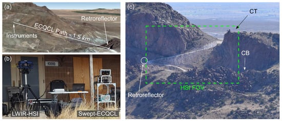
Figure 1.
Instrument locations at the plume release site. (a) Image from Google Earth showing locations of swept-ECQCL and hyperspectral imaging (LWIR-HSI) instruments, and retroreflector used with the swept-ECQCL instrument. (b) Photograph of LWIR-HSI and swept-ECQCL systems during measurements. (c) Photographic view looking SE from the vantage point of ECQCL and LWIR-HSI instruments. The cliff-top (CT) plume release location is visible, while the cliff-bottom (CB) location is not visible but lies behind a ridgeline in the foreground of the photograph. The dashed box shows the field of view (FOV) for the LWIR-HSI system, and the circle marks the location of the retroreflector.
Gas-phase plumes of SF6 and F152a were released from two locations with different local topographies. One release point was at a cliff-top location (CT), and a second release point was located near the corresponding cliff-bottom (CB) 55 m lower in elevation. The CT location was highly exposed to the prevailing winds, whereas the CB location was partly shielded from prevailing winds by the surrounding terrain. Figure 1c shows a photograph of the release region taken from the vantage point of the instruments. The CT plume release point is marked, while the CB location is not visible, lying behind a ridgeline in the foreground of the image. The approximate field of view for the LWIR-HSI is shown, and the position of the retroreflector is indicated.
Figure 2a shows an overhead image obtained from Google Earth of the region near the plume release points. Recent digital elevation data obtained from USGS were found to reproduce the local topography poorly, especially near the steep cliff face. The elevation errors were also noticeable in the Google Earth terrain maps. It was found that contour lines traced from a digitized historical 1979 topographic map reproduced the local topography with higher accuracy, as shown in Figure 2b. Figure 2c shows an elevation profile along the dashed grey line marked in Figure 2b. The topography data shows that the CB location was in a local depression defined by the cliffside and a nearby hill, indicated approximately by the shaded yellow regions in Figure 2, which could partially trap chemical plumes released in the vicinity depending on the prevailing wind direction. Figure 2 also shows that the ECQCL measurement path in the release area was located at an elevation between the CT and CB release points. The horizontal distances from the CT and CB release points to the measurement path were 85 and 130 m, respectively, measured perpendicular to the measurement path along a heading of 40° (NE). Three wind sensors (3-dimensional sonic anemometers) were located near the plume release sites and are indicated in Figure 2 by the labels WT (winds at the top of the cliff), WB (winds at the bottom of the cliff), and WR (winds near retroreflector position).
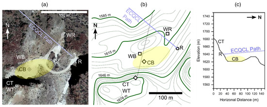
Figure 2.
Details of plume release site topography. (a) Overhead view obtained from Google Earth imagery. Labels indicate locations of retroreflector (R), plume release sites (CT, CB), and wind sensors (WT, WB, WR). (b) Topographic contour map showing elevation profile in release region (contour lines separated by 6 m). (c) Elevation profile along the path indicated by dashed grey line in (b). The elevations of the release locations (CT, CB) and retroreflector (R) are shown. The shaded yellow region in all panels indicates the presence of a local depressed area of elevation in which plumes could become partially trapped.
Two chemical tracers were used in the experiments. Sulfur hexafluoride (SF6) was released from a compressed gas cylinder at a regulated pressure of 10 psi and a constant rate of 4 g/s, with a duration of 10–15 min. 1,1-difluoroethane (F152a) was released from cans of commercial electronics dusters. Due to pressure variations as the cans were emptied, the release rate of F152a was less controlled than for SF6. An average release rate for F152a of 2.8 g/s was calculated based on the 840 g mass released over a duration of 5 min, with the release rate highest at the start of release and decaying to zero as the can approached empty.
2.2. Spatial-Temporal Plume Characterization Using Hyperspectral Imaging
The LWIR-HSI system (Telops Hyper-Cam LW) [29,34] is a commercial instrument with a spectral range of 7.7–11.8 μm (847–1298 cm−1), and a minimum resolution of 0.25 cm−1. The on-board HgCdTe camera has a format of 320 × 256 pixels and with the standard optic has a field of view of 6.4° × 5.1°, with each pixel having an individual field of view (iFOV) of 350 μrad (0.02°). The system also has an onboard high-definition visible color context camera. The Hyper-Cam LW has a radiometric accuracy of <1 K and a typical noise equivalent spectral radiance (NESR) of 20 nW/cm2-sr-cm−1. The sensor is housed in a weather-resistant enclosure and can operate from −20 °C–+40 °C. The instrument produces a calibrated output in radiance units, and this is achieved by the two on-board thermo-electric calibration blackbodies, which also provide uniformity correction for the HgCdTe camera. Data are output in ENVI format for viewing and post-processing. For this work, the region of interest (ROI) was reduced to 280 × 225 pixels and the spectral resolution was set to 6 cm−1 to scan and collect data as quickly as possible to map the dynamic plume movements. These settings resulted in an acquisition rate of one hypercube every 7 s. At a standoff distance of 1.5 km, each pixel mapped into a ground patch ~0.5 m on edge, giving a total scene dimension of 147 × 118 m.
The HSI data are analyzed by a ratio method to measure the relative signal absorbance using the following expression in Equation (1) applied to every pixel in the image ROI.
In Equation (1), the numerator Lsig(υ,t) is the observed signal radiance spectrum for times during the gas release, and Lbg(υ,t0) is the background radiance in the absence of the plume, obtained prior to each plume release. The absorption due to the SF6 plume was calculated by taking the difference in absorbance between spectral points on- and off-resonance with the strongest SF6 absorption peak:
For SF6 detection, = 946 cm−1 and = 955 cm−1 were used, based on the absorbance spectrum for SF6 shown below in Figure 3d. To form 2D plume maps, the processing methods in Equations (1) and (2) were applied to each pixel in the image for all data frames. The resultant differential absorbance values for each pixel were then grouped into 3 equal bins spanning the minimum to maximum absorbance values. The bins were assigned colors blue, green, and red (weak, medium, and strong absorption) and mapped onto the image showing the plume location and relative absorbance strength as a function of time and location for the release duration. The images were also arranged as an animation for a better understanding of plume dynamics as the SF6 is released and disperses in the complex terrain environment and under varying local wind conditions (examples are provided in the Supplementary Information). The SF6 absorbance measured by the LWIR-HSI system was also plotted at fixed locations as a function of time by averaging results in each image frame over multiple pixels. The approach used here to locate and plot the plume concentration is a simplified method compared to other plume quantification algorithms [27,28,29]; however, it provides an easily computed and semi-quantitative representation of the SF6 plume concentration that was found to be sufficient for the current analysis. A similar approach was used to measure the differential absorbance for the F152a plumes, but the lower absorption cross-section for F152a prevented reliable detection, and thus, the results are not presented here.
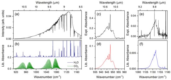
Figure 3.
Example spectra obtained with swept-ECQCL standoff system. (a) Measured intensity versus wavenumber/wavelength after propagation over an atmospheric path with 3 km total distance. The data are averaged over 10 s. (b) Library spectra for H2O and CO2 simulated using HITRAN parameters and scaled for a column density of 106 ppm × m. The spectra are offset for clarity. (c) Measured absorbance spectrum for SF6 (10 s average). (d) Library absorbance spectrum for SF6, scaled for 1 ppm × m. (e) Measured absorbance spectrum for F152a (10 s average). (f) Library absorbance spectrum for F152a scaled for 1 ppm × m.
2.3. High-Speed Plume Detection Using Standoff Swept-ECQCL System
The swept-ECQCL standoff detection hardware is a custom-built system that has been described previously in experiments at standoff ranges up to 900 m [18,38]. In the measurements here, the swept-ECQCL beam was directed to a retroreflector located at a standoff distance of 1.5 km by expanding the output beam to a 1/e2 diameter of ~50 mm using a negative lens with −15 mm focal length and off-axis parabola (OAP) with 230 mm focal length and 75 mm diameter. The expanded launch beam was aligned to the remote retroreflector using a 102 mm diameter flat mirror in a gimbal mount located after the OAP. Return light from the retroreflector was collected using a second 102 mm diameter flat mirror and 75 mm diameter OAP with 230 mm focal length. The return light was focused onto a thermoelectrically cooled infrared photodetector (VIGO PVI-4TE-10.6).
The swept-ECQCL system architecture and operation have been described in detail previously [9,18,38,40,41,42,43,44,45], and the reader is directed to these references for more information. Briefly, the swept-ECQCL used here included a QCL device (Thorlabs QE, Jessup, MD, USA) designed for broadband operation in the LWIR and which provided an overall tuning range of 910–1215 cm−1 (8.23–10.99 µm). For the measurements here, the tuning range was reduced to 915–1200 cm−1 (8.33–10.93 µm). The QCL was operated with amplitude-modulation (AM) of the current from 0–1500 mA using a 500 kHz square wave with a 50% duty cycle. The output of the ECQCL had a corresponding full-depth AM in intensity at 500 kHz, enabling lock-in detection of the ECQCL signal in the presence of ambient thermal infrared light on the photodetector. The signals from the infrared detectors were digitized at a 2 MHz rate using National Instruments hardware and demodulated in software written in LabVIEW, providing measurements of the detected ECQCL intensity at 2 µs intervals.
The swept-ECQCL wavenumber range was scanned at a 400 Hz rate (2.5 ms/scan). The average output power of the ECQCL in the launch beam at the peak of the tuning curve (1125 cm−1) was 6.5 mW, and the intensity was below the maximum permissible exposure (MPE) threshold of 100 mW/cm2 at all times for these infrared wavelengths.
Figure 3a shows an example of measured scan intensity from the swept-ECQCL system after propagation through the 3 km atmospheric path. The overall shape of the profile results from the gain bandwidth of the QCL device combined with wavelength-dependent reflectivity of optical elements inside and outside the ECQCL cavity and modified by the wavelength-dependent detector responsivity. The sharp spectral features show absorption by atmospheric H2O and CO2 along the 3000 m measurement path, and lines were resolved with spectral widths ~0.25–0.40 cm−1. Figure 3b shows absorption spectra for H2O and CO2 simulated using HITRAN parameters [46] for a column density of 106 ppm × m.
The measured intensity for each scan was converted to absorbance by , where is the average scan intensity for a background dataset. Thus, measures changes in the absorbance spectrum relative to the average conditions at the time the background was acquired. was taken from a 30 s average of scans obtained before each plume release was started. A longer background dataset was acquired over a 2-h time period during which no plume releases occurred for analysis of noise and drifts. A principal component analysis (PCA) was performed on the background dataset for use in fitting the absorbance spectral baseline [9,18,40], and 50 PC vectors were used for the baseline fitting.
Figure 3 shows examples of the measured absorption spectra averaged over 10 s, during which chemical plumes were detected along the measurement path. Figure 3c shows an example of a measured absorbance spectrum for SF6. Despite the low average power of the ECQCL in this region of the spectrum, the high cross-section for SF6 permits detection with a high signal-to-noise ratio (SNR). Figure 3d plots the library absorption spectrum for SF6 obtained from the PNNL spectral database [47], scaled for a column density of 1 ppm × m. Figure 3e shows an example measured spectrum for F152a, and Figure 3e shows the corresponding library absorption spectrum. In this case, the lower cross-section for F152a resulted in reduced signal levels but was partially compensated by the lower noise due to the higher ECQCL intensity. The large noise spikes result from spectral regions near strong H2O features, with corresponding low light levels reaching the detector. However, the broad absorption from F152a is easily recognized over the spectrally localized noise spikes.
Absorbance spectra at each measurement time were analyzed using a weighted least-squares (WLS) algorithm, which has been described previously [18]. The WLS algorithm provides the column density in units of ppm × m for each species as a function of time. To reduce the total computation time for the WLS analysis and to better match the time scales of the plume detections, the absorbance spectra were first averaged from the native 400 Hz acquisition rate to a 20 Hz rate. For plotting, the column densities were further averaged to a 1 Hz rate. The selection of a 1 Hz rate is based on the timescales of plume fluctuations observed during the experiments and is addressed in Appendix A.
3. Results
Plume Detection with Hyperspectral Imager and Standoff Swept-ECQCL Systems
Results from two plume-release experiments are presented, both conducted on 5 November 2019. In the first experiment, SF6 was released from the CB location at the bottom of the cliff, while F152a was released from the CT location at the top of the cliff. In the second experiment, the locations were switched with the SF6 released from the CT location and the F152a released from the CB location. In both experiments, the SF6 and F152a releases were initiated at the same time but with different durations.
Figure 4 shows wind data recorded onsite for the time periods corresponding to the two plume release experiments. Horizontal wind data are plotted as wind roses (direction from which winds were blowing), overlaid on an image from Google Earth at positions corresponding to the three wind sensors. The winds at the CT release point showed large turbulent variations over the release periods, but, on average, the winds were directed toward the N and W directions. The CT winds indicate that at some, but not all times, the winds had a component that would direct a plume toward the ECQCL path (see Figure 3a). The winds at the bottom of the cliff near the CB release point were directed toward the W and SW directions, flowing almost directly away from the ECQCL path. In contrast, the winds at the WR location were directed primarily to the NE Direction. Vertical wind speeds at the measured locations were on average 0 m/s over the release durations at all sensors, with a standard deviation of 0.4 m/s. However, the winds had localized periods of non-zero vertical wind components (upward+ or downward−) on ~1–10 s time scales. Overall, the varied wind fields in the release region are indicative of the complex terrain, which is expected to have a significant impact on the propagation of plumes released in the area.
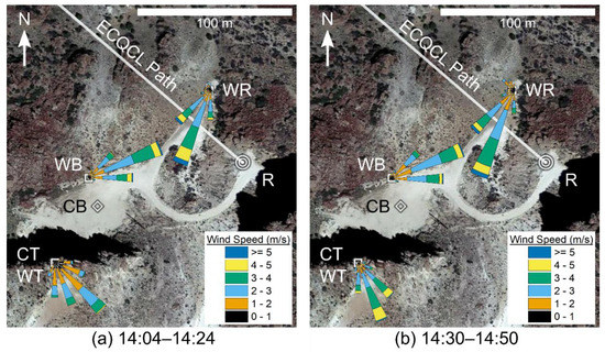
Figure 4.
Wind rose plots showing horizontal direction/speeds at ~2-m above ground level over time periods (local time hh:mm) (a) 14:04–14:24 and (b) 14:30–14:50, overlaid on an image from Google Earth. Labels are defined in Figure 2a.
Figure 5 shows results obtained using the LWIR-HSI system during a release of SF6 from the CB location. Figure 5a–f show images at the indicated local times, with the strength of SF6 absorption indicated by the color mapping: blue (weak), green (medium), and red (strong). An animation of the data, including additional times, is provided in the Supplementary Information. The detected plume is spatially inhomogeneous, with variations over length scales of meters (1 pixel ~0.5 m). Figure 5g shows the SF6 signal versus time, averaged over the spatial region marked by the solid yellow box in Figure 5a–f. The red bar shows the times during which SF6 was released. Figure 5g shows a delay of ~120 s between the start of the release and the first detection within the solid yellow box marked in Figure 5a–f, with a similar delay between the end of the release and the last detection, which is expected due to the spatial separation between the release location and the detection region. The plume initially moves toward the right in the images, away from the retroreflector location, which is consistent with the wind directions recorded near the CB release point shown in Figure 4a. The plume then appears to expand both laterally and vertically, the latter due to the expected downwind vortex that develops to the north of the cliff site for winds traveling roughly northwards. The vortex results in a downward motion at a finite distance to the north of the cliff face and upwards motion near the cliff face in the low-pressure zone, as well as lateral expansion of the SF6 tracer as it disperses into the “downwind” cavity zone. As the plume moves vertically toward the top of the cliff, portions of the plume are seen to move toward the left along the cliff face (roughly eastwards) in the direction of the canyon opening between the cliff-top peak and the hill to the ENE (see Figure 2b). At this point, some fraction of the canyon wind is expected to split off and channel towards the NE in a similar direction as measured at the WR sonic location and transport some of the tracers towards the retroreflector.
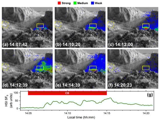
Figure 5.
Plume detection using an LWIR-HSI system during a release of SF6 from the CB location. (a–f) Images of detected SF6 at selected local times (hh:mm:ss). The dashed box shows the location of the retroreflector. Color mapping blue (weak), green (medium), and red (strong) shows the relative HSI absorption signal strength between zero and maximum, divided into three equal bins. (g) SF6 signal versus time averaged over the region in the solid yellow box. The solid red bar shows the times over which SF6 was released.
Figure 6a shows the SF6 signal versus time measured by the LWIR-HSI system, in this case averaged over the region near the retroreflector indicated by the dashed box in Figure 5 and corresponding to a region of 31 × 26 pixels. Figure 6b shows the SF6 column density measured by the swept-ECQCL standoff system. Despite the different measurement rates, the qualitative agreement between the SF6 detected by the LWIR-HSI and swept-ECQCL systems is excellent, providing important cross-validation of the results across the two different instruments. Figure 6c shows the F152a column density versus time detected using the swept-ECQCL system, which was below the detection limits for the LWIR-HSI system in this case.

Figure 6.
Time-resolved detection of plumes with SF6 released from the CB location and F152a released from the CT location. (a) SF6 signal versus time detected by LWIR-HSI in the spatial region near the retroreflector. (b) SF6 column density measured with the swept-ECQCL system. (c) F152a column density versus time measured with the swept-ECQCL system. The solid red and blue bars indicate the times over which SF6 and F152a were released, respectively.
The SF6 plume from the CB release location was first detected along the ECQCL measurement path after a delay of 300 s, giving an average propagation speed of 0.3 m/s. The SF6 plume was detected for times >500 s after the end of the release. Both these observations are consistent with the indirect propagation path for the SF6 plume from its release at CB to the retroreflector, as shown in Figure 5. In contrast, the F152a plume from the CT release location was first detected after a delay of 90 s, giving an average speed of 1.4 m/s. The F152a plume was detectable for <300 s after the release ended. This correlates with the idea that terrain can change the plume duration, with releases in a valley or canyon bottoms lasting longer due to being sheltered from the prevailing winds and mountain-top releases diluting more quickly due to being exposed to the full force of the prevailing wind.
Comparing the SF6 and F152a detection results from the swept-ECQCL system shows several interesting features. First, it is apparent that both SF6 and F152a are detected and distinguished, given the different time-dependences of the results. Both SF6 and F152a show fluctuations over fast (~second) time scales. However, the F152a was detected for ~200 s before the first detection of SF6, despite the larger distance from the F152a release at CT (130 m) versus SF6 at CB (85 m). This is likely due to a large fraction of the F152a tracer release at CT not getting caught in the slow-moving downwind vortex and instead taking a more direct path to the NE on average. There is a region between ~14:11 and 14:12 where SF6 and F152a were detected simultaneously with highly correlated time-dependence, suggesting that the plumes have mixed and are co-propagating at this time of detection. Finally, despite the near-continuous release rate of both tracers, the signals detected by the swept-ECQCL show large variations in column density, dropping to near zero at some times, indicative of the intermittent nature of the downwind cavity and turbulence in general.
Figure 7 shows results obtained using the LWIR-HSI system for the release of SF6 from the cliff-top CT location. Figure 7a–f show images at the indicated times, with the magnitude of SF6 absorption again indicated by the color mapping: blue (weak), green (medium), and red (strong). Figure 7g shows the SF6 absorbance signal versus time, averaged over the spatial region marked with the solid rectangle. The red bar shows the times over which SF6 was released. The release of SF6 from the CT location shows dramatically different behavior than when released from the CB location. Compared to the previous example, the plume is detected sooner after release and leaves the region near the release point more rapidly, partly due to imaging the plume closer to the release point. Figure 7b shows that the SF6 plume appears to split into two spatial components near the release point, with one component propagating toward the retroreflector location and the other traveling downward along the cliffside. The downward plume motion could be related to the high molecular weight of SF6 relative to the air, but local wind variability is also important. Smoke tracer experiments also performed at the site showed intermittent upward and downward motions of a visible plume near the cliff, indicative of the variability of the winds near the cliffside. Observations showed the downwind vortex sometimes directed the plume downwards, while at other times, the strong cliff-top wind instead lofted the plume horizontally away from the cliffside. Despite the continuous release of SF6, the plume detected near the release point shows large variations with time, as shown in Figure 7g, due to the variability of the prevailing wind speed and direction, turbulence intensity, and the downwind cavity zone. Comparison with the wind data in Figure 4a shows that the wind direction varied over the duration of the release, imparting temporal variations into the plume concentration at any given spatial location. Figure 7d,f also show that the plume was detected in the foreground direction of the image, indicating that part of the plume propagated over the ridgeline instead of being captured completely in the local depression at the bottom of the cliff site.
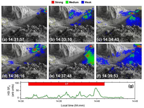
Figure 7.
Plume detection using LWIR-HSI system during a release of SF6 from the CT location. (a–f) Images of detected SF6 at selected times. The dashed box shows the location of the retroreflector. Color mapping blue (weak), green (medium), and red (strong) shows relative HSI signal strength between zero and maximum, divided into three equal bins. (g) SF6 signal versus time averaged over the region in the solid rectangle. The solid red bar shows the times over which SF6 was released.
Figure 8a shows the SF6 signal versus time from the LWIR-HSI data, averaged over the region near the retroreflector indicated by the dashed box in Figure 7. Figure 8b shows the SF6 column density measured by the swept-ECQCL standoff system. As with the previous example, the correlation in temporal signals between the SF6 detected by the LWIR-HSI and swept-ECQCL systems is excellent. Figure 8c shows the F152a column density versus time detected using the swept-ECQCL system, which, again, was below the detection limits for the LWIR-HSI system.
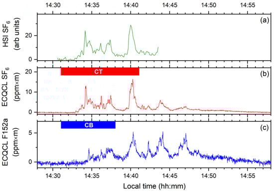
Figure 8.
Time-resolved detection of plumes for SF6 released from the CT location and F152a released from the CB location. (a) SF6 absorbance versus time detected by LWIR-HSI in the spatial region near the retroreflector. (b) SF6 column density measured with the swept-ECQCL system. (c) F152a column density versus time measured with the swept-ECQCL system. The solid red and blue bars indicate the times over which SF6 and F152a were released, respectively.
For this case of SF6 released from the CT location, the SF6 plume was detected by the ECQCL after a delay of ~120 s, giving an average plume speed of 1.1 m/s. The F152a plume from CB was detected after a longer delay of ~210 s, giving an average plume speed of 0.4 m/s. These average propagation times from CT and CB to the ECQCL path are similar to the previous experiment, but with the chemical species switched, indicating that, in these experiments, the topography influences the plume propagation more than the difference in chemical species. The plume detections of SF6 and F152a between 14:39 and 14:50 appear highly correlated, again suggesting that the plumes have mixed and are co-propagating at their time of detection at the ECQCL path. This observation is consistent with Figure 7, which shows a fraction of the SF6 traveling downwards north of the cliff, where it may mix with the F152a plume released from CB.
In addition to the plume detection experiments, additional measurements were performed onsite to characterize the swept-ECQCL and LWIR-HSI system performance. Appendix A provides an analysis of the swept-ECQCL measurements to determine timescales of atmospheric turbulence and timescales of plume concentration fluctuations. The results show that the 400 Hz wavelength scan rate of the swept-ECQCL was faster than the characteristic time scales of scintillation due to atmospheric turbulence at the measurement location. Frequency analysis of measured plume column densities is used to determine characteristic plume timescales of ~1 s, setting a maximum allowable averaging time for measurements to avoid a loss of accuracy in the retrieved chemical column densities [18].
4. Discussion
Combining the information from the wind sensors, LWIR-HSI system, and swept-ECQCL system provides a more complete picture of the plume propagation through complex terrain than any single measurement alone. The measured winds plotted in Figure 4 show large variations between points separated by <100 m and are influenced strongly by the local topography. For example, the exposed location at CT showed winds nearly perpendicular to those at a sheltered location at CB. As a result, plumes released from each of these locations followed very different propagation paths. Releases from the CT location were observed by the HSI system to take a more direct trajectory to the ECQCL measurement path, although SF6 was observed to split into multiple components influenced by the downwind vortex expected to exist near the cliff. Releases from the CB location were observed to become partially trapped by local topography, but the plumes experienced a different propagation behavior after they reached points higher up the cliffside and were exposed to winds in different directions. The more sensitive and higher-speed swept-ECQCL detection of tracers released simultaneously from different locations showed different dynamics initially after release, indicating different propagation paths from the release points. However, during later parts of the releases, the two tracers showed strong temporal correlations, suggesting a mixing of the two chemicals into a co-propagating plume.
Characterization of Performance for Swept-ECQCL and Hyperspectral Imaging Systems
In this section, we provide a detailed characterization of performance for the swept-ECQCL measurement system and comparisons with the commercial LWIR-HSI system. Figure 9 shows results from an Allan-Werle analysis [48] on a subset of data obtained using the swept-ECQCL over times during which no plumes were detected. Figure 9a,b show measured time-resolved column densities for SF6 and F152a over this period. In this case, the measurement results are expected to be zero apart from system noise and drifts; thus, the statistics of the actual measurement results provide a characterization of the noise/drifts in the measurement system. The Allan-Werle plot shown in Figure 9c provides a measure of noise-equivalent column density (NECD) for each species, which depends on the averaging time. For this analysis, a series of 80,000 scans obtained at the full 400 Hz scan rate (200 s total time) were analyzed to obtain the Allan deviation for times in the range 2.5–50 ms. A series of 144,000 scans were analyzed after averaging to a 20 Hz rate (2 h total time) to obtain the Allan deviation for times in the range of 50 ms–600 s.
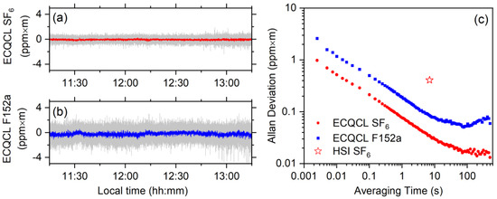
Figure 9.
Measured column density for (a) SF6 and (b) F152a during a 2-h background period with no plume releases. Light gray traces are for data analyzed at 20 Hz rate, and dark colored traces are data averaged to 1 Hz. (c) Allan deviation analysis of background data for column densities of SF6 (filled circles) and F152a (filled squares). The star indicates the noise-equivalent column density for SF6 detection using the LWIR-HSI system.
For the measurements reported here, the NECD improves with averaging of up to 10–100 s, with variations depending on species. For longer averaging times, slow drifts in the measured column densities lead to a small increase in NECD. The time scales of noise and drift relative to the time scales of plume variations are critical parameters for transient plume detection. For example, in the current situation, it is easy to distinguish the fast changes in column density occurring with ~1 s time scale as a plume intersects the beam path from instrumental drifts occurring with >100 s time scales.
Global average background levels of SF6 and F152a are ~10 ppt [49]. Considering the 3000 m total path of the swept-ECQCL measurement, these background levels correspond to a column density of 0.03 ppm × m. Given the large number of plume releases conducted throughout multiple days of testing, it is possible that local background levels were higher than global averages and/or showed slow variations over long time scales. If slow variations in the actual background levels occurred during the acquisition of the dataset used for the Allan deviation analysis, these changes would be indistinguishable from instrumental drifts. Thus, it may not be possible to distinguish the lower limit of the Allan deviation as resulting from instrumental drifts versus actual changes in background levels for these three chemicals.
Table 1 summarizes the results from the Allan-Werle analysis at various averaging times. The NECD for SF6 and F152a is 1.0 and 2.6 ppm × m, respectively, for a 2.5 ms averaging time. Although the plumes did not show fluctuations over these short time scales, the high measurement rate provides benefits for the detection of species in flames or chemicals associated with explosive events [38,40]. For the plume measurements here, the 1 s averaging time was used to match the timescales of the plume variations, which improves the NECD to 0.2–0.5 ppm × m for SF6 and F152a. While longer averaging times would improve the NECD further, as shown in Figure 9, it would also reduce the peak detected column densities of the species in the transient plumes, leading to limited or no improvement in actual SNR. At the same time, excessive averaging would reduce the accuracy of the measured instantaneous column densities, especially for the minima and maxima, as previously shown [18]. In the experiments here, the measured peak column densities for SF6 and F152a plumes were typically 5–10 ppm × m and were easily visible with high SNR at a 1-s averaging time.

Table 1.
Summary of Allan deviation analysis for the swept-ECQCL standoff detection system. The noise-equivalent column density (NECD) for each species is tabulated for various averaging times. Noise-equivalent concentrations (NEC) are calculated assuming each species fills the entire 3000 m measurement path.
The Allan-Werle analysis results can also be used to predict the noise-equivalent concentration (NEC) for species distributed over the entire 3000 m measurement path, such as for the detection of large plumes at long distances from the release point or for the detection of variations in ambient background levels of these chemicals. Table 1 lists these values as the full-path NEC in units of parts-per-trillion (ppt), for longer averaging times of 10 and 100 s. The results indicate that variations in these species at tens of ppt levels over 10–100-s time scales may be possible with the current measurement system. However, differentiating these variations from instrument drifts becomes more and more challenging as averaging times increase, and additional research is needed.
The measurement noise for the LWIR-HSI system was estimated from signal fluctuations in the absence of plume detections. From Figure 8a, between times 14:30:37 and 14:32:50, the standard deviation of the HSI SF6 signal was measured to be 0.84. To convert the arbitrary units of the HSI measurement to a quantitative SF6 column density, signal levels were compared with the simultaneous swept-ECQCL measurement, from which a calibration factor of 0.51 ppm × m/HSI units was obtained for SF6. Using this calibration factor, the estimated NECD for SF6 detection using the LWIR-HSI system was calculated to be 0.4 ppm × m, obtained with an integration time of 7 s and averaged over 806 pixels from the hyperspectral image. The NECD for SF6 using the LWIR-HSI system is plotted in Figure 9c and is ~10× higher than the corresponding NECD using the swept-ECQCL at a 7-s integration time.
Direct comparisons of NECD to other standoff detection instruments or techniques are challenging due to differences in detected species, large variations in the absorption cross-section with wavelength, and differences in methods of performance characterization. Comparisons of the swept-ECQCL NECD to various other standoff detection methods have previously shown that the swept-ECQCL typically achieves a better NECD for a given averaging time [18]. For example, standoff measurements using dual frequency comb spectroscopy at 3.03–3.64 µm for the detection of broadband-absorbing species acetone and isopropanol reported sensitivities of 2–6 ppm × m but required a long 60 s averaging time [50]. For standoff detection using other LWIR ECQCL systems, Goyal et al. reported a NECD for Freon-134a of 1 ppm × m at a 5 s averaging time and 155 m standoff distance [17]; F152a and SF6 were also detected, but NECD values were not provided. An active coherent laser spectrometer (ACLaS) system using a broadly tunable ECQCL scanned in 30 s was used to measure Freon-134a in a diffuse reflection standoff mode at 3 m, reporting a NECD of 10.5 ppm × m Hz−1/2 [15]. The results presented here for standoff detection using the swept-ECQCL at 1.5 km show NECD values of 0.08 and 0.19 ppm × m for SF6 and F152a at 1 s averaging. The NECD for F152a is slightly higher than our previous measurements using an LWIR swept-ECQCL at a 235-m standoff distance, which reported NECD values of 0.2 ppm × m at a 100 ms measurement time for Freon-134a and Freon-152a [18], with differences likely due to lower return signal intensity at a longer standoff range. The results show that the swept-ECQCL standoff detection system can obtain lower noise at higher speeds than other reported systems based on broadband-active infrared absorption spectroscopy.
In terms of SF6 detection, the results obtained with the swept-ECQCL and LWIR-HSI instruments can be compared directly with other standoff detection methods. SF6 has been detected in active standoff measurements using differential absorption lidar (DIAL) based on line-tunable CO2 lasers [23]. The detection of an SF6 plume at a range of 16 km was demonstrated using DIAL with light reflected from a topographic target [51]. An airborne DIAL system was used to measure SF6 with estimated detection limits of 2 ppm × m at a 2 Hz measurement rate [24]. DIAL has the advantages of operating at long range and providing range-resolved measurements in some configurations; however, the use of two wavelengths provides little or no resistance to spectral interferences from gas species other than the one targeted. The swept-ECQCL standoff system provides lower detection limits for SF6 than these DIAL systems, with the added benefit of full spectral acquisition for multi-species and mixture detection.
For passive standoff methods, SF6 was detected using differential FTIR radiometry at a standoff distance of 5.7 km with an estimated precision of 16 ppm × m at a 1 s measurement time [52]. SF6 was detected using passive FTIR at 200 m, with a calculated noise-equivalent concentration length of 0.5 ppm × m [28]. The Telops Hypercam LWIR-HSI instrument is commercially available; however, significant variation in performance may occur based on the measurement configuration and environment (thermal contrast, range, magnification, field-of-view, spectral resolution, etc.). The gas measured and spectral analysis procedure will also influence the results. Previous measurements of SF6 plumes using Telops instrumentation have been reported [29,35,36,37], and in Hirsch and Agassi [37], a detection limit for SF6 was reported as 30.5 mg/m2 (5 ppm × m) with a 4 s measurement time. The results obtained here using the Telops LWIR-HSI system showed a NECD of 0.4 ppm × m, obtained with an integration time of 7 s, which is similar to values previously reported considering measurement differences.
The accuracy of the column densities measured by the instruments is difficult to assess because it is usually not practical to calibrate a standoff detection system operating in open-air to a known and stable quantity of a reference gas [35]. Previous measurements have demonstrated the ability of swept-ECQCL instrumentation to record absorbance spectra with high accuracy when compared with library reference spectra [9,18,38,41,42,43,44,45,53]. Assuming an accurate measurement of the absorbance spectrum, the primary sources of uncertainty in column density are the absorbance cross-section data accuracy and the ability to perform an accurate spectral fit. One source of uncertainty in the accuracy of the retrieved column density could occur due to temperature variations along the measurement path. Based on the temperature dependence from 5–50 °C of the infrared absorption cross-sections for the SF6 and F152a bands measured here [47], we estimate uncertainty in the retrieval of column densities of no more than 10% for a 5 °C variation in temperature along the measurement path. This uncertainty is comparable to the typical uncertainty in the magnitudes of the cross-sections [47].
The swept-ECQCL measurements detected peak column densities of ~5–15 ppm × m for the plume experiments reported here. To estimate the expected plume column density for the SF6 release, a simple Gaussian plume model [54] was performed using the location and weather conditions on the day of the tests, with an SF6 release rate of 4 g/s and a constant wind speed of 1 m/s. Under these conditions, the predicted column density is ~25 ppm × m at a distance of ~130 m downwind of the release point (with a predicted plume width of ~130 m). The Gaussian plume model gives a rough order-of-magnitude prediction for the column density and indicates that the magnitudes of column densities measured by the swept-ECQCL are reasonable given the plume release parameters. However, the Gaussian plume model does not account for local topography and local wind variations, both of which are important for short-range plume propagation. Furthermore, the Gaussian plume model does not account for the observed rapid time-dependence in the plume column density.
Additional confidence in the accuracy of the results is provided by the good agreement between the swept-ECQCL and LWIR-HSI measurements shown in Figure 6 and Figure 8. Although the LWIR-HSI results were not calibrated independently in terms of column density, the agreement in relative magnitudes and time-dependence with the swept-ECQCL results provides partial cross-validation between the two independent measurements. Overall, the statistical evaluation of NECD using the Allen-Werle deviation, combined with the agreement between the swept-ECQCL and LWIR-HSI measurements, provides high confidence in the sensitivity and relative accuracy of retrieved column densities. Absolute accuracy of column densities will be linked to the accuracy of absorption cross-section data and spectral fitting performance, but the measured values are reasonable when compared with Gaussian plume dispersion models.
5. Conclusions
In this manuscript, we have presented results from outdoor plume release measurements in complex terrain, with plume detection using two complementary measurement techniques. One measurement used a passive LWIR-HSI system to provide a time-series of hyperspectral images used to locate SF6 plumes spatially and track their propagation through the scene. The second measurement used an active-mode swept-ECQCL system to measure plume column densities at high speed and high sensitivity along a line located away from the plume release locations. Both systems were operated in a standoff configuration and were located at a 1.5 km distance from the plume release locations. Two plume propagation configurations were studied, with gas-phase tracers released simultaneously from an exposed cliff-top and from a sheltered cliff-bottom.
The plume release experiments show the complicated nature of short-range plume transport through complex terrain. Measured winds showed large variations between points separated by <100 m and were strongly influenced by the local topography. Tracers released simultaneously from the different locations showed different initial dynamics but were found to mix and form a co-propagating plume at later times. The results confirm that the site topography and local winds near a plume release point strongly affect the plume propagation for short distances and times. As a result, plumes released from different locations may be distinguishable based on their temporal dynamics. For later times in plume transport and at longer distances, plumes from different release points may mix, or they may be distinct based on the specifics of the microscale winds and turbulent mixing.
In terms of instrument performance in the current experiments, the LWIR-HSI system provided passive detection from a standoff distance of 1.5 km and imaged a large spatial area, with large spectral bandwidth in the LWIR (450 cm−1), moderate spectral resolution (6 cm−1), and moderate temporal resolution (7 s). The 7 s temporal response of the system was not sufficient to capture the rapid ~1 s fluctuations in plume dynamics revealed using the swept-ECQCL measurements. The passive-mode detection of the LWIR-HSI system allowed measurement without the need for an emplaced retroreflector; however, detection of passive infrared radiation makes quantitative plume measurements more challenging and limits the sensitivity. The time-resolved hyperspectral images are extremely valuable for locating the chemical plume release and characterizing its spatial and temporal evolution through the scene. The SF6 plumes were detected with high SNR near the release point due to the high concentrations, with SNR decreasing at larger distances due to dilution of the plume. Nevertheless, with a relatively simple spectral analysis approach to isolate the SF6 absorption from the background and averaging over multiple pixels in the image, the SF6 plume was detected at distances ~100 m away from the release points above the calculated noise level of 0.4 ppm × m. In general, results may vary depending on operating parameters for the instrument (spectral resolution, frame rate, image magnification, etc.), scene properties (background radiance and contrast with the plume), chemical species detected (absorption cross-section within detection spectral bandwidth), and spectral processing/analysis approach.
The swept-ECQCL system also operated in the LWIR at a standoff distance of 1.5 km, with a spectral bandwidth of 250 cm−1, a spectral resolution of ~0.3 cm−1, and a scan time of 2.5 ms, but only measured along a single line-of-sight within the scene. The high scan speed was used to reduce noise from atmospheric turbulence and enabled the measurement to track the fluctuations in the plume column density occurring over a ~1 s time scale. The swept-ECQCL measurement enabled high-SNR and high-speed measurements of plume column density at a location ~100 m away from the plume release points and detected not only the SF6 plumes but also the weaker F152a plumes with lower absorption cross-section and lower average column density. For an integration time of 1 s, the NECD was measured to be 0.08 ppm × m for SF6 and 0.19 ppm × m for F152a. As with the HSI system, measurement performance is expected to vary with instrument operating parameters (scan bandwidth, scan speed, integration time), measurement geometry (standoff distance, distance of measurement path from the plume), scene properties (atmospheric conditions), and chemical species.
Combining the measurement results from the LWIR-HSI and the swept-ECQCL provides a more complete picture of the plume propagation than either method alone. Since the spatial and temporal properties of plume propagation are linked, simultaneous measurement of both is important for the characterization of plume evolution. Furthermore, the quantitative swept-ECQCL measurements can be used to provide in-scene calibrations for the HSI plume measurements that do not depend on radiance or thermal contrast, greatly simplifying the determination of plume column density. Both instruments are operated in an optical standoff configuration and thus require a visible line-of-sight to the points at which the plume is detected; however, neither require the actual plume release point to be imaged or detected. Similarly, because no physical contact with the plume is required, these standoff methods provide important capabilities useful for plume propagation measurement and quantification in complex or mountainous terrain with limited access.
Supplementary Materials
The following supporting information can be downloaded at: https://www.mdpi.com/article/10.3390/rs14153756/s1, Figure S1. Animation showing a cliff bottom release of SF6 beginning at time 14:04:03 and ending at 14:20:49 resulting in 158 hypercubes with one hypercube recorded every ~7 s. This is the release described in the text in Figure 6, which the color scale corresponds to strong signal detection (red), medium strength detection (green) and weak detection (blue). Figure S2. Animation showing a cliff top release of SF6 beginning at time 14:30:37 and ending at 14:32:31, resulting in 118 hypercubes. This is the release described in Figure 8 of the text. Animation S1: HSI Results for 1405 Plume. Animation S2: HSI Results for 1431 Plume.
Author Contributions
Conceptualization, all authors; investigation, all authors; data analysis, M.C.P. and B.E.B.; writing—original draft preparation, M.C.P. and B.E.B.; writing—review and editing, all authors. All authors have read and agreed to the published version of the manuscript.
Funding
This work was partly supported by the National Nuclear Security Administration, Defense Nuclear Nonproliferation R&D Office, and the Department of Energy Phase I SBIR program (No. DE-SC0019855). The Pacific Northwest National Laboratory is operated for the U.S. Department of Energy (DOE) by the Battelle Memorial Institute under Contract No. DE-AC05-76RL01830.
Data Availability Statement
The data presented in this study are available on request from the corresponding author.
Acknowledgments
We thank Jeremy Yeak for assistance with the swept-ECQCL experimental measurements and also thank the staff from EMRTC for onsite support during the measurement campaign. The authors acknowledge important interdisciplinary collaboration with scientists and engineers from multiple DOE National Laboratories, including LANL, LLNL, MSTS, PNNL, and SNL.
Conflicts of Interest
One author (Mark C. Phillips) is an employee of a small business (Opticslah. LLC).
Appendix A. High-Speed Plume Characterization Using Swept-ECQCL Instrument
This section contains an additional characterization of the swept-ECQCL measurement system pertaining to its use for high-speed plume detection. To characterize the effects of atmospheric turbulence over the 3000 m propagation path, the swept-ECQCL was operated in a non-scanning mode at a fixed wavenumber of 1040 cm−1, and the detected signal was digitized at a 500 kHz rate. Figure A1a shows a representative section of data obtained over a 1s time period. The effects of atmospheric turbulence are apparent via the fluctuations in the detected laser power. For the data shown in Figure A1a, the calculated scintillation index was = 0.15, where gives the normalized variance of the detected intensity fluctuations [55]. Figure A1b plots a temporal autocorrelation of the signal in Figure A1a and shows that the return signals become uncorrelated over millisecond time scales, with a 3 dB point at 5.8 ms. The results confirm that the 2.5 ms time required to obtain each wavelength scan using the swept-ECQCL is shorter than characteristic time scales of atmospheric turbulence.
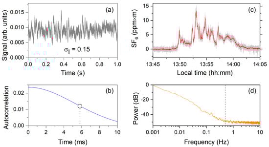
Figure A1.
Temporal characterization of atmosphere and plume dynamics using swept-ECQCL. (a) Temporal variations in return power at a fixed wavelength over a 1 s time period due to scintillation. The detector signal was digitized at a 500 kHz rate for these measurements, and the calculated scintillation index over this time period was = 0.15. (b) Temporal autocorrelation of signal in (a). The dashed line shows the 3 dB point at 5.8 ms. (c) Measured time-resolved column density for SF6 in the plume release experiment. The light gray trace shows results after averaging to 20 Hz, and the dark red trace shows results after averaging to 1 Hz. (d) Fourier transform (power spectrum) of 20 Hz results shown in (c). The dashed line shows the frequency (~0.5 Hz) above which the plume has negligible signal power.

Figure A1c shows an example of the time-resolved SF6 column density detected using the swept-ECQCL instrument after spectral analysis. The light gray trace shows results from analysis of spectra averaged to 20 Hz (50 ms). The dark red trace shows the column density after averaging the 20 Hz column density to a 1 Hz rate (1 s). Figure A1d shows a power spectrum obtained from a Fourier transform of the 20 Hz SF6 column density shown in Figure A1c. The power spectrum in Figure A1d shows that the temporal fluctuations in plume column density at the location probed by the swept-ECQCL occur at frequencies 0.5 Hz. Therefore, 1 s was selected as an optimum averaging time to capture the full frequency content of the plumes (sampling at 2× the maximum frequency) while allowing reduction of noise via averaging.
References
- Steyn, D.; De Wekker, S.; Kossmann, M.; Martilli, A. Boundary Layers and Air Quality in Mountainous Terrain. In Mountain Weather Research and Forecasting; Chow, F., De Wekker, S., Snyder, B., Eds.; Springer: Dordrecht, The Netherlands, 2013; pp. 261–289. ISBN 978-94-007-4097-6. [Google Scholar]
- Giovannini, L.; Ferrero, E.; Karl, T.; Rotach, M.W.; Staquet, C.; Trini Castelli, S.; Zardi, D. Atmospheric Pollutant Dispersion over Complex Terrain: Challenges and Needs for Improving Air Quality Measurements and Modeling. Atmosphere 2020, 11, 646. [Google Scholar] [CrossRef]
- Fernando, H.J.S.; Pardyjak, E.R.; Di Sabatino, S.; Chow, F.K.; De Wekker, S.F.J.; Hoch, S.W.; Hacker, J.; Pace, J.C.; Pratt, T.; Pu, Z.; et al. The Materhorn: Unraveling the Intricacies of Mountain Weather. Bull. Am. Meteorol. Soc. 2015, 96, 1945–1967. [Google Scholar] [CrossRef]
- Whiteman, C.D. Mountain Meteorology: Fundamentals and Applications; Oxford University Press: New York, NY, USA, 2000; ISBN 978-0-19-513271-7. [Google Scholar]
- Zardi, D.; Rotach, M.W. Transport and Exchange Processes in the Atmosphere over Mountainous Terrain: Perspectives and Challenges for Observational and Modelling Systems, from Local to Climate Scales. Atmosphere 2021, 12, 199. [Google Scholar] [CrossRef]
- Sekiyama, T.T.; Kajino, M. Reproducibility of Surface Wind and Tracer Transport Simulations over Complex Terrain Using 5-, 3-, and 1-Km-Grid Models. J. Appl. Meteorol. Climatol. 2020, 59, 937–952. [Google Scholar] [CrossRef] [Green Version]
- Costigan, K.R. Tracking Virtual, Atmospheric Emissions from Time-Varying and Short-Term Sources During the DNE18 Study Time Period. In Proceedings of the AGU Fall Meeting, Washington, DC, USA, 1 December 2018. [Google Scholar]
- Wagenbrenner, N.S.; Forthofer, J.M.; Lamb, B.K.; Shannon, K.S.; Butler, B.W. Downscaling Surface Wind Predictions from Numerical Weather Prediction Models in Complex Terrain with Windninja. Atmos. Chem. Phys. 2016, 16, 5229–5241. [Google Scholar] [CrossRef] [Green Version]
- Phillips, M.C.; Taubman, M.S.; Bernacki, B.E.; Cannon, B.D.; Stahl, R.D.; Schiffern, J.T.; Myers, T.L. Real-Time Trace Gas Sensing of Fluorocarbons Using a Swept-Wavelength External Cavity Quantum Cascade Laser. Analyst 2014, 139, 2047–2056. [Google Scholar] [CrossRef]
- You, Y.; Staebler, R.M.; Moussa, S.G.; Su, Y.; Munoz, T.; Stroud, C.; Zhang, J.; Moran, M.D. Long-Path Measurements of Pollutants and Micrometeorology over Highway 401 in Toronto. Atmos. Chem. Phys. 2017, 17, 14119–14143. [Google Scholar] [CrossRef] [Green Version]
- Griffith, D.W.T.; Pohler, D.; Schmitt, S.; Hammer, S.; Vardag, S.N.; Platt, U. Long Open-Path Measurements of Greenhouse Gases in Air Using near-Infrared Fourier Transform Spectroscopy. Atmos. Meas. Tech. 2018, 11, 1549–1563. [Google Scholar] [CrossRef] [Green Version]
- Akagi, S.K.; Burling, I.R.; Mendoza, A.; Johnson, T.J.; Cameron, M.; Griffith, D.W.T.; Paton-Walsh, C.; Weise, D.R.; Reardon, J.; Yokelson, R.J. Field Measurements of Trace Gases Emitted by Prescribed Fires in Southeastern US Pine Forests Using an Open-Path FTIR System. Atmos. Chem. Phys. 2014, 14, 199–215. [Google Scholar] [CrossRef] [Green Version]
- Yokelson, R.J.; Griffith, D.W.T.; Ward, D.E. Open-Path Fourier Transform Infrared Studies of Large-Scale Laboratory Biomass Fires. J. Geophys. Res. Atmos. 1996, 101, 21067–21080. [Google Scholar] [CrossRef] [Green Version]
- Li, J.; Yu, Z.; Du, Z.; Ji, Y.; Liu, C. Standoff Chemical Detection Using Laser Absorption Spectroscopy: A Review. Remote Sens. 2020, 12, 2771. [Google Scholar] [CrossRef]
- Macleod, N.A.; Molero, F.; Weidmann, D. Broadband Standoff Detection of Large Molecules by Mid-Infrared Active Coherent Laser Spectrometry. Opt. Express 2015, 23, 912–928. [Google Scholar] [CrossRef]
- Macleod, N.A.; Rose, R.; Weidmann, D. Middle Infrared Active Coherent Laser Spectrometer for Standoff Detection of Chemicals. Opt. Lett. 2013, 38, 3708–3711. [Google Scholar] [CrossRef] [PubMed]
- Goyal, A.K.; Kotidis, P.; Deutsch, E.R.; Zhu, N.; Norman, M.; Ye, J.; Zafiriou, K.; Mazurenko, A. Detection of Chemical Clouds Using Widely Tunable Quantum Cascade Lasers. Proc. SPIE 2015, 9455, 94550L. [Google Scholar] [CrossRef]
- Phillips, M.C.; Bernacki, B.E.; Harilal, S.S.; Yeak, J.; Jones, R.J. Standoff Chemical Plume Detection in Turbulent Atmospheric Conditions with a Swept-Wavelength External Cavity Quantum Cascade Laser. Opt. Express 2020, 28, 7408–7424. [Google Scholar] [CrossRef] [PubMed]
- Rieker, G.B.; Giorgetta, F.R.; Swann, W.C.; Kofler, J.; Zolot, A.M.; Sinclair, L.C.; Baumann, E.; Cromer, C.; Petron, G.; Sweeney, C.; et al. Frequency-Comb-Based Remote Sensing of Greenhouse Gases over Kilometer Air Paths. Optica 2014, 1, 290–298. [Google Scholar] [CrossRef] [Green Version]
- Nikodem, M.; Wysocki, G. Chirped Laser Dispersion Spectroscopy for Remote Open-Path Trace-Gas Sensing. Sensors 2012, 12, 16466–16481. [Google Scholar] [CrossRef]
- Kara, O.; Sweeney, F.; Rutkauskas, M.; Farrell, C.; Leburn, C.G.; Reid, D.T. Open-Path Multi-Species Remote Sensing with a Broadband Optical Parametric Oscillator. Opt. Express 2019, 27, 21358–21366. [Google Scholar] [CrossRef] [PubMed]
- Winker, D.M.; Hunt, W.H.; McGill, M.J. Initial Performance Assessment of Caliop. Geophys. Res. Lett. 2007, 34. [Google Scholar] [CrossRef] [Green Version]
- Kariminezhad, H.; Parvin, P.; Borna, F.; Bavali, A. SF6 Leak Detection of High-Voltage Installations Using TEA-CO2 Laser-Based DIAL. Opt. Lasers Eng. 2010, 48, 491–499. [Google Scholar] [CrossRef]
- Uthe, E.E. Airborne CO2 Dial Measurement of Atmospheric Tracer Gas Concentration Distributions. Appl. Opt. 1986, 25, 2492–2498. [Google Scholar] [CrossRef] [PubMed]
- Pappalardo, G.; Amodeo, A.; Apituley, A.; Comeron, A.; Freudenthaler, V.; Linné, H.; Ansmann, A.; Bösenberg, J.; D’Amico, G.; Mattis, I.; et al. Earlinet: Towards an Advanced Sustainable European Aerosol Lidar Network. Atmos. Meas. Tech. 2014, 7, 2389–2409. [Google Scholar] [CrossRef] [Green Version]
- Ghandehari, M.; Aghamohamadnia, M.; Dobler, G.; Karpf, A.; Buckland, K.; Qian, J.; Koonin, S. Mapping Refrigerant Gases in the New York City Skyline. Sci. Rep. 2017, 7, 2375. [Google Scholar] [CrossRef] [PubMed] [Green Version]
- Polak, M.L.; Hall, J.L.; Herr, K.C. Passive Fourier-Transform Infrared Spectroscopy of Chemical Plumes: An Algorithm for Quantitative Interpretation and Real-Time Background Removal. Appl. Opt. 1995, 34, 5406–5412. [Google Scholar] [CrossRef] [PubMed]
- Hu, Y.; Xu, L.; Shen, X.; Jin, L.; Xu, H.; Deng, Y.; Liu, J.; Liu, W. Reconstruction of a Leaking Gas Cloud from a Passive FTIR Scanning Remote-Sensing Imaging System. Appl. Opt. 2021, 60, 9396–9403. [Google Scholar] [CrossRef]
- Saute, B.; Gagnon, J.-P.; Duval, M.; Thibodeau, J.; Gagnon, M.; Lariviere-Bastien, M. Detection, Identification, and Quantification of SF6 Point-Source Emissions Using Telops Hyper-Cam Lw Airborne Platform. Proc. SPIE 2021, 11727, 273–279. [Google Scholar] [CrossRef]
- Bernacki, B.E.; Phillips, M.C. Standoff Hyperspectral Imaging of Explosives Residues Using Broadly Tunable External Cavity Quantum Cascade Laser Illumination. Proc. SPIE 2010, 7665, 7665. [Google Scholar] [CrossRef]
- Phillips, M.C.; Ho, N. Infrared Hyperspectral Imaging Using a Broadly Tunable External Cavity Quantum Cascade Laser and Microbolometer Focal Plane Array. Opt. Express 2008, 16, 1836–1845. [Google Scholar] [CrossRef]
- Goyal, A.; Myers, T.; Wang, C.A.; Kelly, M.; Tyrrell, B.; Gokden, B.; Sanchez, A.; Turner, G.; Capasso, F. Active Hyperspectral Imaging Using a Quantum Cascade Laser (QCL) Array and Digital-Pixel Focal Plane Array (DFPA) Camera. Opt. Express 2014, 22, 14392–14401. [Google Scholar] [CrossRef]
- Fuchs, F.; Hugger, S.; Kinzer, M.; Aidam, R.; Bronner, W.; Lösch, R.; Yang, Q.; Degreif, K.; Schnrer, F. Imaging Standoff Detection of Explosives Using Widely Tunable Midinfrared Quantum Cascade Lasers. Opt. Eng. 2010, 49, 111127. [Google Scholar] [CrossRef]
- Chamberland, M.; Farley, V.; Vallières, A.; Villemaire, A.; Belhumeur, L.; Giroux, J.; Legault, J.-F. High-Performance Field-Portable Imaging Radiometric Spectrometer Technology for Hyperspectral Imaging Applications. Proc. SPIE 2005, 5994, 59940N. [Google Scholar] [CrossRef]
- Hirsch, E.; Agassi, E.; Manor, A. Using Longwave Infrared Hyperspectral Imaging for a Quantitative Atmospheric Tracer Monitoring in Outdoor Environments. Int. J. Geosci. 2021, 12, 233–252. [Google Scholar] [CrossRef]
- Agassi, E.; Hirsch, E.; Chamberland, M.; Gagnon, M.A.; Eichstaedt, H. Detection of Gaseous Plumes in Airborne Hyperspectral Imagery. Proc. SPIE 2016, 9824, 9824. [Google Scholar] [CrossRef]
- Hirsch, E.; Agassi, E. Detection of Gaseous Plumes in IR Hyperspectral Images-Performance Analysis. IEEE Sens. J. 2010, 10, 732–736. [Google Scholar] [CrossRef]
- Phillips, M.C.; Harilal, S.S.; Yeak, J.; Jones, R.J.; Wharton, S.; Bernacki, B.E. Standoff Detection of Chemical Plumes from High Explosive Open Detonations Using Swept-Wavelength External Cavity Quantum Cascade Lasers. J. Appl. Phys. 2020, 128, 163103. [Google Scholar] [CrossRef]
- Brown, M.J.; Conry, P.; Nelson, M.; Boukhalfa, H.; Brug, P.; Rahn, T. An Overview of the EMRTC Complex-Terrain Dual-Tracer Experiment. LANL Report LA-UR-20-27800. 2020.
- Phillips, M.C.; Myers, T.L.; Johnson, T.J.; Weise, D.R. In-Situ Measurement of Pyrolysis and Combustion Gases from Biomass Burning Using Swept Wavelength External Cavity Quantum Cascade Lasers. Opt. Express 2020, 28, 8680. [Google Scholar] [CrossRef]
- Phillips, M.C.; Brumfield, B.E. Standoff Detection of Turbulent Chemical Mixture Plumes Using a Swept External Cavity Quantum Cascade Laser. Opt. Eng. 2018, 57, 011003. [Google Scholar] [CrossRef]
- Phillips, M.C.; Brumfield, B.E.; Harilal, S.S. Real-Time Standoff Detection of Nitrogen Isotopes in Ammonia Plumes Using a Swept External Cavity Quantum Cascade Laser. Opt. Lett. 2018, 43, 4065–4068. [Google Scholar] [CrossRef]
- Brumfield, B.E.; Phillips, M.C. Quantitative Isotopic Measurements of Gas-Phase Alcohol Mixtures Using a Broadly Tunable Swept External Cavity Quantum Cascade Laser. Analyst 2017, 142, 2354–2362. [Google Scholar] [CrossRef]
- Brumfield, B.E.; Taubman, M.S.; Phillips, M.C. Rapid and Sensitive Quantification of Isotopic Mixtures Using a Rapidly-Swept External Cavity Quantum Cascade Laser. Photonics 2016, 3, 33. [Google Scholar] [CrossRef] [Green Version]
- Brumfield, B.E.; Taubman, M.S.; Suter, J.D.; Phillips, M.C. Characterization of a Swept External Cavity Quantum Cascade Laser for Rapid Broadband Spectroscopy and Sensing. Opt. Express 2015, 23, 25553–25569. [Google Scholar] [CrossRef] [PubMed]
- Gordon, I.E.; Rothman, L.S.; Hill, C.; Kochanov, R.V.; Tan, Y.; Bernath, P.F.; Birk, M.; Boudon, V.; Campargue, A.; Chance, K.V.; et al. The HITRAN2016 Molecular Spectroscopic Database. J. Quant. Spectrosc. Radiat. Transf. 2017, 203, 3–69. [Google Scholar] [CrossRef]
- Sharpe, S.W.; Johnson, T.J.; Sams, R.L.; Chu, P.M.; Rhoderick, G.C.; Johnson, P.A. Gas-Phase Databases for Quantitative Infrared Spectroscopy. Appl. Spectrosc. 2004, 58, 1452–1461. [Google Scholar] [CrossRef] [PubMed]
- Werle, P.; Mucke, R.; Slemr, F. The Limits of Signal Averaging in Atmospheric Trace-Gas Monitoring by Tunable Diode-Laser Absorption-Spectroscopy (TDLAS). Appl. Phys. B 1993, 57, 131–139. [Google Scholar] [CrossRef]
- NOAA Global Monitoring Laboratory: Long-Term Global Trends of Atmospheric Trace Gases. Available online: https://gml.noaa.gov/hats/data.html (accessed on 1 March 2022).
- Ycas, G.; Giorgetta, F.R.; Cossel, K.C.; Waxman, E.M.; Baumann, E.; Newbury, N.R.; Coddington, I. Mid-Infrared Dual-Comb Spectroscopy of Volatile Organic Compounds across Long Open-Air Paths. Optica 2019, 6, 165–168. [Google Scholar] [CrossRef]
- Carlisle, C.B.; van der Laan, J.E.; Carr, L.W.; Adam, P.; Chiaroni, J.P. CO2 Laser-Based Differential Absorption Lidar System for Range-Resolved and Long-Range Detection of Chemical Vapor Plumes. Appl. Opt. 1995, 34, 6187–6200. [Google Scholar] [CrossRef]
- Lavoie, H.; Puckrin, E.; Thériault, J.M.; Bouffard, F. Passive Standoff Detection of SF6 at a Distance of 5.7 Km by Differential Fourier Transform Infrared Radiometry. Appl. Spectrosc. 2005, 59, 1189–1193. [Google Scholar] [CrossRef]
- Phillips, M.; Bernacki, B.; Harilal, S.; Brumfield, B.; Schwallier, J.; Glumac, N. Characterization of High-Explosive Detonations Using Broadband Infrared External Cavity Quantum Cascade Laser Absorption Spectroscopy. J. Appl. Phys. 2019, 126, 093102. [Google Scholar] [CrossRef] [Green Version]
- Gaussian Plume Model (Noaa.Gov). Available online: https://www.ready.noaa.gov/READY_gaussian.php (accessed on 1 March 2022).
- Andrews, L.C.; Phillips, R.L.; Hopen, C.Y. Laser Beam Scintillation with Applications; SPIE Press: Bellingham, WA, USA, 2001; ISBN 978-0-81-944103-4. [Google Scholar]

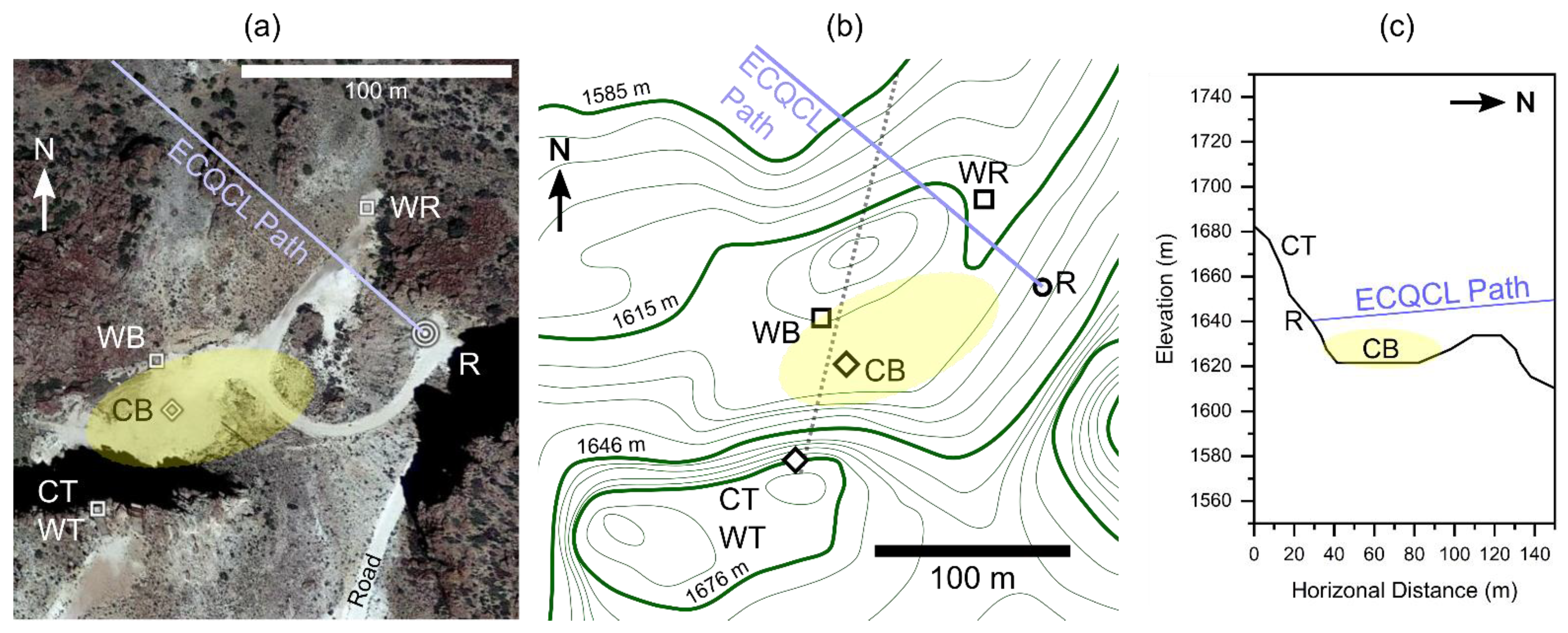
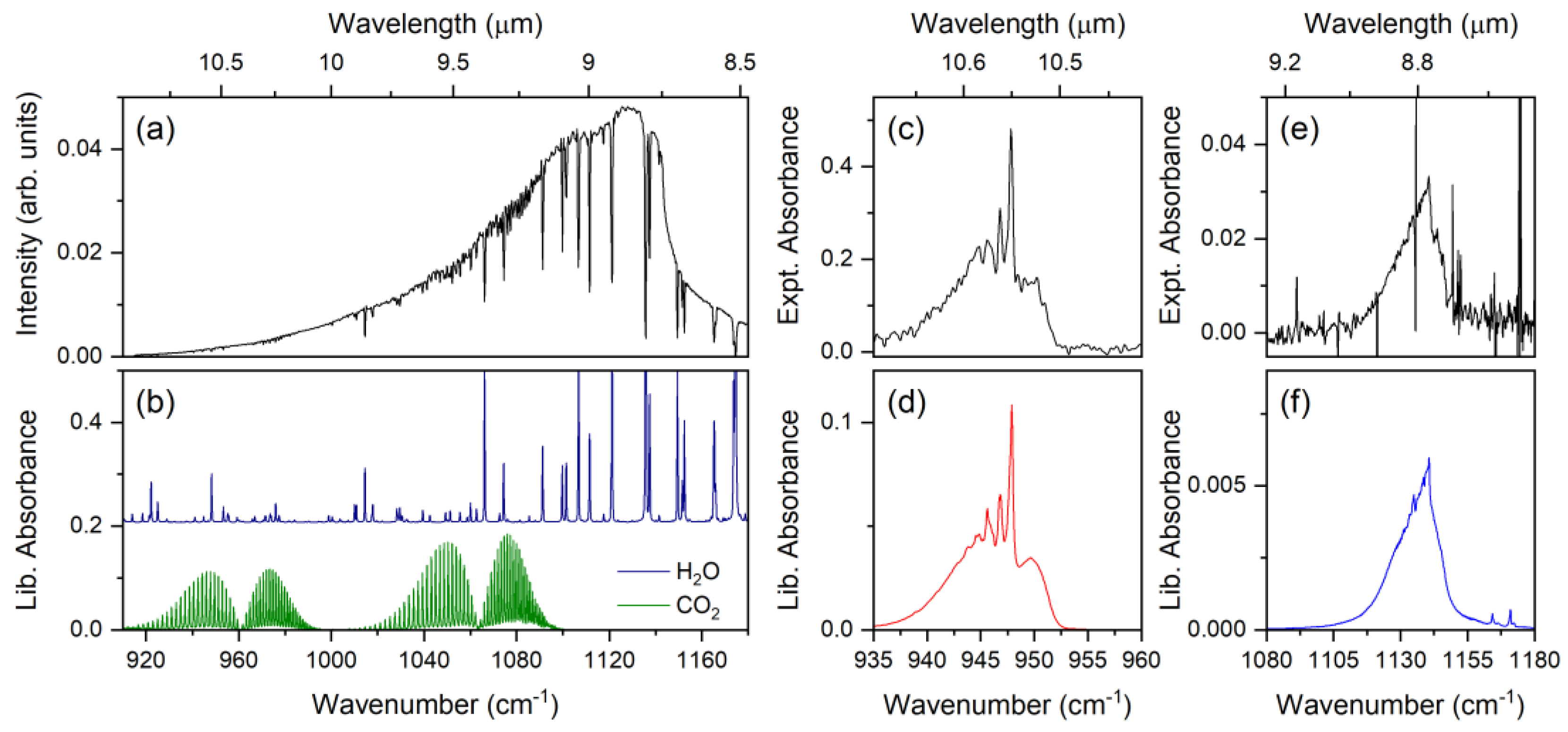


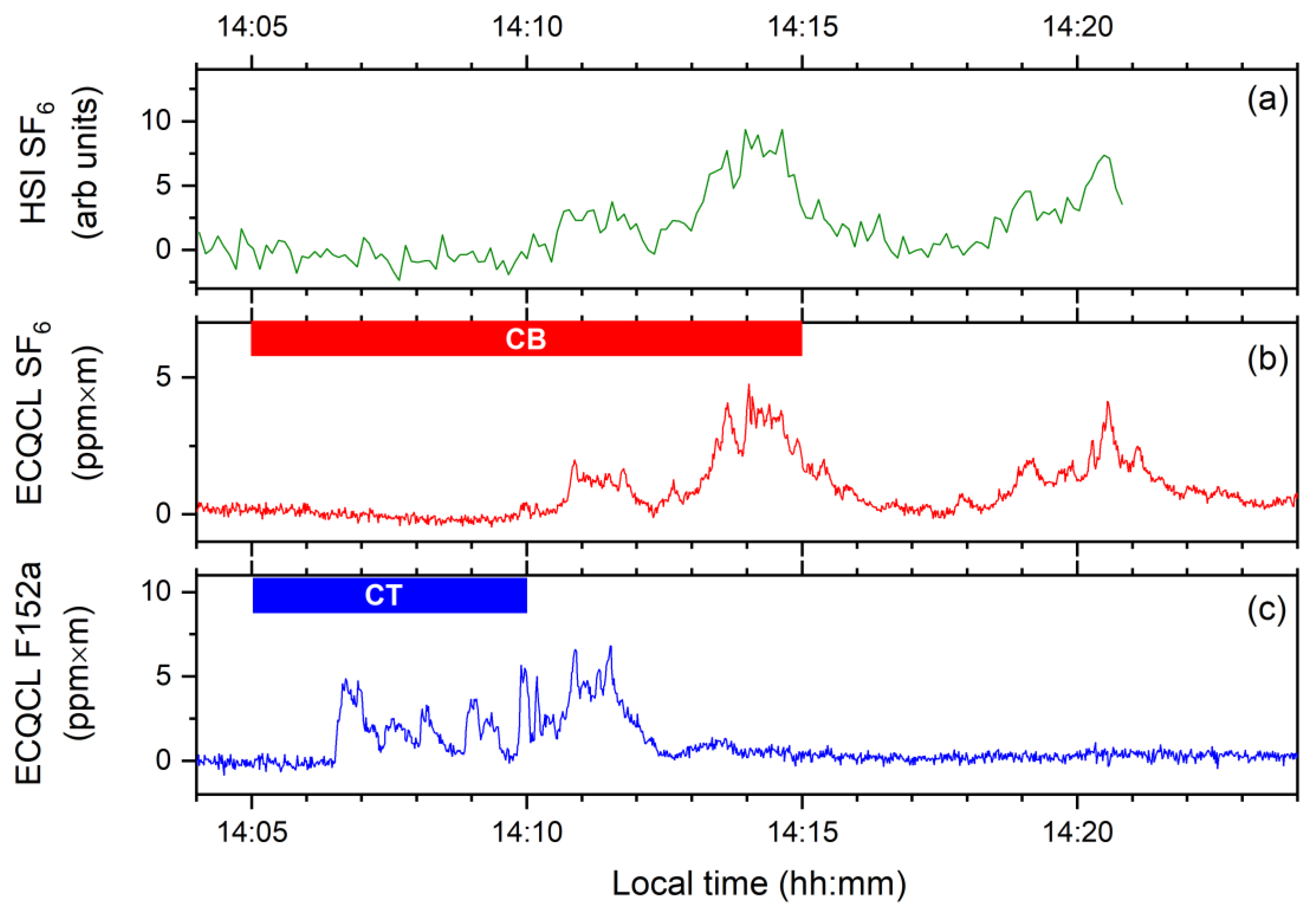
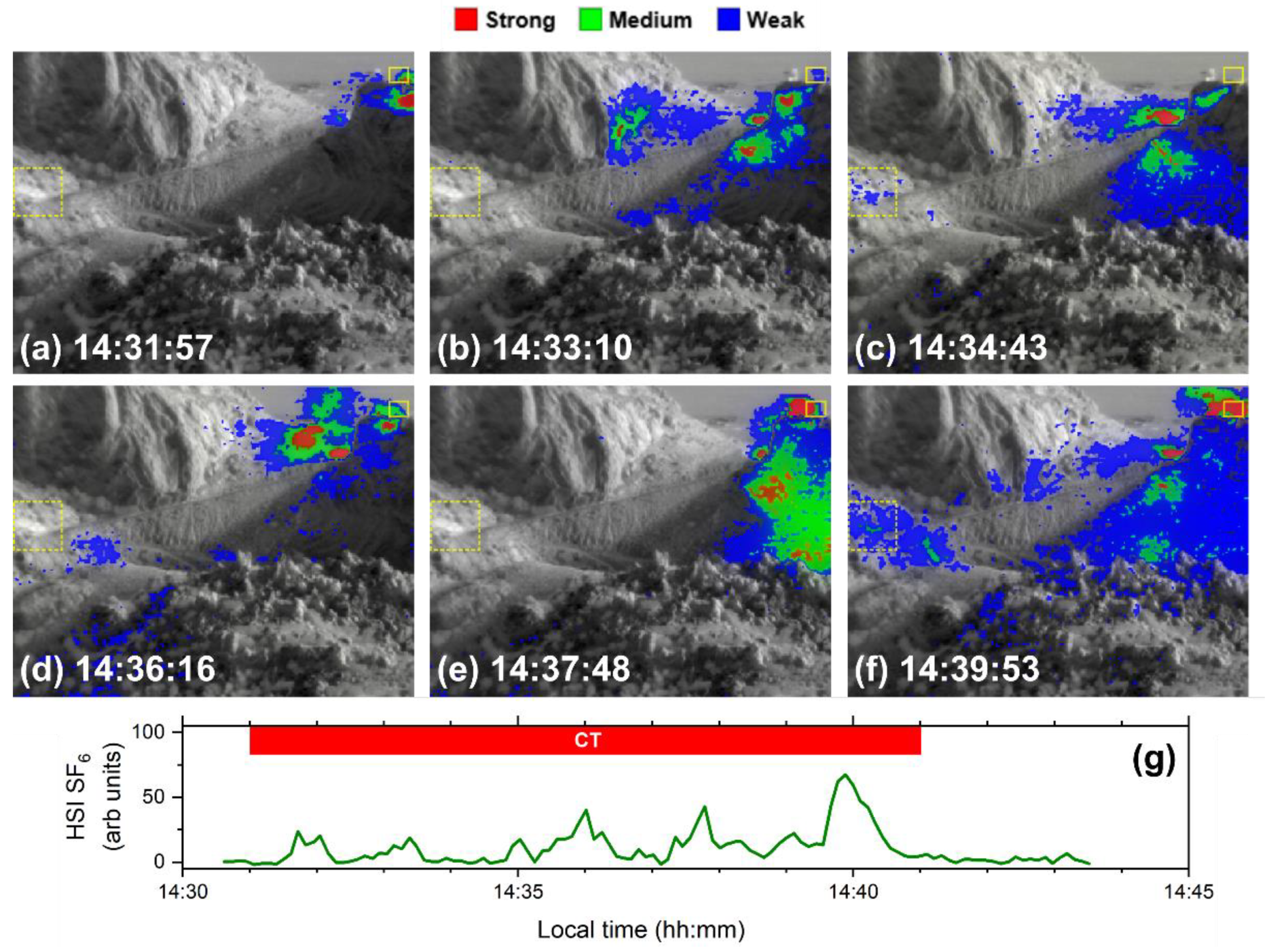
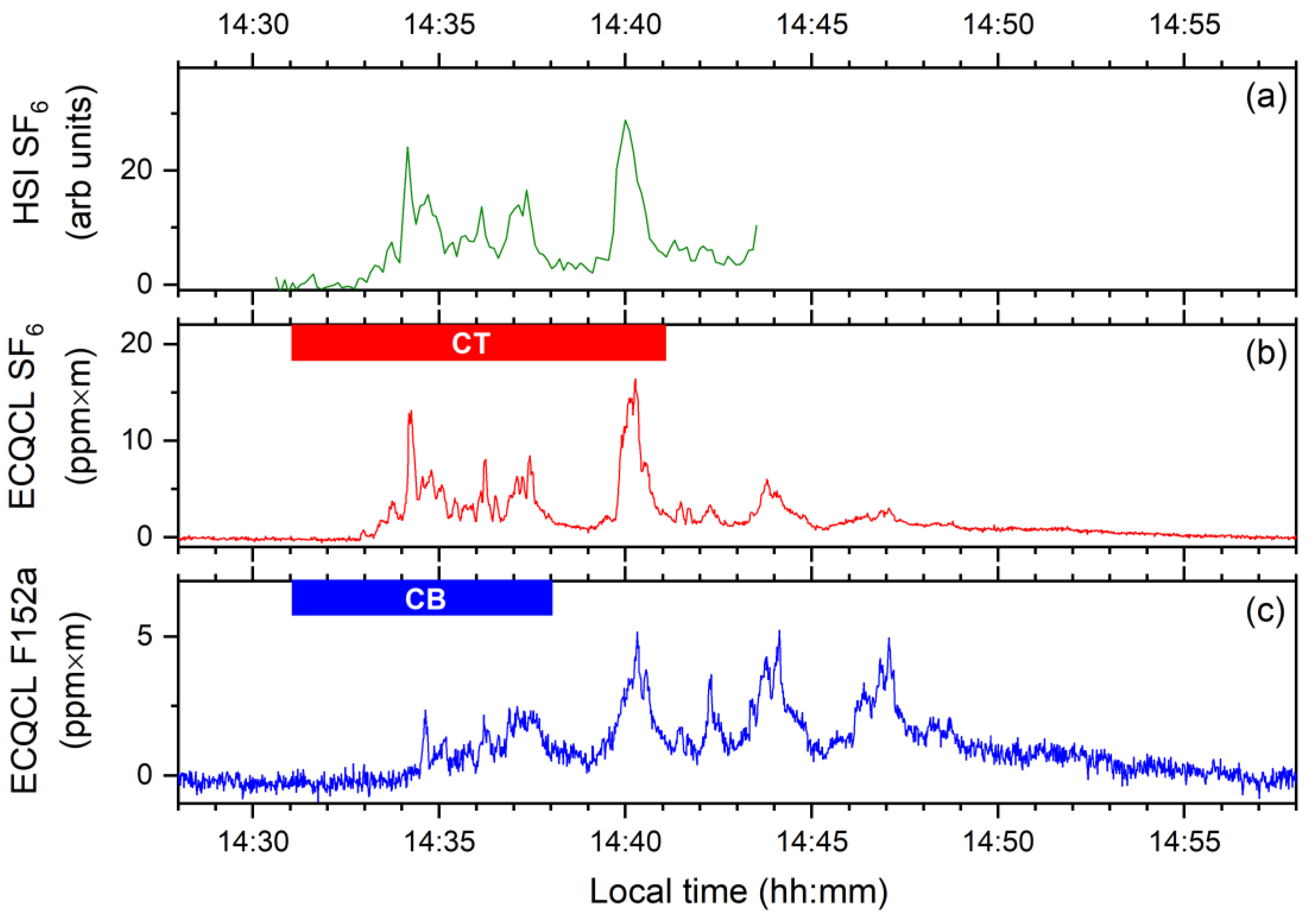

Publisher’s Note: MDPI stays neutral with regard to jurisdictional claims in published maps and institutional affiliations. |
© 2022 by the authors. Licensee MDPI, Basel, Switzerland. This article is an open access article distributed under the terms and conditions of the Creative Commons Attribution (CC BY) license (https://creativecommons.org/licenses/by/4.0/).