Article

Relationship between Urban Three-Dimensional Spatial Structure and Population Distribution: A Case Study of Kunming’s Main Urban District, China

1
Faculty of Geography, Yunnan Normal University, Kunming 650500, China
2
Guangzhou Institute of Geography, Guangdong Academy of Sciences, Guangzhou 510070, China
3
School of Architecture and Urban Planning, Guangdong University of Technology, Guangzhou 510090, China
*
Author to whom correspondence should be addressed.
Remote Sens. 2022, 14(15), 3757; https://doi.org/10.3390/rs14153757
Submission received: 28 June 2022 / Revised: 28 July 2022 / Accepted: 3 August 2022 / Published: 5 August 2022

Abstract

:
The three-dimensional (3D) spatial structure within cities can reveal more information about land development than the two-dimensional spatial structure. Studying the relationship between the urban 3D spatial structure and the population distribution is a crucial aspect of the relationship between people and land within cities. However, a few relevant studies focus on the differences between employment population and night population distribution in relation to urban 3D spatial structure. Therefore, this study proposes a new concept of 3D space-filling degree (3DSFD), which is applicable to evaluate the city’s 3D spatial structure. We took 439 blocks in Kunming’s Main Urban District as a sample and analyzed the 3D spatial structure based on geographic information data at the scale of a single building. The characteristics and differences of the daytime and night population distribution in Kunming’s Main Urban District were identified using cell phone signaling big data. Accordingly, a cross-sectional dataset of the relationship between the city’s 3D spatial structure and the population distribution was constructed, with the 3D space-filling degree of the block as the dependent variable, two indicators of population distribution (daytime and night population density) as the explanatory variables, and seven indicators of distance from the city center, and building, road, and functional place densities, proportion of undevelopable land area, housing prices, and land use type as the control variables. We used spatial regression models to explore the significance, strength, and direction of the relationship between urban 3D spatial structure and population distribution. We found that the spatial error model (SEM) was the most effective. The results show that only night population distribution is significantly and positively related to 3DSFD. Every 1% increase in night population density in a block will increase the value of 3DSFD by 2.8307%. The night population distribution is the core factor affecting the 3D spatial structure of Kunming’s Main Urban District. The correlation between daytime population distribution and 3DSFD is not significant. This variability has been ignored in previous studies. The findings are informative for further understanding of the relationship between urban 3D space and population distribution, especially the difference between night and daytime populations. This study can help city managers reasonably plan urban land development intensity and construction height, guide the population layout and formulate management policies to improve urban population and space matching, enhancing the livability and attractiveness of cities.

1. Introduction

The three-dimensional (3D) spatial structure within cities is an important perspective to show the urban land use status [1]. The rapid development of remote sensing and geographic information technologies gradually makes the 3D basic data of cities abundant, making it possible to study the 3D spatial structure within cities. Compared with the traditional study of the two-dimensional (2D) spatial structure of urban land, the 3D spatial structure can show more information about land development. For example, it can indicate the spatial characteristics of the intensity and scope of urban land development [2,3,4,5]. In contrast, the 2D spatial structure can only characterize the development density (e.g., building density) [6]. Therefore, it is necessary to conduct relevant studies on the characteristics of 3D spatial structures within cities. There are many ways to evaluate the inner city across three dimensions, such as floor area ratio, building coverage ratio, building shape coefficient, total building volume, spatial congestion degree, and so on [7,8]. Further, how to properly evaluate urban 3D space and thus accurately describe the 3D spatial structure of the city is a topic worth exploring because its evaluation is more complex than for 2D spaces. For example, the volume ratio is commonly used to describe the 3D spatial structure [9,10,11,12,13]. Still, the volume ratio is closely related to the number of building stories [14,15] but cannot fully reflect the building height [16]. The spatial congestion degree (SCD) evaluates space crowding, but the denominator of the SCD indicator (plot volume) is influenced by the average building height of the plot. The average building height varies between plots, which makes plots of different building heights not cross-sectionally comparable. Therefore, a reasonably usable index for evaluating urban 3D spatial structure is needed.
A classic urban geography research topic is the relationship between urban spatial structure and population distribution. Many studies have explored the correspondence between urban development density [17,18,19], development pattern [20,21], land-use properties [22], urban population distribution, and other factors. For example, these factors such as urban land use [23,24,25], built environment [26,27,28,29], urban morphology [30,31,32], public service accessibility [33,34], urban functional space, building density [35,36], and road density [37] are the relationship between urban 2D spatial structure and population distribution [38,39,40]. In contrast, research to recognize and understand the relationship between 3D urban spatial structure and urban population distribution is important. Theoretically, the relationship between 3D space and population distribution should be closer than that between a 2D space and population distribution. This is because the higher the intensity of urban agglomeration, the higher the intensity of urban development, and the more likely it is that cities will expand to “higher altitudes.” Current research on the relationship between 3D urban spatial structure and population distribution has focused on the relationship between these indicators and population distribution from the perspectives of building height, building density, building volume, floor area ratio, and spatial congestion. In terms of building height, Alahmadi used land cover and height data for the remote sensing of the building, to estimate the spatial distribution of the population in Riyadh, Saudi Arabia, showing a strong positive correlation between building height and population distribution [41]; Yu et al. studied the potential of 3D building height data in terms of socio-economic activity characteristics, and the results showed that 3D building height information has great potential to support various studies in the urban domain, such as population distribution and carbon emissions [42]. In terms of building density, typical studies include Yao et al., who mapped fine-scale population distribution at the building level by integrating multi-source geospatial big data, where building scale was used to map population distribution [43]; Zhu et al. suggested that population distribution was related to building size [44]. In terms of building volume, more typical studies include that of Zhao et al.’s, whose results show that the relationship between building volume and population is more non-stationary and positively correlated in household-oriented and mixed-use blocks [45]; Qiu et al. confirmed that building volume is a more valuable indicator and estimator of block-level population distribution, demonstrating a high correlation [46]. In terms of floor area ratio, Kono et al. [47] concluded that floor area ratio is positively correlated with population distribution. Zeng et al. found that the floor–area ratio is a positive factor for population clustering, using the central city of Tianjin as an example [35]. Tan et al. concluded that population distribution is the main determinant of floor area ratio [48]. This shows that urban 3D space is closely related to population distribution.
However, urban population distribution is dynamic [25,49], i.e., the population distribution pattern differs somewhat during daytime and night. During the daytime, when employment occurs, the urban population distribution is characterized by the employment-population distribution. Conversely, at night, when most residents are at home, the urban population distribution is characterized by the night population distribution. Thus, it is necessary to distinguish the variability of the relationship between the daytime and night population and the 3D spatial structure of the city. In existing studies on urban 3D spaces and population distribution, the population is often treated as static, with little attention paid to this variability. To fill this gap, we subdivided the population distribution into daytime and night population and investigate the variability of the daytime population distribution and night population distribution concerning the 3D spatial structure separately. Further, we tried to identify: (1) Whether both daytime and night population distribution are closely related to the 3D spatial structure and (2) Which category of the daytime and night population has the greatest influence on the 3D spatial structure, and what is the direction and intensity of that influence? This is where this study goes further than extant research, and this is the main goal of this study. The theoretical value of this study lies in it examining the relationship between population distribution and urban 3D space from the perspective of dynamic population distribution (distinguishing between daytime and night population). The practical significance of this study lies in the fact that the dynamic distribution of population distinguishes between the employment and residence of residents in the 3D spatial structure of the city, which in turn provides theoretical support for the formulation of planning policies for urban employment space and residential space.
Kunming is an important city in southwest China. Its main urban area has diverse land types, high building densities, large differences in development intensity, and a rich urban skyline, forming a diverse 3D urban spatial structure with large differences. Furthermore, Kunming’s Main Urban District is the most dominant location for population concentration, with a high population density. More importantly, there is a large difference in the distribution of daytime and night population in Kunming’s Main Urban District. According to this study, the total daytime population of Kunming’s Main Urban District is 3,256,000, while the total night population is only 2,621,000, with the daytime population exceeding the night population by 635,000. This characteristic makes the city suitable as a case city for this study.
Therefore, this study proposes a concept applicable to evaluating the urban 3D spatial structure of different plots within cities, explores the relationship between urban 3D spatial structure and population distribution, and distinguishes the differences between daytime population distribution and 3D spatial structure and night population distribution and 3D spatial structure. Specifically, taking 439 blocks in Kunming’s Main Urban District as an example, we construct a new concept for evaluating the 3D space utilization of parcels (blocks)—3D space filling degree (3DSFD), and based on which the 3D spatial structure of Kunming’s Main Urban District is studied. We use cell phone signaling big data to identify the characteristics of daytime and night population distribution in Kunming’s Main Urban District. Based on this, we constructed the cross-sectional dataset of the daytime population density (DPD), night population density (NPD), distance from the city center (DFCC), building density (BD), road density (RD), functional place density (FPD), proportion of undevelopable land area (ULA), housing prices (HP), and land use type (LUP). We used spatial regression models to explore the relationship between daytime and night population distributions and the 3D spatial filling of the plots, including the degree and direction of correlation. This has innovative value in terms of research ideas and research perspectives. This study will help city managers reasonably plan urban land development intensity and construction height, and distinguish between land development policies for employment and residential spaces. In addition to this, it can also guide the population layout and formulate management policies to improve urban population and space matching and enhance the livability and attractiveness of cities.
The rest of this study is structured as follows. In the second section, this study proposes the concepts of 3DSFD and population distribution, evaluation methods, research framework, index system, and data sources. The third section shows the spatial pattern of 3D spatial structure and population distribution in the main urban area of Kunming. It then analyzes the degree and direction of the population distribution’s influence on 3D spatial structure. Finally, the research results are discussed, and conclusions are drawn.

2. Materials and Methods

2.1. Concept and Calculation Method of 3D Space-Filling Degree

There are many ways to evaluate the inner city across three dimensions, among which spatial congestion degree (SCD) is a calculated index to evaluate space crowding [7,8]. The SCD is the volume of buildings on a plot divided by the volume of the plot (determined by the average height of the buildings), which considers both the volume of the buildings and the plot. However, the denominator of the SCD indicator (plot volume) is influenced by the average building height of the plot. The average building height varies between plots, which makes plots of different building heights not horizontally comparable. This is because the volumes of the high-rise building plots are scaled up, while the volumes of the low-rise building plots are reduced. Therefore, based on the evaluation idea of SCD, we fixed the height of the plots so that the volume of the plots is only influenced by the area of the plots, which makes them more comparable between different plots. In this way of thinking, we established a new concept—3D space filling degree—to evaluate the 3D space utilization of a plot. This is different from the traditional concept of floor area ratio and the SCD mentioned above. This is because the floor ratio area is related to the building density and the number of building stories, while the 3DSFD constructed in this study is related to the building height and the number of building stories. Generally, different types of buildings have different floor heights. For example, the floor height of industrial buildings is higher than that of residential buildings. If the floor area ratio is used to evaluate the 3D space utilization of a plot, the height information is not accurately reflected. The 3DSFD within an arbitrary parcel of land with a given base height can be defined as the ratio of building volume to parcel volume. The unit is %. Suppose a plot has only one building A, then the 3DSFD of the plot can be expressed as:
3 D S F D P = V A / V P × 100 %
where VA is the volume of building A and VP is the volume of the plot P. The volume of plot P is determined by the plot’s area SP and base height LP. The base height LP can be set freely according to the actual research needs, and when multiple parcels are compared, the base height LP needs to be unified. Thus, the 3DSFD can be further expressed as:
3 D S F D P = S A × L A S P × L P × 100 %
In reality, a plot often includes multiple buildings. If the plot has n buildings, then the 3DSFD of the plot can be expressed as:
3 D S F D P = i = 1 n S i × L i S P × L P × 100 %
where i is the building number and n is the total number of buildings on the site.
Therefore, the value of 3DSFD ranges from 0 to 100%. The higher the value, the higher the intensity of 3D space utilization of the site. Ceteris paribus, the 3DSFD is proportional to the total building area, average building height, and number of buildings, respectively. Meanwhile, 3DSFD is inversely proportional to the parcel’s area and base height. Therefore, the 3DSFD can be used to evaluate the difference in 3D space utilization intensity of different plots within the city.

2.2. Concept and Evaluation Methods of Urban Population Distribution

Urban population distribution is often dynamic. During the day, the population distribution during working hours and the population distribution at night (residence) is different because residents do not necessarily work (or go to school, same below) and live in the same location. The daytime population distribution is based on the population distribution between 9:00 and 18:00 on weekdays, because this time of day is the main activity time for most residents (working hours); the night population distribution is based on the population distribution between 21:00 and 7:00 a.m. the following day (regardless of weekdays and holidays), because this is the time when most residents rest at night in their residences (nighttime). We then used the population density to represent the distribution of the city population. Then, the daytime population density (DPD) of plot p can be expressed as:
D P D P = D P P / S P
where DPP is the number of the daytime population in plot p, and SP is plot p area. The night population density of plot p is expressed as:
N P D P = N P P / S P
where NPP is the number of people living in plot p.

2.3. Research Area

Kunming is a megacity in southwest China and the capital of Yunnan Province. The area enclosed by Kunming’s Third Ring Road can be regarded as the city’s main urban area, our study area. The Third Ring Road consists of the following roads: North Third Ring, Golden Avenue, Yuanbo, East Third Ring, Changhong, Guangfu, Huayuan, Chunyu, and West Third Ring. The main urban area of Kunming is the city’s core and most important area, with an area of 140.45 km2. The study area is divided into the old area, core area, and urban district (Figure 1) according to the main urban district’s first and second ring roads. A total of 439 blocks were used as the basic study unit. The intersection of Youth Road and Renmin Middle Road in the old area can be regarded as Kunming’s urban center.

2.4. Research Design, Indicator System, and Model

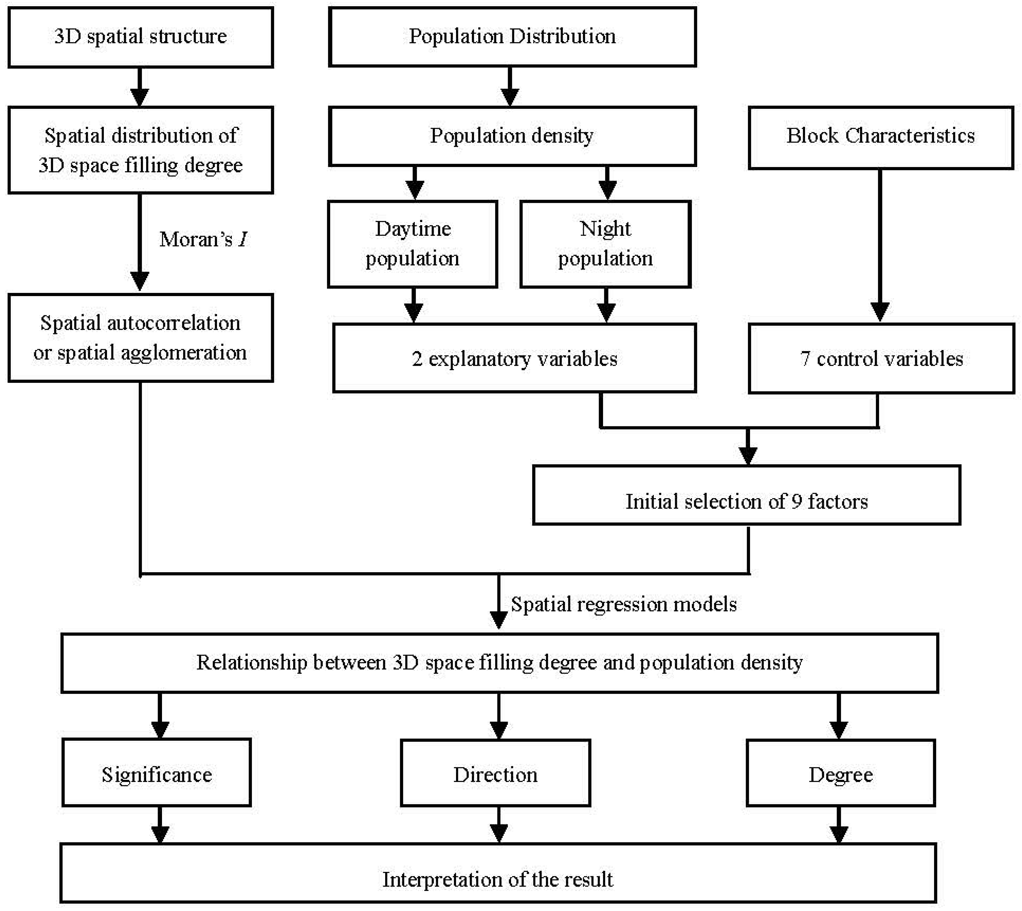
This study constructed a research framework to analyze the relationship between the 3D spatial structure and city population distribution. The analysis process is as follows. First, 439 blocks in Kunming’s Main Urban District were used as the research object to analyze the spatial distribution and spatial correlation characteristics of the 3D spatial filling degree of the city. Second, we analyzed the spatial distribution characteristics of daytime and night population densities in Kunming’s Main Urban District and the differences between them. Third, the influencing-factors model of 3DSFD was constructed, including DPD, NPD, DFCC, BD, RD, FPD, PULA, HP, and LUP. The explanatory variables were DPD and NPD, and DFCC, BD, RD, FPD, PULA, HP, and LUP were control variables. Fourth, the relationship between urban 3DSFD and population density (including DPD and NPD) was analyzed by selecting the appropriate model among OLS, spatial lag model (SLM), and spatial error model (SEM). This relationship included the significance, direction, and intensity of influence. Finally, the research results were analyzed (Figure 2).
See Table 1 for a system of factors and indicators of urban 3D space-filling.
Among them, proportion of undevelopable land area (PULA) was calculated by taking the proportion of water, green space, and forest area in each block; HP was derived by calculating the mean value of the average listed price of all residential quarters in each block. For the variable of LUP, as different land use types have different impacts on the 3DSFD, we assigned different scores (1–5) to different land use types. The score was assigned as follows: 5 for business offices land, 4 for residential and commercial services land, 3 for industrial and warehousing, administrative, educational, and medical services land, 2 for transport stations, sports and culture land, and 1 for roads, parks and green spaces. The score was then weighted by the proportion of each type of land in the block to calculate the score for each type of land in the block and finally aggregated to give a score for each type of land use in the block.
According to Table 1, we construct a model to analyze the relationship between 3D spatial structure and population distribution in Kunming’s main urban area. The model is represented as.
3 D S F D = f ( D P D ,   N P D , D F C C , B D , R D , F P D ,   P U L A ,   H P , L U P )
where 3DSFD is the 3D space filling degree, which is the model’s dependent variable, indicating the block’s 3D space utilization status. DPD and NPD represent the explanatory variables for daytime and night population densities, respectively. The existing population density distribution is an important factor to consider in the decision-making process of urban 3D spatial development. Therefore, developers in densely populated areas are more likely to conduct high-intensity land development, resulting in a higher 3D spatial filling degree. For example, Koziatek et al. argue that population density is a key criterion for determining the optimal location for vertical development of mid-rise buildings [22]; Biljecki et al. also argue that building height is correlated with population density because taller buildings can accommodate more people [50]. DFCC, BD, RD, FPD, PULA, HP, and LUP are control variables. Ding and Lin (2019) found that building height in cities is more sensitive to distance from the city center [51,52]. Theoretically, the higher the BD, the higher the intensity of urban 3D space utilization in cities. RD is a manifestation of urban transportation convenience, and areas with developed transportation are more densely built with more high-rise buildings. FPD reflects the transportation accessibility, attractiveness of business, and convenience of work and life and governs the spatial distribution of the building mix. Lin and Sun et al. considered that the density of functional places such as employment places, commercial and service places, public facilities, and subway stations is an important factor influencing the height of urban buildings [52,53]. Theoretically, the higher the proportion of ULA in a block, the stronger the building space constraint in that block and the more difficult it is to develop, so the smaller the 3D space filling degree; the higher the HP, the higher the development value of the land, the better the location, the easier it is for developers to carry out high-intensity development, so theoretically the larger the 3D space infill; and different LUP have different effects on 3D spatial filling degree. Business office land tends to have a higher 3D space filling degree, followed by residential and commercial services land. The 3DSFD is even lower for industrial and warehousing, administration, educational, and medical services, transport stations, sports and cultural land, and lowest for roads, parks, and green spaces.

2.5. Data and Data Sources

The attribute data of the 3D building outline and its building height were obtained from the “Baidu Map”, and the data was collected in February 2021. The population distribution data is obtained from “iZone Data” (provided by Shenzhen Hexun Huagu Information Technology Co., Ltd.), based on cell phone signaling data analysis. The “iZone Data” was collected for a period of three months, from 1 April to 30 June 2021. Addresses with the highest frequency between 21:00 and 7:00 during this period were defined as nighttime population locations. Location Based Services (LBS) data has limitations and does not provide an accurate picture of population distribution. For example, it is difficult for LBS to count the location of users who do not use mobile phones or related mobile location devices. However, mobile phone usage is currently very high in China, therefore using LBS data to estimate the changing characteristics of population distribution within cities at different times of the day is the most appropriate and feasible way to conduct urban research with the current level of technology. The original data provided were 200m* 200m grid data. We converted the scale of the data by the spatial matching method and have the grid data converted to block-scale data. Among them, the daytime population distribution is based on the population distribution from 9:00 to 18:00 on weekdays; the night population distribution is based on the population distribution from 21:00 to 7:00 a.m. the next day (regardless of weekdays and holidays). The DFCC was calculated based on the distance of the block center from the city center. The city center is at the intersection of Youth Road and People’s Middle Road. BD and RD were calculated based on floor area and road length data (from “Baidu Maps”). FPD was calculated from the number of functional places, including employment places (office buildings, government agencies, and social organizations, companies and enterprises, financial and insurance services), commercial service places density (catering services, shopping services, living services), public service places (scientific, educational and cultural services, health care services, sports and leisure services), and public transportation facilities density (subway stations and bus stops). The data of Functional place was obtained from AMAP POI, and the data collection period is in January 2021. The water and green space vector data required for PULA were obtained from Baidu Map; the residential quarter location data were obtained from Baidu Map in February 2021, and the average listed price data were mainly obtained from Anjuke (https://km.anjuke.com/, accessed on 18 November 2021 ) in November 2021, supplemented by the Baidu website (https://www.baidu.com/, accessed on 16 December 2021 ); the land use type data were obtained by referring to Gong et al. [54], and data were downloaded from Esstsinghua (http://data.ess.tsinghua.edu.cn/, accessed on 9 August 2020), data dated 2018.

2.6. Spatial Regression Model

To study the relationship between urban 3D spatial structure and population distribution in the main urban area of Kunming, we constructed a model of factors influencing the intensity of urban 3D spatial utilization. The model takes urban 3D spatial utilization intensity (with 3DSFD as the evaluation index) as the dependent variable, the two population density indicators in Table 1 as the explanatory variables (independent variables), and the seven indicators of block characteristics in Table 1 as the control variables. Ordinary least squares regression model (OLS), SLM, and SEM were used to calculate and select the optimal model to analyze the relationship between 3DSFD and population density in Kunming and then analyze the relationship between urban 3D spatial structure and population distribution.
The OLS model can analyze the linear relationship between 3DSFD and the nine influencing factors. However, the model does not account for the spatial interactions of blocks. Therefore, the OLS model expression is as follows.
y i = β X i + ε i , [   ε i ~ N ( 0 ,   δ 2 I ) ]
where i = 1, 2, …, 439, is the block (basic study unit) of the main urban area of Kunming; yi is 3DSFD in the block; Xi is the S-dimensional row vector (s = 1, 2, …, 9) of 3DSFD influencing factor, representing the value of the s-th influencing factor variable in the i-th block; β is the S-dimensional column vector, being the regression coefficient; ε is the error term of the model, εi~N(0,δ2I) denotes that the error term follows a normal distribution and the variance is consistent, where I is the unit matrix.
The SLM accounts for the spatial interactions between blocks and is a form of a spatial regression model. The SLM can be expressed as [55,56].
y i = ρ j = 1 n W i j y j + β X i + ε i ,   [   ε i ~ N ( 0 ,   δ 2 I ) ]
where ρ stands for the coefficient value of spatial autoregressive; Wij is spatial weight matrix.
The SEM model is suitable for analyzing the possible spatial spillover effects of independent error terms. The SEM model can be expressed as [55,57].
y i = λ j = 1 n W i j φ j + β X i + ε i ,   [   ε i ~ N ( 0 ,   δ 2 I ) ]
where ϕ denotes the spatial autocorrelation error term s is the model of factors influencing the intensity of urban 3D space utilization, and λ is the spatial autocorrelation coefficient of the error term.

3. Results

3.1. Urban 3D Spatial Structure

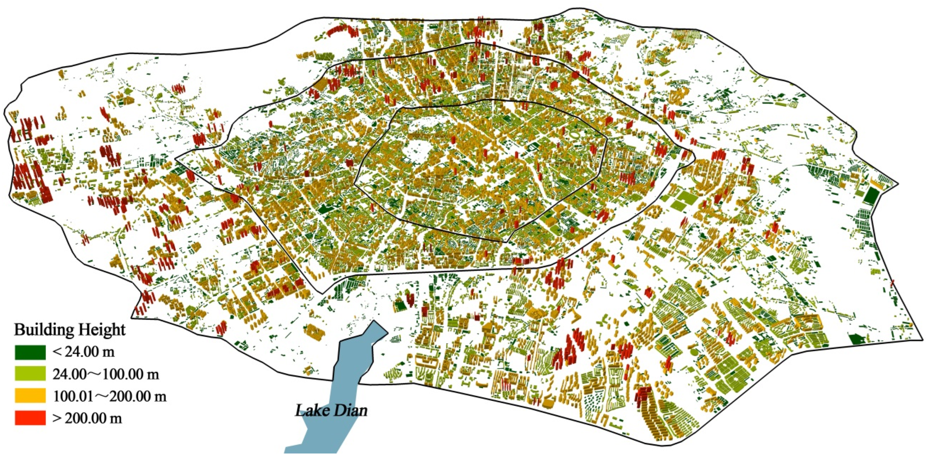
Figure 3 shows the 3D spatial pattern of single building scales in Kunming’s Main Urban District. The figure shows that buildings over 200 m are mainly distributed outside the second ring road (urban district), while the number of buildings over 200 m in the old area is less. However, regarding building density, the building density inside the second ring road (old area and core area) is much higher than that outside the second ring road (urban district).
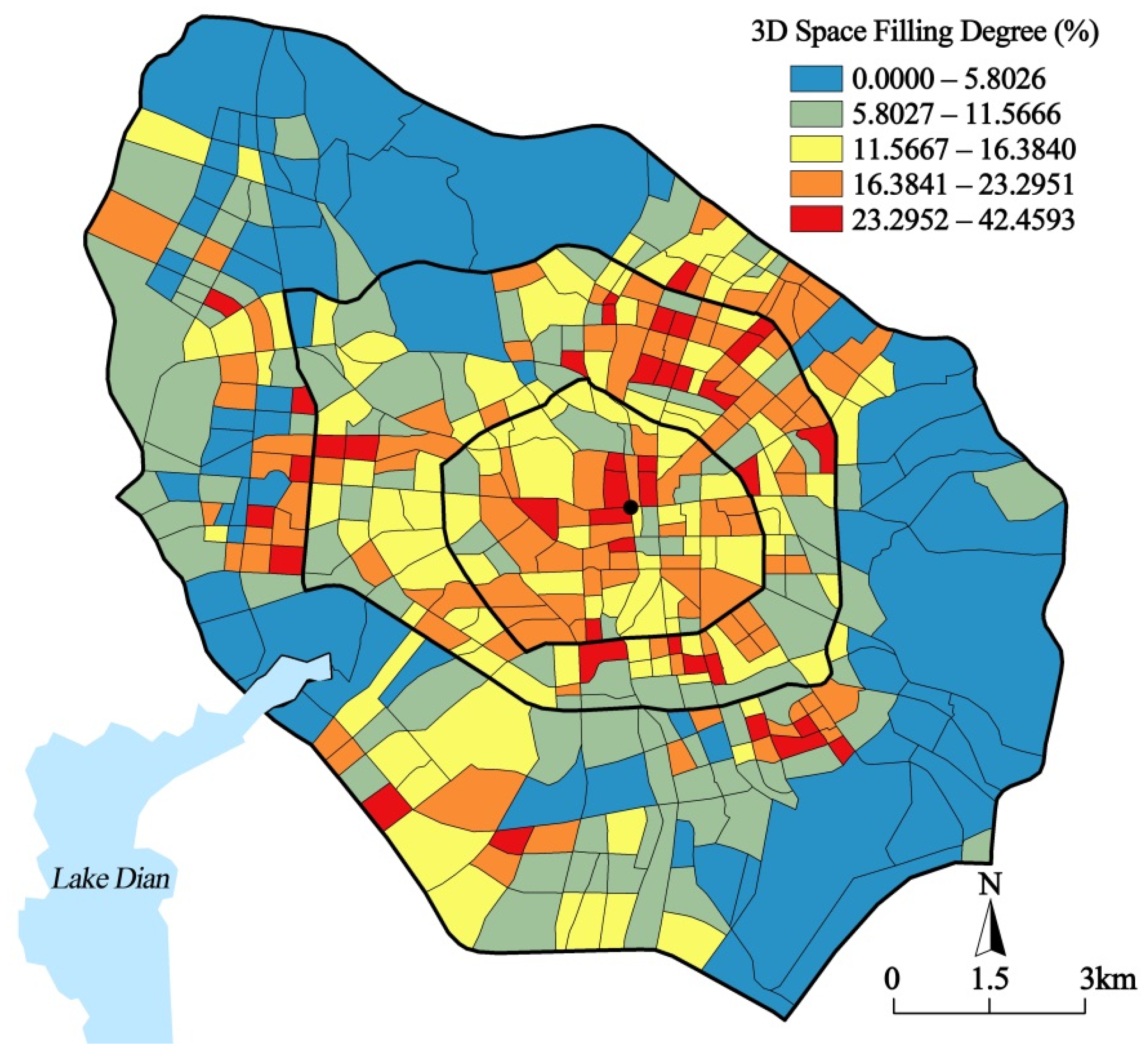
Based on this data, the block-scale 3DSFD was calculated. Figure 4 shows the descriptive statistics of 3DSFD. We divided 5 data intervals: 0.0000–5.8026%, 5.8027–11.5666%, 11.5667–16.3840%, 16.3841–23.2951%, and 23.2952–42.4593%. The number of communities in each interval is 69, 109, 113, 109, and 39, respectively.
Figure 5 shows the spatial distribution pattern of 3DSFD in Kunming’s Main Urban District based on ArcGIS 10.0. The block with 3DSFD lower than 5.8026% is located outside the second ring road (urban district). However, the block with 3DSFD higher than 23.2952% is mainly located in the center of the old area (near the city center), north of the core area, and west and southeast of the urban district.
Moran’s I index was used to analyze the spatial autocorrelation characteristics of 3DSFD in 439 blocks in Kunming’s Main Urban District. The fixed distance method was used to determine the spatial interrelationship and was set to 1000 m. The results showed that the Moran’s I index was 0.2483, the p-value was 0.0000, and the z-statistic value was 13.9047, indicating that the 3DSFDs in Kunming’s Main Urban District showed significant spatial correlation characteristics. That is, the 3DSFD of a certain block will be influenced by the neighboring blocks.

3.2. Spatial Pattern of Population Distribution

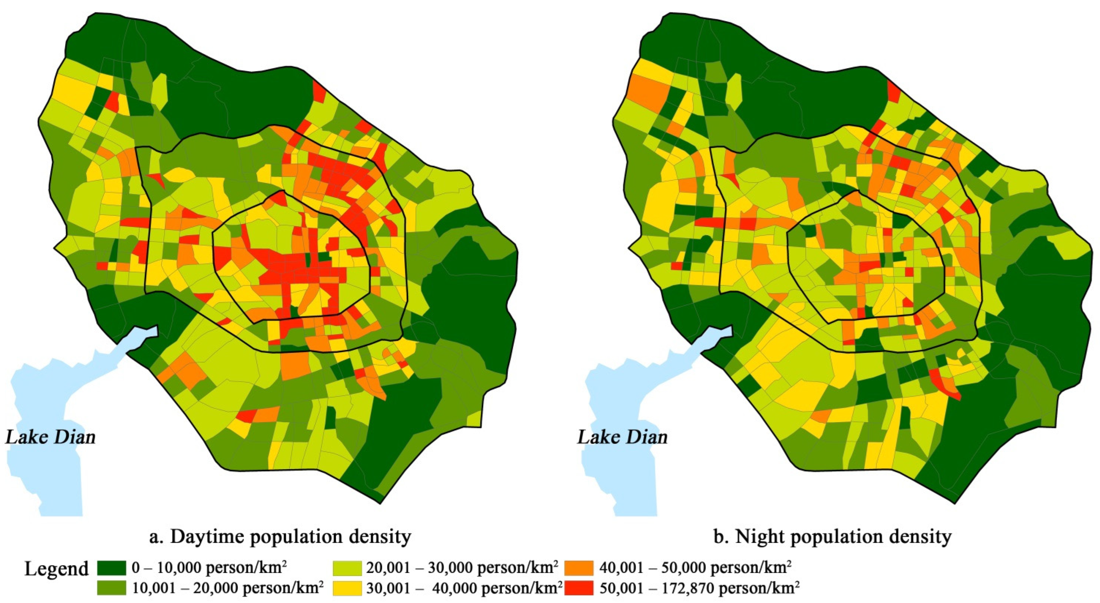
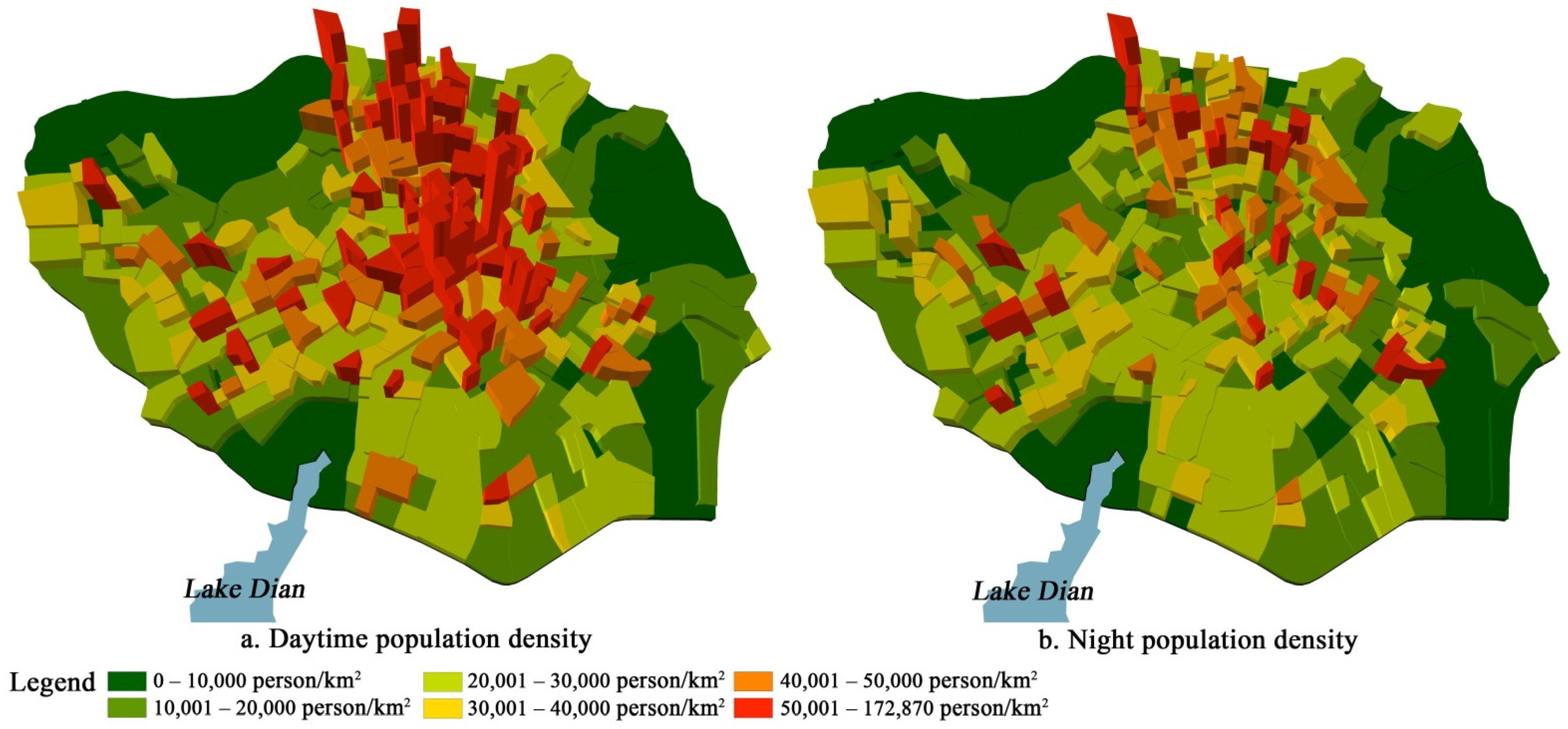
As this study area is Kunming’s Main Urban District, it tends to be the employment catchment area, and there will be more DPD than NPD. The total employed population in the study area is 3,256,000 and is 635,000 more than the total residential population of 2,621,000. This is consistent with Kunming’s Main Urban District as the main employment location. Regarding the overall population density of the study area, the DPD is 23,182 people/km2, and the NPD is 18,661 people/km2. We used 10,000, 20,000, 30,000, 40,000, and 50,000 people/km2 as the thresholds for the block population density divisions to form six population intervals and then GIS to draw the spatial DPD and NPD of Kunming’s Main Urban District distribution pattern (Figure 6). Additionally, the ArcScene program was used to draw the 3D spatial distribution map of DPD and NPD (Figure 7). These maps show that the number of blocks with DPD higher than 50,000 persons/km2 is much higher than that of NPD. The blocks with DPD higher than 50,000 persons/km2 are located in the center of the old city and the northeast of the core area. The blocks with DPD lower than 20,000 persons/km2 are mainly located northwest of the core and urban areas. The blocks with NPD higher than 50,000 persons/km2 are fewer in number, and the blocks with NPD lower than 20,000 persons/km2 are fewer. The blocks with NPD below 20,000 persons/km2 are located in the urban district, the northwestern part of the core area, and the periphery of the old area. The population distribution pattern of DPD and NPD differ.

3.3. Relationship between Urban 3D Spatial Structure and Population Distribution in Kunming’s Main Urban District

First, the nine impact factors of 3DSFD were tested for covariance (Table 2). The test results showed that the VIF values of all nine indicators were lower than 10, indicating no significant cointegration among these nine factors. Therefore, all of them could be included in the regression model.
Three regression methods, OLS, SLM, and SEM, were used to analyze the relationship between urban 3D spatial structure and population distribution. The results (Table 3) show that among the OLS, SLM, and SEM models, the SEM model has the largest R2 of 0.546415 and the lowest AIC value of 2664.95. Thus, the SEM seems to fit significantly better than the other two models. Further, we performed an LM test to determine the best spatial regression model. The results show that Lagrange Multiplier (SEM) has a significant p-value of 0.0001, which is more significant than Lagrange Multiplier (SLM) (p-value of 0.0933). We also performed statistical tests for the robustness of both spatial regression models. The robust LM test shows that SEM has a significant p-value of 0.0001, significant at the 0.01 level, and the Robust LM test for SLM was not significant. Combining these aspects, the SEM is most suitable for explaining the 3D spatial structure and population distribution. Table 4 shows the results of the SEM model.
To verify the accuracy of the results, we conducted significance F-tests and robustness tests on the model. First, based on the R2 value of the SEM model results, we calculated the F-test value to be 57.4221; here, the significance level α was defined as 0.05, and by consulting the F-test critical value distribution table, we know that Fα is 1.902, and the F value is greater than the critical value (F> Fα), indicating that the model passes the F test and the model is significant. Further, the model was tested for robustness in three different ways: by comparing the results of different models, by changing the number of control variables to the model and by constructing different weights. Firstly, we compared the regression results of the OLS and SEM models, and the results showed that NPD had a significant positive effect on 3DSFD, while DPD did not have a significant effect on 3DSFD, and the explanatory variables were significant in the same direction of influence in both models. Similarly, we also compared the SLM model with the SEM model results and the results were the same; Secondly, we regressed the model again after reducing three additional control variables (that is, PULA, HA, and LUP) to the original seven control variables, and the results showed that the SEM results were optimal, and the explanatory variables (DPD and NPD) were significant and consistent in the direction of influence across both models. Thirdly, we used the three methods of fixed distance, queen, and rook to construct different weights, and for the fixed distance method, we set the distance threshold to 1500 m and 2000 m, respectively, and ran the regression model based on the four newly constructed weights and compared them. The results of these three robustness tests indicate that the model is significant and robust, which also indicates that the model results are accurate.
Based on the significance of the regression coefficients, the relationship between 3D spatial structure and population distribution can be judged. Table 4 shows that among the two population distribution indicators, NPD has a significant effect on 3DSFD, while DPD is not significant. This indicates that among the population distributions, night population distribution is the core factor influencing the 3D spatial structure of Kunming’s Main Urban District. In contrast, the daytime population distribution influence is not significant. For NPD, every 1% increase in night population density in the block will increase the value of 3DSFD by 2.8307%. Therefore, there is a significant positive correlation between them.
Additionally, for the control variables, at the 0.01 level, BD had a significant positive effect on 3DSFD; at the 0.05 level, FPD, PULA, and LUP all had varying degrees of effect on 3DSFD. For BD, for every 1% increase, the value of 3DSFD will increase by 4.5480%. This indicates that BD is a significant determinant of 3DSFD. For FPD, the value of 3DSFD will increase by 0.9073% for every 1% increase. This indicates that the denser the blocks in the city’s functional place, the greater the 3DSFD. For PULA and LUP, for every 1% increase in PULA, the 3DSFD value decreases by 0.5323%, while for every 1% increase in LUP, the 3DSFD value increases by 2.9564%. This indicates that the larger the PULA, that is, the smaller the proportion of developable land in the block, the smaller the 3DSFD value; however, the larger the LUP, that is, the more the land type in the block can support high-intensity land development, the higher the 3DSFD value. In general, the results are in line with the theoretical expectations. In contrast, DFCC, RD, and HP have no significant effects on 3DSFD.
As the SEM model was used in this study, the influence of the independent variables of the surrounding parcels (e.g., population distribution) on the independent variables of the parcel was considered in the modeling technique by including the measurement equation in the form of a spatial error term. The results of this study show that the SEM model gives better results than the OLS and SLM models, suggesting that there is a spatial spillover effect of the population distribution on the 3DSFD. Of course, not only does the population distribution have a spatial spillover effect, but the control variables selected in this study also have a spatial spillover effect. Therefore, the spatial spillover effect must be considered when studying the influence of intra-city population distribution on the 3D spatial structure.

4. Discussion and Conclusions

4.1. Discussion

This study proposes a new concept for evaluating the 3D space utilization of a plot (block), 3DSFD. Compared with the traditional concept of floor area ratio, the 3DSFD proposed in this study is more suitable for describing a city’s 3D spatial structure. Its advantage is that it can reflect the influence of the difference in floor height of different building types. For example, the 3DSFD of industrial land is often larger than the 3DSFD value of residential land in the same area and plot ratio. Unfortunately, the academic community has paid little attention to this phenomenon. In addition, the 3DSFD is better suited than the existing spatial congestion degree for estimating (comparing) differences in the degree of development of different plots‘ 3D space. This is because the denominator (plot volume) in the SCD index is influenced by the average building height of the plot. The 3DSFD proposed in this paper fixes the height of the plot, making it possible to directly compare the 3D spatial development degree of different plots. Therefore, the concept of 3DSFD proposed in this study can be used to evaluate when describing the cities’ 3D spatial structure in the future.
Taking Kunming’s Main Urban District as an example, we analyzed the relationship between 3D spatial structure and population distribution, especially distinguishing between daytime population (working population) distribution and night population (residential population) distribution. The results show that the night population distribution is significantly and positively correlated with the 3DSFD. This indicates that the formation of 3D spatial structure in Kunming’s Main Urban District is dominated by residential buildings rather than office or commercial buildings. This is because residential buildings have a better match with the night population. In recent years, most of the new residential buildings in Kunming have been high-rise buildings and developed with high intensity. As a result, the number of high-rise buildings of residential type buildings is higher than that of office and commercial buildings. It indicates that residential development is the core driving force in shaping the 3D spatial structure of Kunming’s Main Urban District.
A conclusion that differs from some of the traditional and obvious findings [41,42,43,44,45,46] is that the daytime population distribution does not explain the 3D spatial structure very well. The reason for this may be that the uncontrolled overdevelopment of office and commercial buildings in Kunming, where the number of developments far exceeded the office and commercial demand, did not bring in more employment to the city, thereby resulting in a higher vacancy rate of office and commercial buildings in the city. This makes the relationship between 3D spatial structure and daytime population distribution insignificant, which is a novel finding from this study.
It is notable that the relationship between 3DSFD and the population distribution is spatially heterogeneous. The significance, direction, and strength of the relationship between 3DSFD and population distribution may vary at different regional locations. This effect is not considered in this study, which is a shortcoming. The spatial differences of livability factors can be further analyzed by geographically weighted regression in the future. Secondly, there may be differences in the relationship between 3DSFD and population distribution for different land use types. The differences in the results for different land use types can be studied in the future through segmentation studies. Thirdly, the use of blocks as the basic research unit is still rather rough, and in the future, more refined research units (e.g. residential quarters, buildings) could be used for research.

4.2. Conclusions

The 3DSFD can be used as a basic evaluation unit regarding parcels or blocks. Furthermore, the higher the value of 3DSFD, the higher the intensity of 3D space utilization. Therefore, the 3DSFD can describe the difference in 3D space utilization intensity within the city.
The 3D spatial structure of Kunming’s Main Urban District is reflected by the fact that the areas with high 3DSFD are concentrated in the center of the old area (near the city center), the northern part of the core area, and the western and southeastern parts of the urban district. Some areas outside the second ring road (urban district) have lower 3DSFD. The 3DSFD of Kunming’s Main Urban District shows significant spatial correlation characteristics, and the neighboring blocks influence the 3DSFD of a block. Therefore, the population distribution characteristics of DPD and NPD differ in population distribution patterns.
This study used SEM to analyze the relationship between urban 3D spatial structure and population distribution (daytime and night population) and its significance. The results show that only the night population distribution is significantly and positively correlated with the 3DSFD. For every 1% increase in night population density in a block, the value of 3DSFD will increase by 2.8307%. The night population distribution is the core factor affecting the 3D spatial structure of Kunming’s Main Urban District. The correlation between daytime population distribution and 3DSFD is not significant.

4.3. Policy Implications

The findings of this study can provide decision support for the spatial planning of cities in the following ways: (1) When planning the development intensity of urban plots, it is necessary to use not only floor area ratio, building density and building height as control indicators, but also 3DSFD as control indicators. (2) Government departments should use the spatially differentiated characteristics and changing trends of population distribution as an important basis for guiding the development intensity of land parcels. A differentiated 3D spatial planning strategy can be adopted for plots of land across different urban location conditions. In areas with high population distribution density, the intensity of 3D spatial development should be appropriately increased so that the building supply can meet the demand for population use. In areas with low population density, the development intensity of plots should be strictly controlled, with a lower intensity of 3D spatial development as far as possible, to avoid vacant buildings. (3) In areas with low daytime population distribution, excessive office and commercial buildings should be avoided, and the scale of office and commercial land use should be reduced by adjusting the type of land use through planning means, and the intensity of development of office and commercial buildings should be reduced. (4) When preparing spatial planning schemes, spatial planners should analyze the relationship between the 3D spatial structure of the city and the distribution of the daytime and nighttime population, and use the characteristics of this relationship as an important reference for the preparation of spatial planning schemes. (5) It is recommended that government departments prepare a special 3D spatial plan for the city and make this special plan an important element of the spatial planning content system.

Author Contributions

Conceptualization, Y.W. and C.L.; methodology, Y.W.; software, X.Y.; validation, X.Y., M.W. and C.L.; formal analysis, Y.W.; investigation, Y.W.; resources, Y.W.; data curation, Y.W.; writing—original draft preparation, Y.W., X.Y. and M.W.; writing—review and editing, Y.W., Y.S.; visualization, Y.W. and X.Y.; supervision, Y.W., H.Z.; project administration, Y.W., C.L., H.Z. and Y.S.; funding acquisition, Y.W. and H.Z. All authors have read and agreed to the published version of the manuscript.

Funding

This research was funded by the National Natural Science Foundation of China (No. 41871150), GDAS Special Project of Science and Technology Development (No. 2020GDASYL-20200104001; 2020GDASYL-20200102002), Key Program of the National Natural Science Foundation of China (No.42130712), Special Construction Project of Guangdong–Hong Kong–Macao Greater Bay Area Strategic Research Institute (No. 2021GDASYL-20210401001).

Data Availability Statement

Not applicable.

Acknowledgments

We would like to thank two reviewers for constructive comments and insightful suggestions that have greatly improve the quality of the manuscripts.

Conflicts of Interest

The authors declare no conflict of interest.

References

  1. Xia, F.Z.; Shen, Y.; Yan, J.M.; Bao, H.X.H. On the potential of urban three-dimensional space development: The case of Liuzhou, China. Habitat Int. 2016, 51, 48–58. [Google Scholar] [CrossRef]
  2. Peng, J.; Liu, Q.H.; Blaschke, T.; Zhang, Z.; Liu, Y.X.; Hu, Y.N.; Wang, M.; Xu, Z.H.; Wu, J.S. Integrating land development size, pattern, and density to identify urban-rural fringe in a metropolitan region. Landsc. Ecol. 2020, 35, 2045–2059. [Google Scholar] [CrossRef]
  3. Zhang, W.P.; Shi, P.J.; Tong, H.L. Research on construction land use benefit and the coupling coordination relationship based on a three-dimensional frame model—A case study in the Lanzhou-Xining urban agglomeration. Land 2022, 11, 460. [Google Scholar] [CrossRef]
  4. Koziatek, O.; Dragicevic, S. A local and regional spatial index for measuring three-dimensional urban compactness growth. Environ. Plan. B-Urban Anal. City Sci. 2019, 46, 143–164. [Google Scholar] [CrossRef]
  5. Wei, Y.G.; Huang, C.; Lam, P.T.I.; Yuan, Z.Y. Sustainable urban development: A review on urban carrying capacity assessment. Habitat Int. 2015, 46, 64–71. [Google Scholar] [CrossRef]
  6. Gao, S.H.; Zhan, Q.M.; Yang, C.; Liu, H.M. The diversified impacts of urban morphology on land surface temperature among urban functional zones. Int. J. Environ. Res. Public Health 2020, 17, 9578. [Google Scholar] [CrossRef]
  7. Xu, X.; Ou, J.; Liu, P.; Liu, X.P.; Zhang, H.H. Investigating the impacts of three-dimensional spatial structures on CO2 emissions at the urban scale. Sci. Total Environ. 2021, 762, 143096. [Google Scholar] [CrossRef]
  8. Lin, J.Y.; Lu, S.Y.; He, X.Y.; Wang, F. Analyzing the impact of three-dimensional building structure on CO2 emissions based on random forest regression. Energy 2021, 236, 121502. [Google Scholar] [CrossRef]
  9. Yin, C.; Yuan, M.; Lu, Y.; Huang, Y.; Liu, Y. Effects of urban form on the urban heat island effect based on spatial regression model. Sci. Total Environ. 2018, 634, 696–704. [Google Scholar] [CrossRef]
  10. Qiao, W.F.; Gao, J.B.; Guo, Y.Z.; Ji, Q.Q.; Wu, J.; Cao, M. Multi-dimensional expansion of urban space through the lens of land use: The case study of Nanjing City, China. J. Geogr. Sci. 2019, 29, 749–761. [Google Scholar] [CrossRef] [Green Version]
  11. Wang, H.B.; Cai, M.; Yao, Y.F. A modified 3D algorithm for road traffic noise attenuation calculations in large urban areas. J. Environ. Manag. 2017, 196, 614–626. [Google Scholar] [CrossRef] [PubMed]
  12. Zheng, Z.; Zhou, W.Q.; Wang, J.; Hu, X.F.; Qian, Y.G. Sixty-year changes in residential landscapes in Beijing: A perspective from both the horizontal (2D) and vertical (3D) dimensions. Remote Sens. 2017, 9, 992. [Google Scholar] [CrossRef] [Green Version]
  13. Zhou, W.Q.; Wang, J.; Cadenasso, M.L. Effects of the spatial configuration of trees on urban heat mitigation: A comparative study. Remote Sens. Environ. 2017, 195, 1–12. [Google Scholar] [CrossRef]
  14. Li, X.M.; Zhang, D.H.; Tian, S.Z.; Wang, M. Spatial and temporal differences of urban residential quarter floor area ratio: A case study of four districts in Dalian. Sci. Geogr. Sin. 2018, 38, 531–538. [Google Scholar]
  15. Lee, J.M.; Braham, W. Right-sizing cities for maximum power: Urban form parameters for New York City and the Greater Philadelphia Region. Sustainability 2019, 11, 2352. [Google Scholar] [CrossRef] [Green Version]
  16. Usui, H. Building height distribution under zoning regulations: Theoretical derivation based on allometric scaling analysis and application to harmonise building heights. Environ. Plan. B-Urban Anal. City Sci. 2021, 48, 2520–2535. [Google Scholar] [CrossRef]
  17. Rao, Y.; Zhou, J.; Zhou, M.; He, Q.S.; Wu, J.Y. Comparisons of three-dimensional urban forms in different urban expansion types: 58 sample cities in China. Growth Chang. 2020, 51, 1766–1783. [Google Scholar] [CrossRef]
  18. He, S.J.; Wang, X.Y.; Dong, J.R.; Wei, B.C.; Duan, H.M.; Jiao, J.Z.; Xie, Y.W. Three-dimensional urban expansion analysis of valley-type cities: A case study of Chengguan district, Lanzhou, China. Sustainability 2019, 11, 5663. [Google Scholar] [CrossRef] [Green Version]
  19. Jayasinghe, A.; Madusanka, N.B.S.; Abenayake, C.; Mahanama, P.K.S. A modeling framework: To analyze the relationship between accessibility, land use and densities in urban areas. Sustainability 2021, 13, 467. [Google Scholar] [CrossRef]
  20. Zhao, S.C.; Liu, Y.; Liang, S.; Wang, C.; Arora, M. Effects of urban forms on energy consumption of water supply in China. J. Clean. Prod. 2020, 253, 119960. [Google Scholar] [CrossRef]
  21. Dong, T.; Jiao, L.M.; Xu, G.; Liu, J.F. Towards sustainability? Analyzing changing urban form patterns in the United States, Europe, and China. Sci. Total Environ. 2019, 671, 632–643. [Google Scholar] [CrossRef] [PubMed]
  22. Koziatek, O.; Dragićević, S. iCity 3D: A geosimualtion method and tool for three-dimensional modeling of vertical urban development. Landsc. Urban Plan. 2017, 167, 356–367. [Google Scholar] [CrossRef]
  23. Zuo, T.; Wei, H.; Liu, H.; Yang, Y.J. Bi-level optimization approach for configuring population and employment distributions with minimized vehicle travel demand. J. Transp. Geogr. 2019, 74, 161–172. [Google Scholar] [CrossRef]
  24. Peng, Y.; Liu, J.; Zhang, T.; Li, X. The Relationship between urban population density distribution and land use in Guangzhou, China: A spatial spillover perspective. Int. J. Environ. Res. Public Health 2021, 18, 12160. [Google Scholar] [CrossRef]
  25. Li, J.G.; Li, J.W.; Yuan, Y.; Li, G.F. Spatiotemporal distribution characteristics and mechanism analysis of urban population density: A case of Xi’an, Shaanxi, China. Cities 2019, 86, 62–70. [Google Scholar] [CrossRef]
  26. Li, Z.H.; Jiao, L.M.; Zhang, B.E.; Liu, J.F. Understanding the pattern and mechanism of spatial concentration of urban land use, population and economic activities: A case study in Wuhan, China. Geo-Spatial Inf. Sci. 2021, 24, 678–694. [Google Scholar] [CrossRef]
  27. Joshi, K.K.; Kono, T. Optimization of floor area ratio regulation in a growing city. Reg. Sci. Urban Econ. 2009, 39, 502–511. [Google Scholar] [CrossRef]
  28. Koohsari, M.J.; Badland, H.; Giles-Corti, B. (Re)Designing the built environment to support physical activity: Bringing public health back into urban design and planning. Cities 2013, 35, 294–298. [Google Scholar] [CrossRef]
  29. Salgado, M.; Madureira, J.; Mendes, A.S.; Torres, A.; Teixeira, J.P.; Oliveira, M.D. Environmental determinants of population health in urban settings. A systematic review. BMC Public Health 2020, 20, 853. [Google Scholar] [CrossRef]
  30. Liu, Y.; Wang, F.; Xiao, Y.; Gao, S. Urban land uses and traffic source-sink areas: Evidence from GPS-enabled taxi data in Shanghai. Landscape Urban Plan. 2012, 106, 73–87. [Google Scholar] [CrossRef]
  31. Pei, T.; Sobolevsky, S.; Ratti, C.; Shaw, S.L.; Li, T.; Zhou, C. A new insight into land use classification based on aggregated mobile phone data. Int. J. Geogr. Inf. Sci. 2014, 28, 1988–2007. [Google Scholar] [CrossRef] [Green Version]
  32. Louail, T.; Lenormand, M.; Cantu Ros, O.G.; Picornell, M.; Herranz, R.; Frias-Martinez, E.; Ramasco, J.J.; Barthelemy, M. From mobile phone data to the spatial structure of cities. Sci. Rep. 2014, 4, 5276. [Google Scholar] [CrossRef] [PubMed] [Green Version]
  33. Song, Y.; Tan, Y.; Song, Y.; Wu, P.; Cheng, J.C.P.; Kim, M.J.; Wang, X. Spatial and temporal variations of spatial population accessibility to public hospitals: A case study of rural-urban comparison. Gisci. Remote Sens. 2018, 55, 718–744. [Google Scholar] [CrossRef]
  34. Lan, F.; Gong, X.; Da, H.; Wen, H. How do population inflow and social infrastructure affect urban vitality? Evidence from 35 large- and medium-sized cities in China. Cities 2020, 100, 102454. [Google Scholar] [CrossRef]
  35. Zeng, P.; Sun, Z.Y.; Chen, Y.Q.; Qiao, Z.; Cai, L.W. COVID-19: A comparative study of population aggregation patterns in the Central Urban Area of Tianjin, China. Int. J. Environ. Res. Public Health 2021, 18, 2135. [Google Scholar] [CrossRef] [PubMed]
  36. Dovey, K.; Pafka, E. The urban density assemblage: Modelling multiple measures. Urban Design Int. 2014, 19, 66–76. [Google Scholar] [CrossRef]
  37. Shi, G.; Shan, J.; Ding, L.; Ye, P.; Li, Y.; Jiang, N. Urban road network expansion and its driving variables: A case study of Nanjing City. Int. J. Environ. Res. Public Health 2019, 16, 2318. [Google Scholar] [CrossRef] [Green Version]
  38. Liu, G.; Yao, X.B.; Luo, Z.M.; Kang, S.W.; Long, W.; Fan, Q.J.; Gao, P.C. Agglomeration centrality to examine spatial scaling law in cities. Comput. Environ. Urban Syst. 2019, 77, 10. [Google Scholar] [CrossRef]
  39. Sakamoto, K.; Iida, A.; Yokohari, M. Spatial patterns of population turnover in a Japanese Regional City for urban regeneration against population decline: Is Compact City policy effective? Cities 2018, 81, 230–241. [Google Scholar] [CrossRef]
  40. Tsai, Y.H. Quantifying urban form: Compactness versus ‘Sprawl’. Urban Stud. 2016, 42, 141–161. [Google Scholar] [CrossRef]
  41. Alahmadi, M.; Atkinson, P.; Martin, D. Estimating the spatial distribution of the population of Riyadh, Saudi Arabia using remotely sensed built land cover and height data. Comput. Environ. Urban Syst. 2013, 41, 167–176. [Google Scholar] [CrossRef]
  42. Yu, G.J.; Xie, Z.X.; Li, X.C.; Wang, Y.X.; Huang, J.X.; Yao, X.C. The potential of 3-D building height data to characterize socioeconomic activities: A case study from 38 cities in China. Remote Sens. 2022, 14, 2087. [Google Scholar] [CrossRef]
  43. Yao, Y.; Chen, W.Z.; Chen, X.D.; Yu, J.S. Mapping fine-scale population distributions at the building level by integrating multisource geospatial big data. Int. J. Geogr. Inf. Sci. 2017, 31, 1220–1244. [Google Scholar] [CrossRef]
  44. Zhu, S.N.; Dai, Q.; Zhao, B.R.; Shao, J.Q. Assessment of population exposure to urban flood at the building scale. Water 2020, 12, 3253. [Google Scholar] [CrossRef]
  45. Zhao, Y.; Ovando-Montejo, G.A.; Frazier, A.E.; Mathews, A.J.; Flynn, K.C.; Ellis, E.A. Estimating work and home population using LIDAR-derived building volumes. Int. J. Remote Sens. 2017, 38, 1180–1196. [Google Scholar] [CrossRef]
  46. Qiu, F.; Sridharan, H.; Chun, Y. Spatial autoregressive model for population estimation at the census block level using LiDAR−derived building volume information. Cartogr. Geogr. Inf. Sci. 2010, 37, 239–257. [Google Scholar] [CrossRef]
  47. Kono, T.; Kaneko, T.; Morisugi, H. Necessity of minimum floor area ratio regulation: A second-best policy. Ann. Reg. Sci. 2010, 44, 523–539. [Google Scholar] [CrossRef]
  48. Tan, S.K.; Liu, Q.; Han, S.Y. Spatial-temporal evolution of coupling relationship between land development intensity and resources environment carrying capacity in China. J. Environ. Manag. 2022, 301, 113778. [Google Scholar] [CrossRef]
  49. Zhong, W.; Wang, D.; Xie, D.; Yan, L. Dynamic characteristics of Shanghai’s population distribution using cell phone signaling data. Geogr. Res. 2017, 36, 972–984. [Google Scholar]
  50. Biljecki, F.; Arroyo Ohori, K.; Ledoux, H.; Peters, R.; Stoter, J. Population estimation using a 3D city model: A multi-scale country-wide study in the Netherlands. PLoS ONE 2016, 11, e0156808. [Google Scholar] [CrossRef]
  51. Ding, C. Building height restrictions, land development and economic costs. Land Use Pol. 2013, 30, 485–495. [Google Scholar] [CrossRef]
  52. Lin, J.; Wan, H.; Cui, Y. Analyzing the spatial factors related to the distributions of building heights in urban areas: A comparative case study in Guangzhou and Shenzhen. Sust. Cities Soc. 2020, 52, 101854. [Google Scholar] [CrossRef]
  53. Sun, W.; Li, T. Building height trends and their influencing factors under China’s rapid urbanization: A case study of Guangzhou, 1960–2017. Chin. Geogr. Sci. 2020, 30, 993–1004. [Google Scholar] [CrossRef]
  54. Gong, P.; Chen, B.; Li, X.; Liu, H.; Wang, J.; Bai, Y.; Chen, J.; Chen, X.; Fang, L.; Feng, S.; et al. Mapping essential urban land use categories in China (EULUC-China): Preliminary results for 2018. Sci. Bull. 2019, 65, 182–187. [Google Scholar] [CrossRef] [Green Version]
  55. Anselin, L. Spatial Econometrics: Methods and Models; Springer: Dordrecht, The Netherlands, 1988; pp. 1–254. [Google Scholar]
  56. Anselin, L.; Syabri, I.; Kho, Y. GeoDa: An introduction to spatial data analysis. Geogr. Anal. 2006, 38, 5–22. [Google Scholar] [CrossRef]
  57. Arbia, G. Spatial Econometrics: Statistical Foundations and Applications to Regional Economic Growth; Springer: Berlin/Heidelberg, Germany, 2006; pp. 1–146. [Google Scholar]
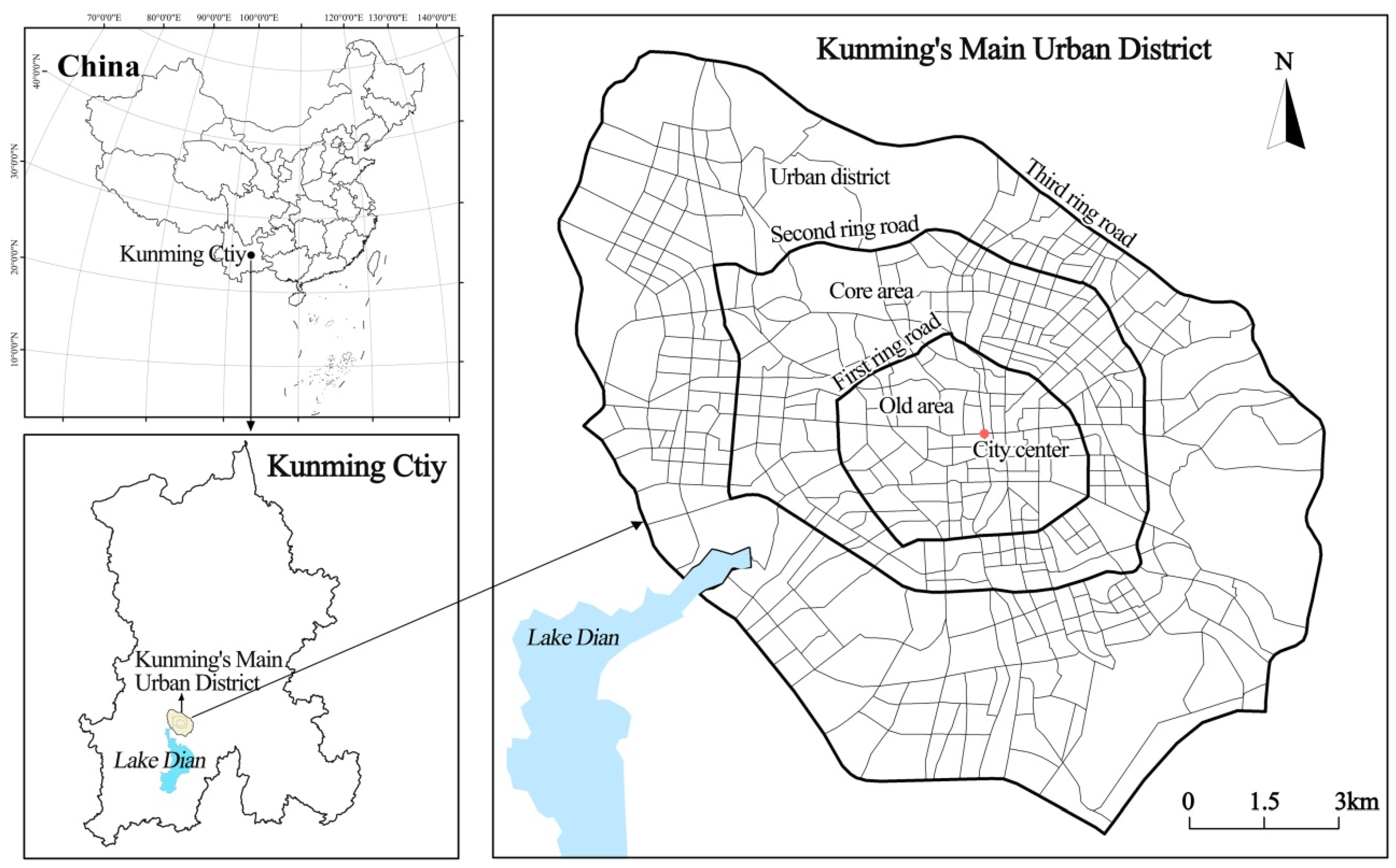
Figure 1. Study area.
Remotesensing 14 03757 g001
Figure 2. Research design.
Remotesensing 14 03757 g002
Figure 3. 3D spatial pattern distribution of single buildings in Kunming’s Main Urban District.
Remotesensing 14 03757 g003
Figure 4. Descriptive statistics of 3DSFD in Kunming’s Main Urban District by blocks.
Remotesensing 14 03757 g004
Figure 5. The spatial distribution pattern of 3DSFD in Kunming’s Main Urban District using the natural breaks (Jenks) method.
Remotesensing 14 03757 g005
Figure 6. The spatial difference pattern of population density in Kunming’s Main Urban District.
Remotesensing 14 03757 g006
Figure 7. The 3D spatial difference pattern of population density in Kunming’s Main Urban District.
Remotesensing 14 03757 g007
Table 1. Definitions and evaluation methods for the variables.
Variable (Symbol)UnitExpected Impact Direction
Dependent Variable
3D space filling degree (3DSFD)%
Explanatory Variables—Population Density
Daytime population density (DPD)Person/km2+
Night population density (NPD)Person/km2+
Control Variables—Block Characteristics
Distance from the city center (DFCC)m+
Building density (BD)%+
Road density (RD)km/km2+
Functional place density (FPD)Point/km2+
Proportion of undevelopable land area (ULA)%-
Housing prices(HP)Yuan/m2+
Land use type(LUP)Score+
Table 2. The collinearity test of impact factors of 3DSFD in Kunming’s Main Urban District.
ToleranceVIF Value
DPD0.1715.833
NPD0.2005.002
DFCC0.5481.826
BD0.3752.668
RD0.8231.215
FPD0.3263.066
PULA0.9341.071
HP0.8361.196
LUP0.8921.121
Table 3. Comparison of the OLS, SLM, and SEM models.
ModelR2AICLog Likelihood
OLS0.5180412683.99−1332.00
SLM0.5247012681.01−1329.50
SEM0.5464152664.95−1322.48
Table 4. SEM model results.
CoefficientStd. Errort/z-Valuep
DPD−1.22790.8084−1.51900.1288
NPD2.8307 **0.77133.67020.0002
DFCC−1.00710.7084−1.42160.1551
BD4.5480 **0.57057.97200.0000
RD0.90980.58041.56750.1170
FPD0.9073 *0.38892.33280.0197
PULA−0.5323 *0.2170−2.45260.0142
HP1.33901.33041.00650.3142
LUP2.9564 *1.38332.13730.0326
CONSTANT−31.1550 *15.7597−1.97690.0481
LAMBDA0.3999 **0.08254.84610.0000
R2: 0.546415; AIC: 2664.95; Log likelihood: −1322.48
Note:** and * represent the 0.01 and 0.05 significance levels, respectively.
Publisher’s Note: MDPI stays neutral with regard to jurisdictional claims in published maps and institutional affiliations.