
Are House Prices Affected by PM2.5 Pollution? Evidence from Beijing, China


Abstract
1. Introduction
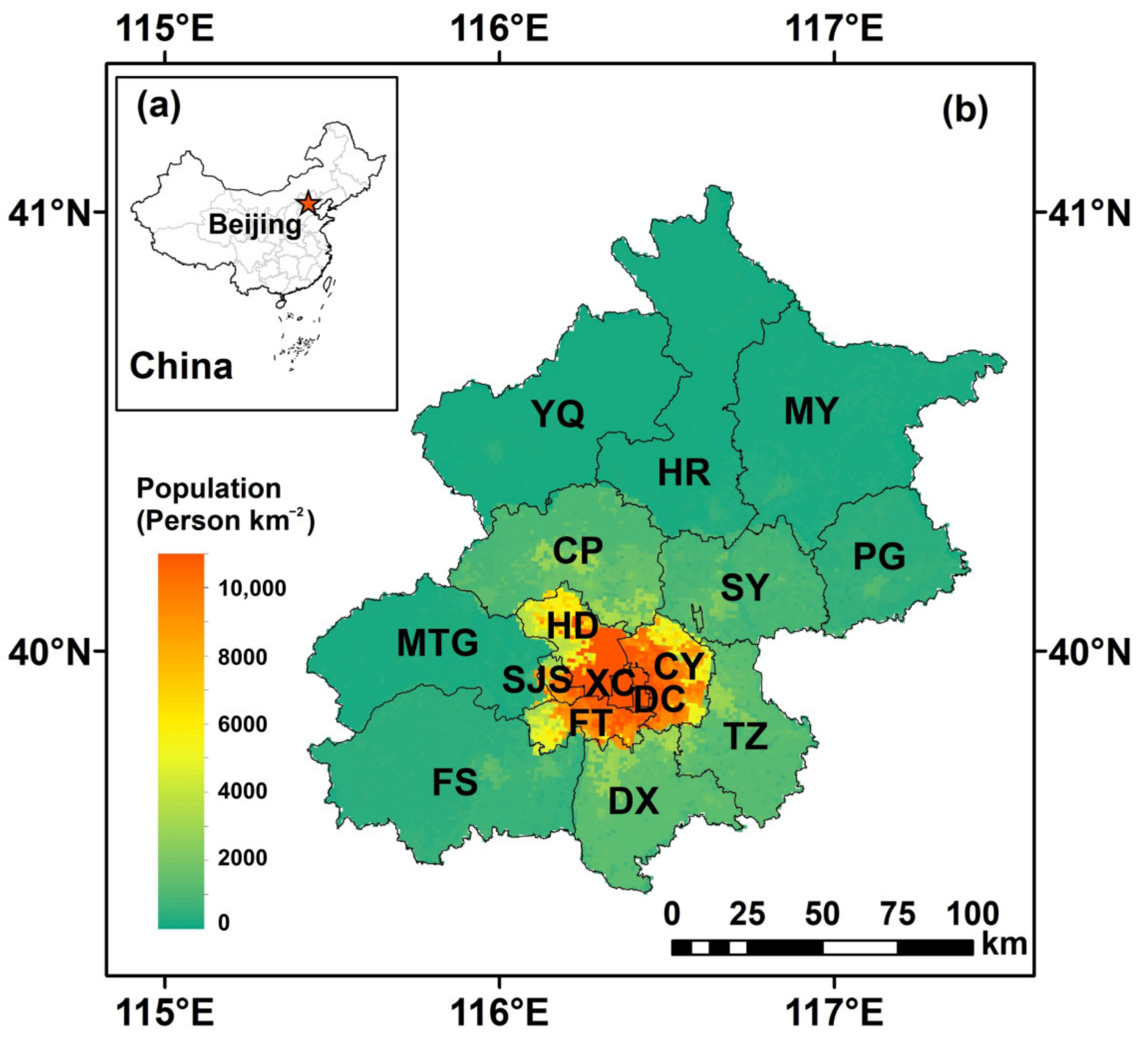
2. Study Area
3. Dataset and Methodology
3.1. Dataset
3.1.1. House Prices
3.1.2. PM2.5 Concentrations
3.1.3. Control Variables
3.1.4. Other Variables
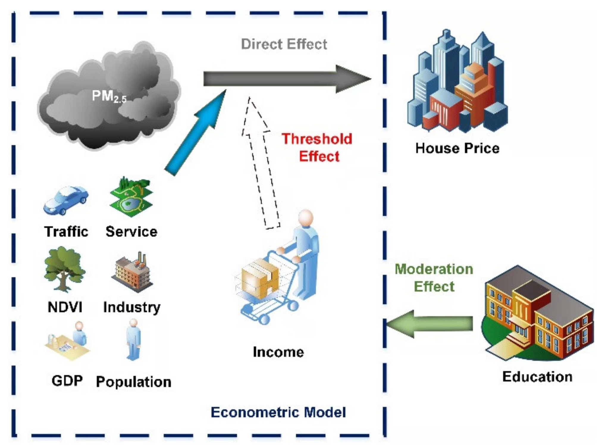
3.2. Methodology
3.2.1. Benchmark Regression Model
3.2.2. Moderating Effect Models
3.2.3. Threshold Effect
3.2.4. Temporal Trend and Correlation Analysis
4. Results and Discussion
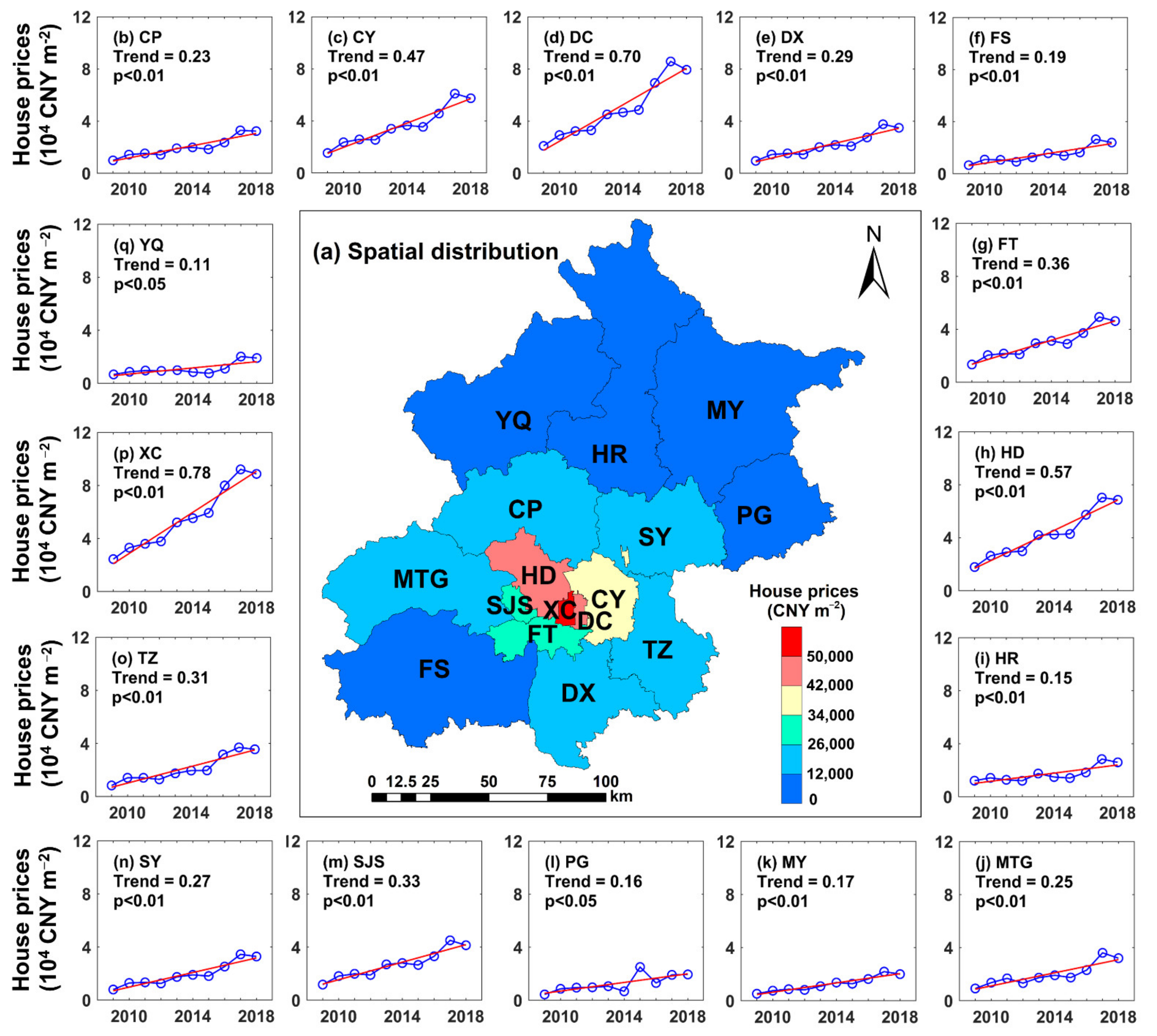
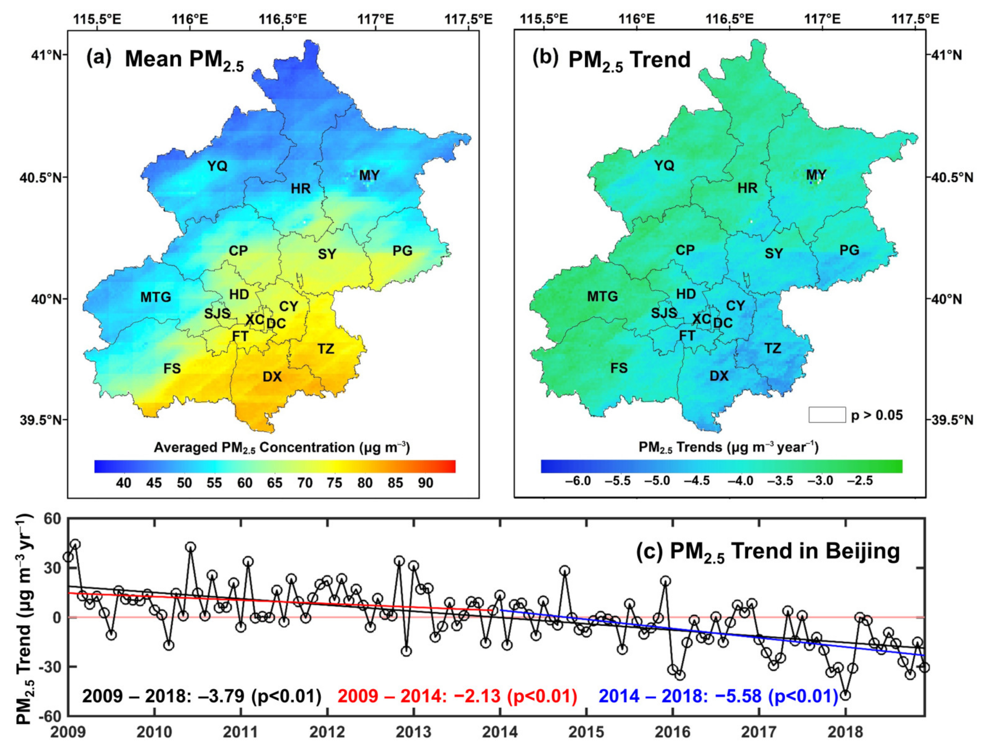
4.1. Spatiotemporal Characteristics of PM2.5 and House Prices
4.2. Spatial Correlation
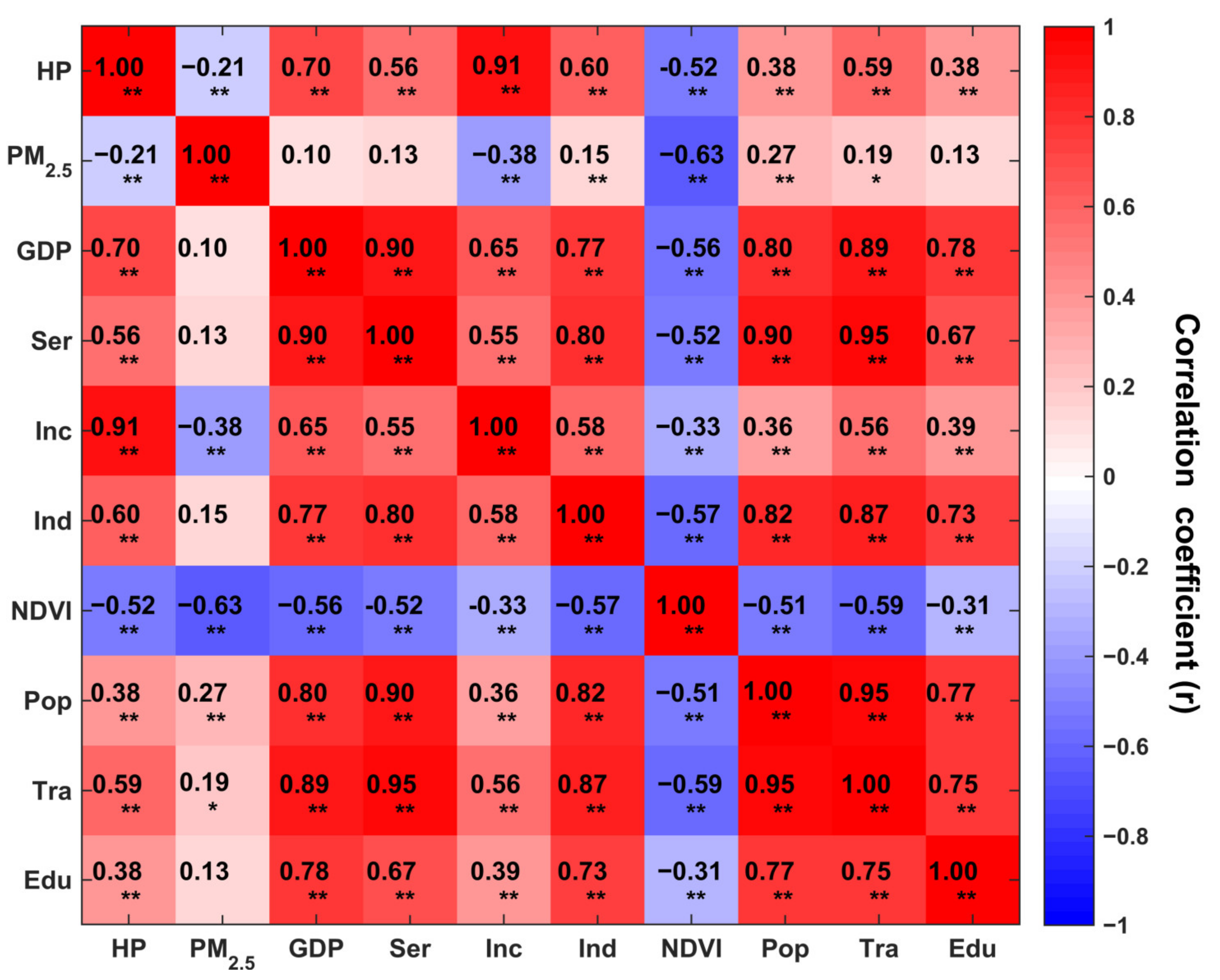
4.3. Correlation Analysis
4.4. Impact of PM2.5 on House Prices
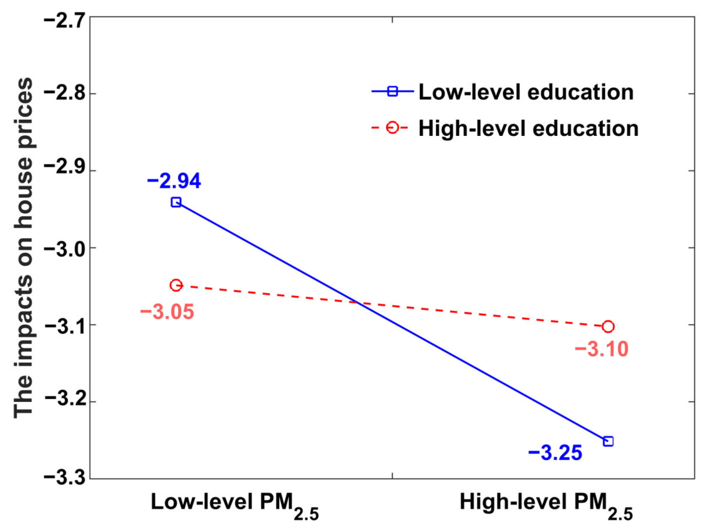
4.5. Moderating Effect of Education
4.6. Threshold Regression Result
4.7. Robustness Test
4.7.1. Endogeneity Problems
4.7.2. Winsorized Robust Measures
5. Conclusions
6. Policy Suggestions
Author Contributions
Funding
Institutional Review Board Statement
Informed Consent Statement
Conflicts of Interest
References
- Geng, G.; Zheng, Y.; Zhang, Q.; Xue, T.; Zhao, H.; Tong, D.; Zheng, B.; Li, M.; Liu, F.; Hong, C.; et al. Drivers of PM2.5 air pollution deaths in China 2002–2017. Nat. Geosci. 2021, 14, 645–650. [Google Scholar] [CrossRef]
- Wei, J.; Li, Z.; Lyapustin, A.; Sun, L.; Peng, Y.; Xue, W.; Su, T.; Cribb, M. Reconstructing 1-km-resolution high-quality PM2.5 data records from 2000 to 2018 in China: Spatiotemporal variations and policy implications. Remote Sens. Environ. 2020, 252, 112136. [Google Scholar] [CrossRef]
- Wei, J.; Li, Z.; Li, K.; Dickerson, R.; Pinker, R.; Wang, J.; Liu, X.; Sun, L.; Xue, W.; Cribb, M. Full-coverage mapping and spatiotemporal variations of ground-level ozone (O3) pollution from 2013 to 2020 across China. Remote Sens. Environ. 2022, 270, 112775. [Google Scholar] [CrossRef]
- Cohen, A.J.; Brauer, M.; Burnett, R.; Anderson, H.R.; Frostad, J.; Estep, K.; Balakrishnan, K.; Brunekreef, B.; Dandona, L.; Dandona, R.; et al. Estimates and 25-year trends of the global burden of disease attributable to ambient air pollution: An analysis of data from the Global Burden of Diseases Study 2015. Lancet 2017, 389, 1907–1918. [Google Scholar] [CrossRef]
- Wei, J.; Liu, S.; Li, Z.; Liu, C.; Qin, K.; Liu, X.; Pinker, R.; Dickerson, R.; Lin, J.; Boersma, K.; et al. Ground-level NO2 surveillance from space across China for high resolution using interpretable spatiotemporally weighted artificial intelligence. Environ. Sci. Technol. 2022. [Google Scholar] [CrossRef]
- Miao, W.; Huang, X.; Song, Y. An economic assessment of the health effects and crop yield losses caused by air pollution in mainland China. J. Environ. Sci. 2017, 56, 102–113. [Google Scholar] [CrossRef] [PubMed]
- Peng, C.; Li, B.; Nan, B. An analysis framework for the ecological security of urban agglomeration: A case study of the Beijing-Tianjin-Hebei urban agglomeration. J. Clean. Prod. 2021, 315, 128111. [Google Scholar] [CrossRef]
- Xue, W.; Zhang, J.; Ji, D.; Che, Y.; Lu, T.; Deng, X.; Li, X.; Tian, Y.; Wei, J. Aerosol-induced direct radiative forcing effects on terrestrial ecosystem carbon fluxes over China. Environ. Res. 2021, 200, 111464. [Google Scholar] [CrossRef]
- Dai, J.; Lv, P.; Ma, Z.; Bi, J.; Wen, T. Environmental risk and housing price: An empirical study of Nanjing, China. J. Clean. Prod. 2019, 252, 119828. [Google Scholar] [CrossRef]
- Jiao, L.; Liu, Y. Geographic Field Model based hedonic valuation of urban open spaces in Wuhan, China. Landsc. Urban Plan. 2010, 98, 47–55. [Google Scholar] [CrossRef]
- Gao, M.; Guttikunda, S.K.; Carmichael, G.R.; Wang, Y.; Liu, Z.; Stanier, C.O.; Saide, P.E.; Yu, M. Health impacts and economic losses assessment of the 2013 severe haze event in Beijing area. Sci. Total Environ. 2015, 511, 553–561. [Google Scholar] [CrossRef] [PubMed]
- Yang, Y.; Luo, L.; Song, C.; Yin, H.; Yang, J. Spatiotemporal Assessment of PM2.5-Related Economic Losses from Health Impacts during 2014–2016 in China. Int. J. Environ. Res. Public Health 2018, 15, 1278. [Google Scholar] [CrossRef] [PubMed]
- Chen, S.; Jin, H. Pricing for the clean air: Evidence from Chinese housing market. J. Clean. Prod. 2018, 206, 297–306. [Google Scholar] [CrossRef]
- Zhang, L.; Yi, Y. What contributes to the rising house prices in Beijing? A decomposition approach. J. Hous. Econ. 2018, 41, 72–84. [Google Scholar] [CrossRef]
- Huang, M.; Lu, B. Measuring the Housing Market Demand Elasticity in China—Based on the Rational Price Expectation and the Provincial Panel Data. Open J. Soc. Sci. 2016, 4, 21–25. [Google Scholar] [CrossRef][Green Version]
- Hui, E.C.-M.; Wang, X.-R.; Jia, S.-H. Fertility rate, inter-generation wealth transfer and housing price in China: A theoretical and empirical study based on the overlapping generation model. Habitat Int. 2016, 53, 369–378. [Google Scholar] [CrossRef]
- Shen, Y.; Liu, H. Housing prices and economic fundamentals: A cross city analysis of china for 1995–2002. Econ. Res. J. 2004, 6, 78–86. [Google Scholar]
- Du, H.; Ma, Y.; An, Y. The impact of land policy on the relation between housing and land prices: Evidence from China. Q. Rev. Econ. Financ. 2011, 51, 19–27. [Google Scholar] [CrossRef]
- Wang, Y.; Wang, S.; Li, G.; Zhang, H.; Jin, L.; Su, Y.; Wu, K. Identifying the determinants of housing prices in China using spatial regression and the ge-ographical detector technique. Appl. Geogr. 2017, 79, 26–36. [Google Scholar] [CrossRef]
- Liu, M.; Ma, Q.-P. Determinants of house prices in China: A panel-corrected regression approach. Ann. Reg. Sci. 2021, 67, 47–72. [Google Scholar] [CrossRef]
- Zhang, Y.; Hua, X.; Zhao, L. Exploring determinants of housing prices: A case study of Chinese experience in 1999–2010. Econ. Model. 2012, 29, 2349–2361. [Google Scholar] [CrossRef]
- Feng, H.; Lu, M. School quality and housing prices: Empirical evidence based on a natural experiment in shanghai, china. J. Hous. Econ. 2013, 22, 291–307. [Google Scholar] [CrossRef]
- Li, H.; Wei, Y.D.; Wu, Y.; Tian, G. Analyzing housing prices in shanghai with open data: Amenity, accessibility and urban structure. Cities 2019, 91, 165–179. [Google Scholar] [CrossRef]
- Ouyang, Y.; Cai, H.; Yu, X.; Li, Z. Capitalization of social infrastructure into China’s urban and rural housing values: Empirical evidence from Bayesian Model Averaging. Econ. Model. 2022, 107, 105706. [Google Scholar] [CrossRef]
- Yu, H. China’s house price: Affected by economic fundamentals or real estate policy? Front. Econ. China 2010, 5, 25–51. [Google Scholar] [CrossRef]
- Xue, W.; Zhang, J.; Zhong, C.; Ji, D.; Huang, W. Satellite-derived spatiotemporal pm2.5 concentrations and variations from 2006 to 2017 in china. Sci. Total Environ. 2020, 712, 134577. [Google Scholar] [CrossRef]
- Ossokina, I.V.; Verweij, G. Urban traffic externalities: Quasi-experimental evidence from housing prices. Reg. Sci. Urban Econ. 2015, 55, 1–13. [Google Scholar] [CrossRef]
- Tsui, W.H.K.; Tan, D.T.W.; Shi, S. Impacts of airport traffic volumes on house prices of New Zealand’s major regions: A panel data approach. Urban Stud. 2017, 54, 2800–2817. [Google Scholar] [CrossRef]
- Le Boennec, R.; Salladarre, F. The impact of air pollution and noise on the real estate market. The case of the 2013 European green capital: Nantes, France. Ecol. Econ. 2017, 138, 82–89. [Google Scholar] [CrossRef]
- Hao, Y.; Zheng, S. Would environmental pollution affect home prices? An empirical study based on china’s key cities. Environ. Sci. Pollut. Res. 2014, 24, 24545–24561. [Google Scholar] [CrossRef]
- Chen, D.; Chen, S. Particulate air pollution and real estate valuation: Evidence from 286 Chinese prefecture-level cities over 2004–2013. Energy Policy 2017, 109, 884–897. [Google Scholar] [CrossRef]
- Sun, B.; Yang, S. Asymmetric and Spatial Non-Stationary Effects of Particulate Air Pollution on Urban Housing Prices in Chinese Cities. Int. J. Environ. Res. Public Health 2020, 17, 7443. [Google Scholar] [CrossRef] [PubMed]
- Zheng, S.; Cao, J.; Kahn, M.E.; Sun, C. Real Estate Valuation and Cross-Boundary Air Pollution Externalities: Evidence from Chinese Cities. J. Real. Estate Financ. Econ. 2013, 48, 398–414. [Google Scholar] [CrossRef]
- Megan, T. China’s three-child policy. Lancet 2021, 397, 2238. [Google Scholar]
- Xue, W.; Zhang, J.; Zhong, C.; Li, X.; Wei, J. Spatiotemporal PM2.5 variations and its response to the industrial structure from 2000 to 2018 in the Beijing-Tianjin-Hebei region. J. Clean. Prod. 2020, 279, 123742. [Google Scholar] [CrossRef]
- Nachtsheim, C.; Neter, J.; Kutner, M.; Wasserman, W. Applied Linear Statistical Models, 5th ed.; McGraw-Hill: New York, NY, USA, 2005. [Google Scholar]
- Hersbach, H.; Bell, B.; Berrisford, P.; Hirahara, S.; Horányi, A.; Muñoz-Sabater, J.; Nicolas, J.; Peubey, C.; Abdalla, S.; Abellan, X.; et al. The era5 global reanalysis. Q. J. R. Meteorol. Society. 2020, 146, 1999–2049. [Google Scholar] [CrossRef]
- David, C. Estimating the return to schooling: Progress on some persistent econometric problems. Econometrica 2001, 69, 1127–1160. [Google Scholar]
- Frankel, J.A.; Romer, D. Does trade cause growth? Am. Econ. Rev. 1999, 89, 379–399. [Google Scholar] [CrossRef]
- Jakob, M.; Haller, M.; Marschinski, R. Will history repeat itself? Economic convergence and convergence in energy use patterns. Energy Econ. 2012, 34, 95–104. [Google Scholar] [CrossRef]
- Jeffrey, M.; Wooldridge. Cluster-sample methods in applied econometrics. Am. Econ. Rev. 2003, 93, 133–138. [Google Scholar]
- Newey, W.; West, K. Autocovariance lag selection in covariance matrix estimation. Rev. Econ. Stud. 1994, 61, 613–653. [Google Scholar] [CrossRef]
- Schultz, T.P. Wage Gains Associated with Height as a Form of Health Human Capital. Am. Econ. Rev. 2002, 92, 349–353. [Google Scholar] [CrossRef]
- Lechene, V.; Pendakur, K.; Wolf, A. Ordinary Least Squares Estimation of the Intrahousehold Distribution of Expenditure. J. Political Econ. 2022, 130, 681–731. [Google Scholar] [CrossRef]
- York, R.; Gossard, M.H. Cross-national meat and fish consumption: Exploring the effects of modernization and ecological context. Ecol. Econ. 2004, 48, 293–302. [Google Scholar] [CrossRef]
- Horrace, W.C.; Oaxaca, R.L. Results on the bias and inconsistency of ordinary least squares for the linear probability model. Econ. Lett. 2006, 90, 321–327. [Google Scholar] [CrossRef]
- Kelejian, H.H.; Prucha, I.R. A Generalized Spatial Two-Stage Least Squares Procedure for Estimating a Spatial Autoregressive Model with Autoregressive Disturbances. J. Real Estate Financ. Econ. 1998, 17, 99–121. [Google Scholar] [CrossRef]
- Wei, J.; Peng, Y.; Mahmood, R.; Sun, L.; Guo, J. Intercomparison in spatial distributions and temporal trends derived from multi-source satellite aerosol products. Atmos. Chem. Phys. 2019, 19, 7183–7207. [Google Scholar] [CrossRef]
- Cai, S.; Wang, Y.; Zhao, B.; Wang, S.; Xing, C.; Hao, J. The impact of the “air pollution prevention and control action plan” on PM2.5 concentrations in jing-jin-ji region during 2012–2020. Sci. Total Environ. 2017, 580, 197–209. [Google Scholar] [CrossRef]
- Xu, T. The Relationship between Interest Rates, Income, GDP Growth and House Prices. Res. Econ. Manag. 2016, 2, 30. [Google Scholar] [CrossRef]
- Efron, B.; Tibshirani, R. Bootstrap methods for standard errors, confidence intervals, and other measures of statistical accuracy. Stat. Sci. 1986, 1, 54–75. [Google Scholar] [CrossRef]


| Abbreviation | Control Variable | Unit | Mean | Std |
|---|---|---|---|---|
| PM2.5 | Annual averaged concentration of PM2.5 | μg m−3 | 67.33 | 15.95 |
| GDP | Gross domestic product | Billion yuan | 98.07 | 118.00 |
| Service | Gross output value of residential services and other services | Million yuan | 71,202.03 | 78,697.96 |
| Income | Per capita disposable income | Yuan | 32,551.19 | 9659.59 |
| Industry | Gross output value of the construction industry | Million yuan | 379.56 | 368.15 |
| NDVI | Normalized Difference Vegetation Index | - | 0.39 | 0.09 |
| Population | Registered population | Thousand person | 920.60 | 572.60 |
| Traffic | Number of private cars | Set | 254,223.80 | 226,015.90 |
| Year | 2009 | 2010 | 2011 | 2012 | 2013 |
| PM2.5 | 0.108 *** | 0.081 *** | 0.102 *** | 0.105 *** | 0.130 *** |
| HP | 0.175 *** | 0.206 *** | 0.216*** | 0.208 *** | 0.205 *** |
| Year | 2014 | 2015 | 2016 | 2017 | 2018 |
| PM2.5 | 0.101 *** | 0.068 *** | 0.108 *** | 0.137 *** | 0.138 *** |
| HP | 0.211 *** | 0.187 *** | 0.203 *** | 0.214 *** | 0.211 *** |
| (1) | (2) | (3) | |
|---|---|---|---|
| OLS Model | Moderating Effect | Threshold Regression | |
| Variables | House Prices | House Prices | House Prices |
| PM2.5 | −0.541 *** | −0.349 ** | |
| (−3.20) | (−2.14) | ||
| GDP | 0.128 *** | 0.157 *** | 1.140 *** |
| (2.66) | (3.04) | (4.73) | |
| Service | 0.093 | 0.060 | 0.235 ** |
| (1.60) | (1.02) | (1.99) | |
| Income | 1.020 *** | 1.085 *** | |
| (8.10) | (8.63) | ||
| Industry | 0.101 ** | 0.110 *** | 0.180 ** |
| (2.53) | (2.70) | (2.51) | |
| NDVI | −0.879 *** | −0.784 *** | −1.041 *** |
| (−6.51) | (−5.61) | (−2.62) | |
| Population | −0.212 *** | −0.283 *** | −0.090 |
| (−4.14) | (−4.97) | (−1.42) | |
| Traffic | −0.036 | −0.009 | 0.228 |
| (−0.62) | (−0.13) | (1.46) | |
| Education | 0.005 | ||
| (0.12) | |||
| Education × PM2.5 | 0.243 *** | ||
| (3.00) | |||
| PM2.5 (Income < θ) | −0.425 * | ||
| (−1.93) | |||
| PM2.5 (Income ≥ θ) | −0.461 ** | ||
| (−2.08) | |||
| Constant | −1.423 | −3.086 * | −12.622 *** |
| (−0.83) | (−1.83) | (−3.11) | |
| Observations | 160 | 160 | 160 |
| R-squared | 0.901 | 0.906 | 0.897 |
| F | p | RSS | MSE | Ctrit10 | Ctrit5 | Ctrit1 | |
|---|---|---|---|---|---|---|---|
| Single (θ = 101,185) | 14.430 | 0.017 | 2.673 | 0.018 | 9.368 | 11.123 | 14.909 |
| (1) | (2) | (3) | |
|---|---|---|---|
| Stage1 | Stage2 | Robust | |
| Variables | House Prices | House Prices | House Prices |
| PM2.5 | −0.897 ** | −0.513 *** | |
| (−2.20) | (−3.06) | ||
| GDP | 0.183 *** | 0.093 * | 0.133 *** |
| (4.06) | (1.71) | (2.82) | |
| Service | 0.027 | 0.119 * | 0.085 |
| (0.45) | (1.89) | (1.51) | |
| Income | 1.314 *** | 0.828 *** | 1.040 *** |
| (13.13) | (3.38) | (8.31) | |
| Industry | 0.091 * | 0.131 ** | 0.099 ** |
| (1.95) | (2.34) | (2.49) | |
| NDVI | −0.674 *** | −1.079 *** | −0.866 *** |
| (−6.46) | (−4.38) | (−6.21) | |
| Population | −0.331 *** | −0.152 ** | −0.200 *** |
| (−6.32) | (−2.10) | (−3.84) | |
| Traffic | 0.053 | −0.066 | −0.047 |
| (0.86) | (−0.92) | (−0.82) | |
| Temperature | −14.255 ** | ||
| (−2.10) | |||
| Constant | 73.330 * | 2.058 | −1.632 |
| (1.92) | (0.50) | (−0.95) | |
| Observations | 160 | 160 | 160 |
| Cragg-Donald Wald F statistics | 43.320 | - | - |
| R-squared | 0.898 | 0.897 | 0.904 |
Publisher’s Note: MDPI stays neutral with regard to jurisdictional claims in published maps and institutional affiliations. |
© 2022 by the authors. Licensee MDPI, Basel, Switzerland. This article is an open access article distributed under the terms and conditions of the Creative Commons Attribution (CC BY) license (https://creativecommons.org/licenses/by/4.0/).
Share and Cite
Xue, W.; Li, X.; Yang, Z.; Wei, J. Are House Prices Affected by PM2.5 Pollution? Evidence from Beijing, China. Int. J. Environ. Res. Public Health 2022, 19, 8461. https://doi.org/10.3390/ijerph19148461
Xue W, Li X, Yang Z, Wei J. Are House Prices Affected by PM2.5 Pollution? Evidence from Beijing, China. International Journal of Environmental Research and Public Health. 2022; 19(14):8461. https://doi.org/10.3390/ijerph19148461
Chicago/Turabian StyleXue, Wenhao, Xinyao Li, Zhe Yang, and Jing Wei. 2022. "Are House Prices Affected by PM2.5 Pollution? Evidence from Beijing, China" International Journal of Environmental Research and Public Health 19, no. 14: 8461. https://doi.org/10.3390/ijerph19148461
APA StyleXue, W., Li, X., Yang, Z., & Wei, J. (2022). Are House Prices Affected by PM2.5 Pollution? Evidence from Beijing, China. International Journal of Environmental Research and Public Health, 19(14), 8461. https://doi.org/10.3390/ijerph19148461