Abstract
The aim of this study is to ascertain the most suitable model for predicting complex odors using odor substance data that has a small number of data and a large number of missing data. First, we compared the data removal and imputation methods, and the method of imputing missing data was found to be more effective. Then, in order to recommend a suitable model, we created a total of 126 models (missing imputation: single imputation, multiple imputations, K-nearest neighbor imputation; data preprocessing: standardization, principal component analysis, partial least square; and predictive method: multiple regression, machine learning, deep learning) and compared them using R2 and mean absolute error (MAE) values. Finally, we investigated variable importance using the best prediction model. The results identified the best model as a combination of multivariate imputation using Bayesian ridge as the missing imputation method, standardization for data preprocessing, and an extremely randomized tree as the predictive method. Among the odor compounds, Methyl mercaptan, acetic acid, and dimethyl sulfide were identified as the most important odor compounds in predicting complex odors.
1. Introduction
Odors from livestock facilities adversely affect both the quality of life of areas neighboring the facility and the working environment of livestock workers. Odors considerably impair quality of life, and the odor substances can cause severe diseases, such as headaches, vomiting, stress and even cancer [1,2,3]. Therefore, it is necessary to improve the environment of livestock facilities by predicting and preventing the occurrence of odors in advance. Currently, Korea’s Malodor Prevention Act enforces concentration regulation on complex odors measured using the olfactory measurement method and concentration evaluations of 17 designated odor substance methods, which are instrumental analysis methods.
The olfactory measurement method has the advantage of being able to respond to various odor substances and evaluate odors in a situation similar to the sense of damage felt by residents of odor-affected areas. However, it cannot guarantee complete objectivity due to differences in individual physiology and olfactory responses affecting the perception of a smell’s concentration [4].
On the other hand, while the odor substance concentration evaluation method presents objective data for a single odor substance, it is insufficient to identify the odor with these substances alone [5]. Therefore, research on odor estimation by measuring the concentration of odor substances is being undertaken in a variety of fields to improve the objectivity of odor evaluation.
Rincón et al. (2019) [6] conducted a study on estimating odor concentration using a statistical method called partial least squares regression (PLSR) by converting the concentration of odor substances from composting plants into Odor Activity Values (OAV).
Man et al. (2020) [7] reported that the estimation performance was excellent during their study to estimate the concentration of odor substances using on-site odor concentration evaluation and laboratory evaluations of odor samples. Similarly, Jonassen et al. (2016) [8] used principal component analysis (PCA) to analyze odor and develop a multivariate statistical prediction method. The study utilized a human panelist and chemical measurements of odorants by Proton-Transfer-Reaction Mass Spectrometry (PTR-MS) on-site measurements of odor concentration measured by dilution to the threshold.
Bylinski et al. (2019) [9] applied artificial neural networks (ANN) and decision trees to predict the odor properties of post-fermentation sludge from two biological-mechanical treatment plants located in the north of Poland. In addition, Luchun Yan et al. (2020) [10] predicted odor intensity by using odor pollutants and a support vector machine (SVM) to perform visual analysis. E. Vigneau et al. (2018) [11] used random forest and PLSR to predict and correlate the characteristics of chemical volatile organic compounds (VOCs) and wine. Similarly, Kang et al. (2020) [12] predicted odor using water quality data and ANN. Hidayat et al. (2021) [13] made the electronic Nose (e-Nose) system to classify the odors in polluted air near a cattle ranch as low, high, or normal. Thus, while many studies based on a large amount of data or complete data are present, studies that utilize a small amount of data or incomplete data are insufficient.
This study was conducted based on a small sample of data (n = 57) with a large amount of missing data. The goal was to use various methods to identify the best model for odor prediction in the case of small odor substances with a large amount of missing data. In this analysis process, missing preprocessing was an essential process since missing this step can adversely affect the outcome. Generally, the removal method is suggested for variables with a high missing rate, it leads to data information loss and can reduce predictive performance [14,15,16]. Hence, we compared the imputation and removal methods for missing data. Finally, we tried to identify the odor substances that have the most influence on odor prediction.
To predict complex odors, data on 15 types of odor substances collected from 10 pig farms were transported to the laboratory for this study. Imputation methods for missing data, such as single imputation, multiple imputations, and K-nearest neighbor (KNN) imputation, were used to figure out the optimal method; and data preprocessing methods, such as standardization, PCA, and PLS, were used to improve prediction performance and speed. Finally, we used multiple regression, machine learning (support vector machine, random forest, extreme randomized tree, XGBoost), and deep learning with three hidden layers as the predictive methods.
This paper presents a description of the data and methods used in Section 2, and in Section 3, the results of the best model method selected based on R2 and mean absolute error (MAE), the results of each part of the prediction process (missing imputation, data preprocessing, predictive method), and variable importance in predicting complex odors are explored over five parts. In Section 4, the limitations of this study and future study topics are discussed and the results of this study are summarized in general.
2. Materials and Methods
2.1. Material
2.1.1. Study Area
Odor compounds were collected from the inside of the finishing pig barns from 10 pig farms of various sizes in Korea. From April to November 2018, data on odors inside 57 pig barns was collected. The stocking density of the pig under investigation was 0.75–1.1 heads/m2. Forced ventilation was present at seven pig farms, and three pig farms had a combination of winch-curtain and forced ventilation. The floor types of pig houses are as follows: five places with partial slat (slat ratio varies from 25% to 70%, respectively), one place with full slat, and two places with manure scraper system.
2.1.2. Data Sampling
Odors in pig houses are caused by incomplete digestion of nutrients in feed and anaerobic fermentation from long-term storage of livestock manure [17,18]. Therefore, evaluation of odor using a single substance is not appropriate, as the odors in the pig houses are generated by a mixed gas in which multiple substances exist in combination [19]. Therefore, in this study, complex odors and 15 species of odor.
The measured odor compounds were Ammonia (NH3), Hydrogen Sulfide (H2S), methyl mercaptan (MM), Dimethyl sulfide (DMS), Dimethyl disulfide (DMDS), Acetic acid (ACA), Propionic acid (PPA), Butyric acid (BTA), Iso-Butyric acid (IBA), Valeric acid (VLA), Iso-Valeric aic (IVA), Phenol (Ph), para-Cresol (p-C), Indole (ID), and Skatole (SK).
When dealing with high concentrations of ammonia, attention should be paid to the sampling rate of ammonia. For ammonia sampling, we used two series-connected impingers. Although Korea’s standard methods for odor examination require sampling at the flow rate of the pump at 10 L/min and a sampling time of 5 min, there is a risk of breakthrough. Therefore, the ammonia sample was collected by passing the sample through the absorbent solution (5 g of boric acid, 50 mL of boric acid solution prepared with 1 L of distilled water) using two series-connected impingers at a rate of 5 L/min for 10 min. Complex odor and sulfur compounds were sampled using the aluminum Tedlar bag.
The complex odor was calculated according to the air dilution olfactory method of Korea’s standard methods for the examination of odor samples and was analyzed within 48 h, five panelists participated and the ammonia was measured using an ultraviolet-visible light spectrophotometer (UV-2700, Shimadzu, Kyoto, Japan) at a wavelength of 640 nm. Meanwhile, sulfur compounds were analyzed using a GC with a pulsed-flame photometric detector (PFPD) (456-GC, Scion instruments, Goes, The Netherlands) equipped with a CP-Sil 5CB column and thermal desorption (TD, Unity + air server, Markes, Bridgend, UK) system with a cold trap. The oven temperature was maintained at 60 °C for 3 min, increased to 160 °C at 8 °C/min, and then maintained at 160 °C for 9 min. All samples were taken at least in triplicate, and every experiment was repeated three times at each condition [20].
The volatile organic compounds (VOCs), VFAs, phenols, and indoles were sampled at 0.1 L/min for 5 min using the 3-bed tube (Carbopack C:Carbopack B:Carbopack X, 1:1:1). The analysis system utilized a system in which thermal desorption (TD) and GC/MSD are connection systems. The TD (unity + air server, Markes, Bridgend, UK) cold trap condition increases a low temp of 5 °C to a high temp of 300 °C, the split flow was 10:1, and the flow path temperature was maintained at 150 °C. VOCs, VFAs, phenols, and indoles were analyzed using a GC (6890N/5973N, Agilent, Santa Clara, CA, USA) equipped with a CP-Wax52CB column (60 m × 0.25 mm × 0.25 um) and an MSD. The oven temperature was initially 45 °C for 5 min, increasing to 250 °C at 5 °C/min, which was then held at 250 °C for 4 min. The ion source temperature was maintained at 230 °C [18]. Table 1 summarizes the conditions of the odor substance analysis device.

Table 1.
Summary of various analytical methods.
Table 2 presents a summary of the collected complex odors and odor substances. The types of all variables are float, and 57 were collected for each variable. In addition, missing data occurred in 11 variables out of 15 explanatory variables. “Dimethyl disulfide” (91.2%), “Dimethyl sulfide” (63.2%), “Methyl mercaptan” (54.4%), “Indole” (36.8%), “Skatole” (14%), “Phenol” “(3.5%), “Pro-panoic acid” (1.8%), “Isobutyric acid” (1.8%), “Normality butyric acid” (1.8%), “Normality valeric acid” (1.8%), and “P-Cresol” (1.8%).
Table 2.
Summary of complex odor and odor substances.
Figure 1 shows the distribution of the missing data in the data used in this study. In this figure, the black part means the observed value and the white part means the missing value.
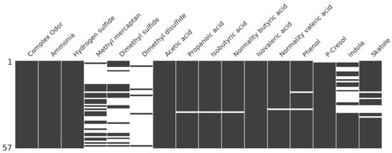
Figure 1.
Map of missing data.
2.2. Methods
In this study, we tried to determine the best prediction model by combining various methods. This study process consisted of missing imputation, data preprocessing, and prediction methods.
The missing data imputation process applied seven statistical methods that are extended to single imputation, multiple imputations, and K-nearest neighbor imputation. The data preprocessing process applied a standardization method that adjust the range of variables equally, and partial least square and principal component analysis methods were used to improve prediction performance and speed [6,8]. Finally, prediction methods applied multiple regression, four types of machine learning (support vector machine, random forest, extreme randomized tree, XGBoost), and deep learning.
These processes created a total of 126 combination models, and the best model was selected with the R2 and MAE [21] obtained by applying the leave-one-out cross-validation (LOOCV) method. Figure 2 shows the workflow of the study and Table 3 describes the notation used in this paper.
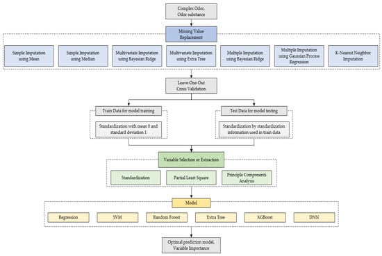
Figure 2.
The overall workflow of the conducted study.
Table 3.
Notation description.
2.2.1. Missing Imputation
We used single imputation (univariate method and multivariate method), multiple imputations, and KNN imputation as a missing imputation method.
- Single imputation
Single imputation is a basic method of imputing missing values, and it is divided into the univariate method, which considers only variables with missing data, and the multivariate method, which considers the relationship with other variables as well. The univariate method imputes missing data with statistical values such as the mean, median, and mode of the corresponding data.
The multivariate method models the imputation variable as y and the other variable as x in order to impute missing data. There are several available methods such as Bayesian ridge [22] and extreme randomized tree [23]. Despite being easy and fast to calculate, there is a chance of inaccuracies, arising from bias or underestimation of the standard error of the estimator affecting the results.
- Multiple imputations
Multiple imputations [24] is a method proposed to compensate for the shortcomings of the single imputation method. This method utilizes multiple single imputations and consists of three steps: imputation, analysis, and pooling.
In the imputation step, m imputation datasets are generated using the single imputation method, and in the analysis step, statistical values (estimator, variance) are calculated from the m imputation datasets created in the previous step. Finally, in the pooling step, the statistical information from the previous step is combined and the missing value is imputed to the optimal value. Figure 3 is an example of the multiple imputation method.
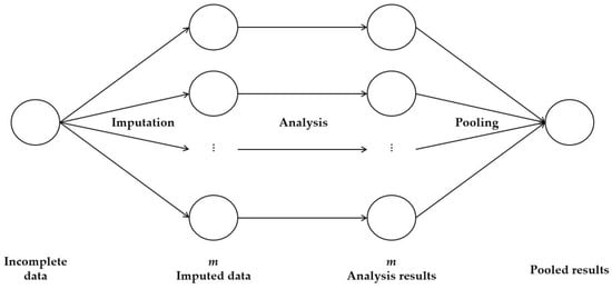
Figure 3.
Example of multiple imputations.
- K-nearest neighbor (KNN) imputation
KNN imputation finds the nearest n neighbor data through the Euclidean distance metric from the missing data to be imputed. It then imputes the missing data using the weighted or unweighted average of the neighbor data. Figure 4 shows KNN imputation with k = 3 [25].
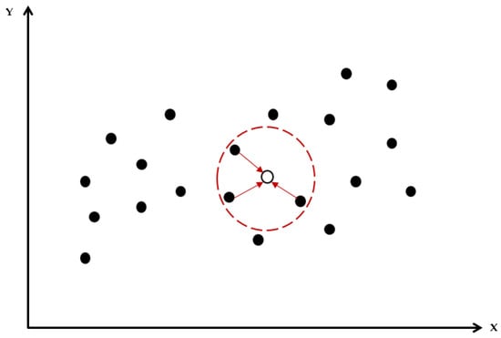
Figure 4.
(k = 3) K-nearest neighbor imputation.
2.2.2. Data Preprocessing
We applied data preprocessing, such as PCA and PLS, to improve prediction performance and speed [6,8].
- PCA
PCA [26] is an unsupervised feature extraction method that projects high-dimensional data with p variables into low-dimensional data with k variables using only explanatory variable information. The principal component (i = 1, 2,⋯, k), which is a new variable generated using PCA, can be generated as many times as the value of p, which is the maximum number of original variables. In general, the number of principal components that explain more than 70–80% of the variance of the original variable is selected and used.
The variable created by PCA has the following three characteristics. (1) the principal component is generated as a linear combination of the original variables; (2) an axis is created and projected in the direction of the greatest dispersion; (3) it is a useful method to solve the problem of multicollinearity because each is independent of each other.
- PLS
PLS [27] is a method that reduces the dimension of variables by creating new variables through linear combinations between variables when there is a problem of multicollinearity between variables in multivariate data with multiple variables. In particular, this is a useful method when the number of variables (p) is greater than the number (n) of data.
Unlike PCA, which uses only explanatory variable information, it is a supervised feature extraction method that also uses response variable information. The latent variable (T), which is a variable extracted through linear combination with PLS, can be created as many times as the value of p, which is the maximum number of original variables. The optimal number of latent variables is selected based on the mean square error (MSE) [21].
2.2.3. Prediction Methods
We used three types of prediction methods—statistical method, machine learning method, deep learning method.
- Multiple linear regression
Multiple linear regression is an extension of simple linear regression. It is a regression used when there are two or more explanatory variables, and is expressed as shown in Equation (1) below.
where are the regression coefficients in the form of constant values, is the unexplained error, and is the i-th observation value of the p-th explanatory variable.
- Support vector machine (SVM)
The basic idea of SVM [28] is to classify data by creating a hyperplane. While it is well distinguished in a linear problem, additional work using the kernel function in high-dimensional problems such as nonlinear problems. The optimal hyperplane is determined in a way that maximizes the margin. That is, the hyperplane with the largest distance from the data is selected. In the case of regression data, the hyperplane is the regression line. Figure 5 shows a support vector machine with two variables.
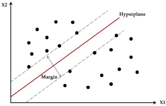
Figure 5.
Support vector machine with two variables.
- Ensemble tree
Ensemble tree is a method of applying ensemble, which is a method of making better generalization performance by connecting multiple classifiers into a single meta-classifier, to a decision tree. Here, the decision tree is an analysis method that charts decision rules in a tree-like structure.
- Random forest
Random forest [29] is a type of ensemble learning method that uses multiple decision trees constructed during the training process to classify or predict datasets. That is, it is an ensemble of decision trees that improves generalization performance and reduces overfitting by averaging several (deep) decision trees to solve the problem of the large variance in individual trees.
Random forests are not as easy to interpret as decision trees, but they generally do not require pruning (a way to simplify the model), necessitating less effort for tuning. Additionally, they have fewer hyperparameters (number of trees, bootstrap size, number of variables to be selected in each split). Figure 6 is an example of the random forest with k decision trees.
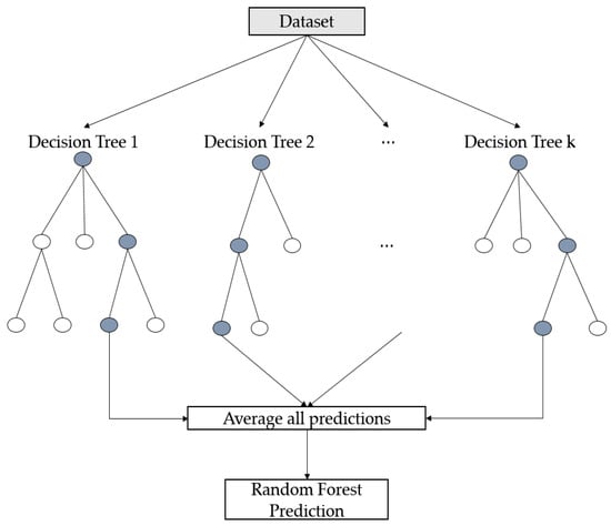
Figure 6.
Example of the random forest with k decision trees.
- 2.
- Extremely randomized tree (Extra Tree)
Extra Tree is a method constructed using the ensemble method of a non-pruned decision tree or regression tree [23]. It is similar to the random forest method, however, while random forest uses sampling without replacement when creating multiple trees based on bootstrap, Extra Tree uses sampling with replacement and uses Whole Original data.
In addition, random forest calculates the information gain for all features in the split process and splits based on this value; however, in the case of Extra Tree, the split is performed by randomly selecting a variable when performing the split process. Therefore, it saves computation time compared to random forest, and reduces bias and variance by performing splits randomly.
- 3.
- XGBoost
XGBoost (extreme gradient boosting) is a modified method of gradient boosting machine (GBM) [30] and is in the form of a tree to which gradient boosting is applied. The biggest advantage of XGBoost is that parallel processing is possible and the amount of computation is reduced. In addition, overfitting can be prevented by shrinkage and column subsampling, Additionally, by using the approximate algorithm, Weighted Quantile Sketch, and Sparsity-aware Split Finding method instead of the Exact Greedy Algorithm for the split operation, the calculation speed is increased, allowing excellent performance results to be obtained even for datasets with many missing values and zeros [31].
- Deep neural network (DNN)
DNN is a learning method based on ANN. That is, it is an ANN with multiple hidden layers. ANN is a method created based on neurons that have the characteristic of transmitting when the size of a stimulus is greater than a specific value among the components of human nerves. DNN consists of a total of three layers connected by weights: input layer, hidden layer, and output layer.
DNN consists of a forward propagation process that calculates output and a back propagation [32] process that updates weights. Forward propagation receives the value of the explanatory variable through each node of the input layer, multiplies it with an appropriate weight, and delivers it to the node of the hidden layer. In the hidden layer, the received values are transformed through linear combination and an appropriate activation function (a function that determines an output value from an input value). It is then multiplied by a weight value and delivered to each node of the output layer.
Each node of the output layer finally outputs the predicted value through a linear combination of the received value and an appropriate activation function. Back propagation is a process of adjusting weights by using mathematical differentiation and chain rule to output an optimal prediction value. Figure 7 is an example of the DNN with n hidden layers of three nodes.
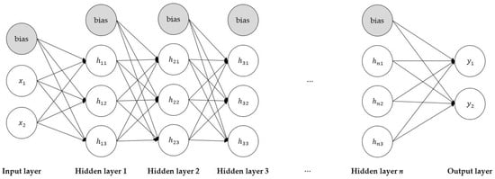
Figure 7.
Example of the DNN with n hidden layers of 3 nodes.
2.2.4. Leave-One-Out Cross-Validation (LOOCV)
Since the data used in this study have a small number of samples, model testing was performed using LOOCV. LOOCV is a type of K-fold cross-validation (CV) [33], that helps to prevent overfitting and underfitting problems. The CV method is a method that randomly divides the training data into k folds, trains the model with k − 1 folds, and evaluates the performance of the model with the remaining one fold.
LOOCV evaluates the performance of a model with only one observation value after training a model with n − 1 data out of n data. In this case, MSE is mainly used for model performance evaluation. LOOCV has a total of n performance evaluation results, and the average of these n performance evaluations is used as a performance evaluation index. Figure 8 is an example of LOOCV for n data.
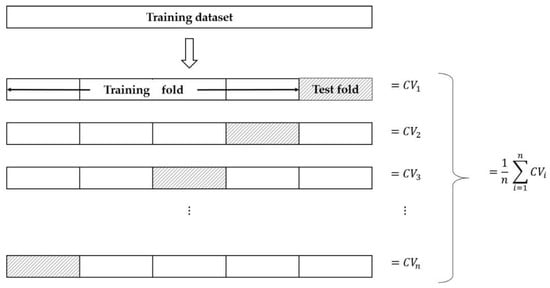
Figure 8.
Example of LOOCV for n data.
3. Results
3.1. Proposed Method
A combination of seven missing imputation methods, three data preprocessing methods, and six predictive methods were used and compared. We adopted R2 as a model selection criterion that applied LOOCV to regression analysis using observed and predicted values. Table 4 shows the top five results selected based on R2 and MAE from a total of 126 model results. In the results, multivariate imputation and KNN imputation were mainly used as imputation methods for missing data, and standardization and PCA were used as data preprocessing methods. Finally, Extra Tree, XGBoost, and random forest are excellent predictive methods. The machine learning method was observed to be superior to multiple regression and deep learning, and among the machine learning methods, the ensemble tree method was found to be the most suitable. The results of the prediction process (missing imputation, data preprocessing, predictive method) are as follows.
Table 4.
Top 5 proposed results based on R2 and MAE when missing data is imputed.
3.2. Missing Imputation
As mentioned above, the data used in the study have a lot missing, and in this case, the removal method is usually used. However, the removal method leads to the loss of information. Therefore, in this study, only the dimethyl disulfide variable with a missing rate of 91.2% was removed and the remaining variables were imputed. The suitability of the imputation method was ensured by comparing it to a model that used the removal method. Table 5 shows the top results of the five models when variables with high missing ratios were removed.
Table 5.
Top 5 proposed results based on R2 and MAE when missing data is not imputed.
A comparison of the results of the imputation and removal models revealed that R2 and MAE were superior in the case of imputing. Therefore, it was ascertained that the imputation method was better than the removal method when there were high levels of missing data.
Figure 9 is a correlation heatmap of the data imputed by multivariate imputation using the Bayesian ridge and KNN imputation used in the upper half of Table 3 among the missing imputation methods. Table 5 shows the correlation results for all the imputation methods used for missing data.
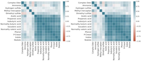
Figure 9.
Heatmap complete data by best imputation method. (left) Heatmap of data using multivariate imputation using Bayesian ridge. (right) Heatmap of data using KNN imputation.
Table 6 shows that hydrogen sulfide and dimethyl sulfide had a negative correlation with the complex odor in all the results, which means that the complex odor decreased as the two substances increased. Since the other 12 odor substances had a positive correlation, it was inferred that the complex odor increased with the value of the variable.
Table 6.
Correlation results by imputation method.
The variable that had the most influence on the complex odor evaluated by the correlation coefficient was methyl mercaptan, followed by p-cresol, acetic acid, ammonia, and indole in that order, and the variable with the least influence was hydrogen sulfide. The results of using data preprocessing to improve prediction performance on imputed data are as follows.
3.3. Data Preprocessing
In this study, data preprocessing was used to improve prediction performance and speed. As a result, the most effective data preprocessing methods used were ascertained to be the standardization and PCA methods. Figure 10 shows a boxplot of the data imputed by multivariate imputation using the Bayesian ridge, the missing imputation method used in the best prediction model, and a boxplot with standardization applied to the data.
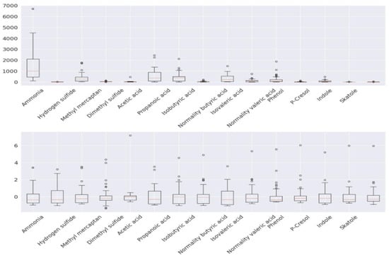
Figure 10.
(top) Boxplot of data imputed by multivariate imputation using Bayesian ridge. (bottom) Boxplot with standardization applied to top data.
The results show that there is a difference in the range of each variable before standardization is applied. As this can hinder the interpretation of the analysis results, standardization was used to match the ranges of each variable. Next, in the PCA method, the number of principal components was selected as a number that could explain 85% of the total variation, and as a result, four components were used.
In Table 3, standardization was used in the best model, but PCA was used in the second and third best models. Therefore, it is sufficient to use only four principal components from the 14 types of odor substances. It is considered that when there is a large number of data samples, using PCA will be useful in terms of cost. Figure 11 shows a plot of PC1 and PC2 among the four principal components. The explanatory power of PC3 (7.5%) and PC4 (7.3%) is rather low, so only PC1 and PC2 are described here.
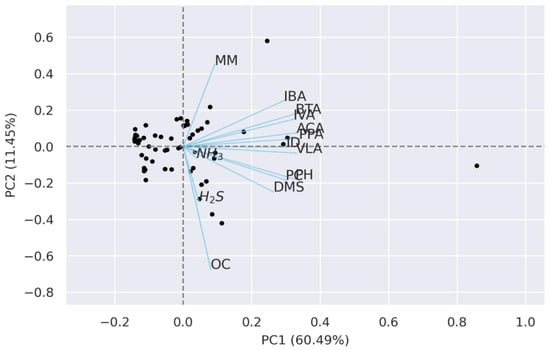
Figure 11.
The loading plot about PC1 and PC2.
In Figure 11, it can be seen that the two principal components account for 71.89% of the total variance (PC1: 60.49%, PC2: 11.45%). While PC1 consists of a positive relationship with all variables, PC2 was found to have a negative relationship with some variables.
Table 7 denotes the loading values of PC1, PC2, PC3, and PC4. PC1 was affected by VOCs variables except for acetic acid, and PC2 showed a positive correlation with the sulfur compound dimethyl sulfide and a negative correlation with ammonia, so it was found to be affected by the fluctuations of these two variables. PC3 showed a strong positive relationship with hydrogen sulfide. Finally, PC4 is confirmed to have a strong positive relationship with the sulfur compound methyl mercaptan and a negative relationship with the VOC acetic acid.
Table 7.
Loading values of principal component analysis.
3.4. Prediction Method Performance
A total of six prediction methods—multiple linear regression, SVM, random forest, Extra Tree, XGBoost, and deep learning were used to predict complex odors with odor substances. Table 4 shows that the most optimal prediction methods were Extra Tree, XGBoost, and random forest. That is, the ensemble tree-based machine learning method is superior to multiple regression or deep learning.
Figure 12 shows the prediction results using the top three models suggested in Table 4 and the results using the average of the predicted values of these three models as the predicted values.
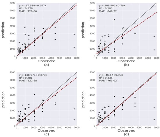
Figure 12.
(a) Prediction result by (multivariate imputation using Bayesian ridge, standardization, Extra Tree, (b) Prediction result by (KNN Imputation, PCA, XGBoost), (c) Prediction result by (KNN Imputation, PCA, random forest), (d) Prediction result by average of the above three results.
In the results of (b) and (c) in Figure 12, the intercepts of the regression lines (dotted red line) for the predicted value and the observed values were positive, which implies that the predicted mean was higher than the observed values for two models.
Additionally, it can be observed from Figure 12 that when the observed values are small, the regression line (dotted red line) is above the solid black line (a straight line with a slope of 1 and an intercept of 0). However, when the observed values increase, the regression line and the black line intersect, suggesting that it is overestimated before the intersection (when the dotted red line is above the solid black line) and underestimated after the intersection (when the dashed red line is below the solid black line).
Whereas, (a) and (d) in Figure 12 show that the intercept of the regression line is negative, implying that, unlike the results of the three models above, the average was predicted lower than the observed values. In addition, the regression line and the black solid line do not intersect and are always located below, indicating an overall underestimation.
As a result of the predicted values, the predicted values of the top model in Table 4 gave the best prediction results than the predicted values using the average (d). The regression line was the closest to the black solid line (a straight line with a slope of 1 and an intercept of 0).
3.5. Variable Importance
In this study, the contribution of odor substances to the prediction of complex odors was investigated. Variable importance [34,35] is a method of identifying the most necessary variable in the creation of a model, and is not based on how much the variable affects the value change of the response variable.
Variable importance uses data not included in the Bootstrap (resampling method without replacement) set used in the ensemble tree-based model training process called “out of bag” (OOB), and is the variable importance of the i-th variable, which is obtained using Equation (2) below. In the equation, is the OOB error of the j-th tree, and is the OOB error of the j-th tree for the dataset in which the values of the i-th variable are randomly mixed.
The variable importance was confirmed using the model of the combination of multivariate imputation using the Bayesian ridge, standardization, and Extra Tree, which revealed the best prediction performance in Table 4. Figure 13 is a plot of the variable importance for predicting complex odors.
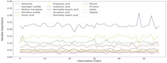
Figure 13.
Variable importance plot about the best model in Table 3.
Since LOOCV was used in this study, Figure 13 is shown as a line-type plot because it had variable importance according to the number of observations (n = 57) for each odor substance. The variable importance value reveals that the most important variable in predicting complex odor is methyl mercaptan, followed by acetic acid, dimethyl sulfide, ammonia, and indole, and the least important variable was isobutyric acid.
Figure 14 shows the variable importance values as a boxplot, with the same results as Figure 13. The least important variable was different from the correlation coefficient result in the missing imputation part of Section 3, but the upper result was similar.
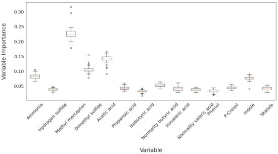
Figure 14.
Boxplot of the variable importance about the best model in Table 3.
4. Discussion and Conclusions
Although odor-related research is conducted in a variety of fields, most studies use large amounts of data or complete data. However, in this study, we tried to use odor substances data that contained variables with a small number of samples (n = 57) and a high rate of missing data to find the most suitable model for odor prediction.
First, we compared the removal method and the imputation method to ascertain the appropriate method for dealing with missing data values. The results showed that the imputation method was more effective than the removal method. Therefore, with these types of data, it is better to consider the imputation method rather than the unconditional removal method for high levels of missing data. Comparing various models for the imputation data, the best model was identified as multivariate imputation using the Bayesian ridge as the missing imputation method, standardization for data preprocessing, and an extremely randomized tree as a predictive method. While the R2 value for prediction was not high, it is expected that better prediction results will be obtained if additional data is secured.
Next, as a result of the variable importance, methyl mercaptan was revealed as the most important variable, followed by acetic acid, dimethyl sulfide, ammonia, and indole as important variables. The least important variable was found to be isobutyric acid. This is very similar to the correlation result between complex odors and odor substances obtained from imputation data. As a result of the correlation, only two variables, hydrogen sulfide and dimethyl sulfide, showed a negative correlation in the complex odor. That is, it was revealed that complex odors decrease with an increase in hydrogen sulfide and dimethyl sulfide values, while it increases with increases in the values of the other 12 odor substances.
This study used laboratory data. However, in real livestock environments, IoT (Internet of Things) sensor devices are used to collect odor substance data. Due to the nature of data collection using sensors, data being missing due to various causes is a frequent problem [36]. Therefore, we consider that it is applicable to the actual livestock environment that we used data with missing values.
Although this study focused on discovering the best prediction model, we expect that it can be extended to various studies in the future. We will compare the results of this study with the results using the workflow of this study on vast data or data without missing information. In addition, we intend to conduct research to improve predictive performance by applying Hyperparameter Optimization to the proposed prediction model. These future studies are expected to develop our workflow and then we will be able to identify more clearly the odor substances and critical points causing the odor using methods such as LIME (local interpretable model-agnostic explanations) and SHAP (shapely additive explanations) [37,38,39]. We expect that these studies will make it easier to manage odor substances.
Therefore, we consider applied studies. For example, odor source prediction [40], odor intensity prediction according to distance, odor intensity classification [13] and application for other types of odors other than livestock odors, such as water [12] and factory [41] odors. These studies will help to significantly positively impact the lives of odor facilities, such as livestock facilities, as well as the lives of the residents in the surrounding area.
Author Contributions
Data curation, D.-H.L.; software, D.-H.L.; investigation S.-E.W.; formal analysis, D.-H.L.; funding acquisition, T.-Y.H., S.-E.W. and M.-W.J.; supervision, T.-Y.H.; writing—original draft, D.-H.L.; writing—review and editing, T.-Y.H., S.-E.W. and M.-W.J. All authors have read and agreed to the published version of the manuscript.
Funding
This research was supported by the Basic Science Research Program through the National Research Foundation of Korea (NRF) funded by the Ministry of Education (2017R1D1A3B03028084, 2019R1I1A3A01057696). This work was supported by the Korean Institute of Planning and Evaluation for Technology in Food, Agriculture and Forestry (IPET) and Korea Smart Farm R&D Foundation (KosFarm) through the Smart Farm Innovation Technology Development Program, funded by the Ministry of Agriculture, Food and Rural Affairs (MAFRA) and the Ministry of Science and ICT (MSIT), Rural Development Administration (RDA) (421020-03).
Institutional Review Board Statement
Not applicable.
Informed Consent Statement
Not applicable.
Data Availability Statement
The datasets generated during and/or analyzed during the current study are available from the corresponding author on reasonable request.
Conflicts of Interest
The authors declare no conflict of interest.
References
- Wojnarowska, M.; Soltysik, M.; Turek, P.; Szakiel, J. Odour nuisance as a consequence of preparation for circular economy. Eur. Res. Stud. J. 2020, 23, 128–142. [Google Scholar] [CrossRef]
- Leníček, J.; Beneš, I.; Rychlíková, E.; Šubrt, D.; Řezníček, O.; Roubal, T.; Pinto, J.P. VOCs and odor episodes near the German–Czech border: Social participation, chemical analyses and health risk assessment. Int. J. Environ. Res. Public Health 2022, 19, 1296. [Google Scholar] [CrossRef] [PubMed]
- Byliński, H.; Gębicki, J.; Namieśnik, J. Evaluation of health hazard due to emission of volatile organic compounds from various processing units of wastewater treatment plant. Int. J. Environ. Res. Public Health 2019, 16, 1712. [Google Scholar] [CrossRef] [PubMed]
- Kim, J.B.; Jeong, S.J. The relationship between odor unit and odorous compounds in control areas using multiple regression analysis. J. Environ. Health Sci. 2009, 35, 191–200. [Google Scholar] [CrossRef]
- Kim, J.B.; Jeong, S.J.; Song, I.S. The concentrations of sulfur compounds and sensation of odor in the residential area around Banwol-Sihwa industrial complex. J. Korean Soc. Atmos. Environ. 2007, 23, 147–157. [Google Scholar] [CrossRef]
- Rincón, C.A.; De Guardia, A.; Couvert, A.; Wolbert, D.; Le Roux, S.; Soutrel, I.; Nunes, G. Odor concentration (OC) prediction based on odor activity values (OAVs) during composting of solid wastes and digestates. Atmos. Environ. 2019, 201, 1–12. [Google Scholar] [CrossRef]
- Man, Z.; Dai, X.; Rong, L.; Kong, X.; Ying, S.; Xin, Y.; Liu, D. Evaluation of storage bags for odour sampling from intensive pig production measured by proton-transfer-reaction mass-spectrometry. Biosyst. Eng. 2020, 189, 48–59. [Google Scholar] [CrossRef]
- Hansen, M.J.; Jonassen, K.E.; Løkke, M.M.; Adamsen, A.P.S.; Feilberg, A. Multivariate prediction of odor from pig production based on in-situ measurement of odorants. Atmos. Environ. 2016, 135, 50–58. [Google Scholar] [CrossRef]
- Byliński, H.; Sobecki, A.; Gębicki, J. The use of artificial neural networks and decision trees to predict the degree of odor nuisance of post-digestion sludge in the sewage treatment plant process. Sustainability 2019, 11, 4407. [Google Scholar] [CrossRef]
- Yan, L.; Wu, C.; Liu, J. Visual analysis of odor interaction based on support vector regression method. Sensors 2020, 20, 1707. [Google Scholar] [CrossRef]
- Vigneau, E.; Courcoux, P.; Symoneaux, R.; Guérin, L.; Villière, A. Random forests: A machine learning methodology to highlight the volatile organic compounds involved in olfactory perception. Food Qual. Prefer. 2018, 68, 135–145. [Google Scholar] [CrossRef]
- Kang, J.H.; Song, J.; Yoo, S.S.; Lee, B.J.; Ji, H.W. Prediction of odor concentration emitted from wastewater treatment plant using an artificial neural network (ANN). Atmosphere 2020, 11, 784. [Google Scholar] [CrossRef]
- Hidayat, R.; Wang, Z.H. Odor classification in cattle ranch based on electronic nose. Int. J. Data Sci. 2021, 2, 104–111. [Google Scholar]
- Graham, J.W. Missing data analysis: Making it work in the real world. Annu. Rev. Psychol. 2009, 60, 549–576. [Google Scholar] [CrossRef]
- Dinh, D.T.; Huynh, V.N.; Sriboonchitta, S. Clustering mixed numerical and categorical data with missing values. Inf. Sci. 2021, 571, 418–442. [Google Scholar] [CrossRef]
- Li, X.; Wu, Z.; Zhao, Z.; Ding, F.; He, D. A mixed data clustering algorithm with noise-filtered distribution centroid and iterative weight adjustment strategy. Inf. Sci. 2021, 577, 697–721. [Google Scholar] [CrossRef]
- Jensen, B.B.; Jørgensen, H. Effect of dietary fiber on microbial activity and microbial gas production in various regions of the gastrointestinal tract of pigs. Appl. Environ. Microbiol. 1994, 60, 1897–1904. [Google Scholar] [CrossRef]
- Jang, Y.N.; Jung, M.W. Biochemical changes and biological origin of key odor compound generations in pig slurry during indoor storage periods: A pyrosequencing approach. BioMed Res. Int. 2018, 2018, 3503658. [Google Scholar] [CrossRef]
- Ministry of Environment (ME). Odor Management Manual; Ministry of Environment (ME): Sejong-si, Korea, 2012.
- Jang, Y.N.; Hwang, O.; Jung, M.W.; Ahn, B.K.; Kim, H.; Jo, G.; Yun, Y.M. Comprehensive analysis of microbial dynamics linked with the reduction of odorous compounds in a full-scale swine manure pit recharge system with recirculation of aerobically treated liquid fertilizer. Sci. Total Environ. 2021, 777, 146122. [Google Scholar] [CrossRef]
- Moriasi, D.N.; Gitau, M.W.; Pai, N.; Daggupati, P. Hydrologic and water quality models: Performance measures and evaluation criteria. Trans. ASABE 2015, 58, 1763–1785. [Google Scholar]
- Burnaev, E.; Vovk, V. Efficiency of conformalized ridge regression. In Proceedings of the Conference on Learning Theory, Barcelona, Spain, 13–15 June 2014; PMLR: USA, 2014; pp. 605–622. [Google Scholar]
- Geurts, P.; Ernst, D.; Wehenkel, L. Extremely randomized trees. Mach. Learn. 2006, 63, 3–42. [Google Scholar] [CrossRef]
- Schafer, J.L. Multiple imputation: A primer. Stat. Methods Med. Res. 1999, 8, 3–15. [Google Scholar] [CrossRef] [PubMed]
- Pan, L.; Li, J. K-nearest neighbor based missing data estimation algorithm in wireless sensor networks. Wirel. Sens. Netw. 2010, 2, 115. [Google Scholar] [CrossRef]
- Abdi, H.; Williams, L.J. Principal component analysis. Wiley Interdiscip. Rev. Comput. Statistics 2010, 2, 433–459. [Google Scholar] [CrossRef]
- Tobias, R.D. An introduction to partial least squares regression. In Proceedings of the Twentieth Annual SAS Users Group International Conference, Orlando, FL, USA, 2–5 April 1995; SAS Institute Inc.: Cary, NC, USA, 1995. [Google Scholar]
- Pradhan, A. Support vector machine-a survey. Int. J. Emerg. Technol. Adv. Eng. 2012, 2, 82–85. [Google Scholar]
- Breiman, L. Random forests. Mach. Learn. 2001, 45, 5–32. [Google Scholar] [CrossRef]
- Friedman, J.H. Greedy function approximation: A gradient boosting machine. Ann. Stat. 2001, 29, 1189–1232. [Google Scholar] [CrossRef]
- Chen, T.; Guestrin, C. Xgboost: A scalable tree boosting system. In Proceedings of the 22nd ACM Sigkdd International Conference on Knowledge Discovery and Data Mining, San Francisco, CA, USA, 13–17 August 2016; pp. 785–794. [Google Scholar]
- Hecht-Nielsen, R. Theory of the backpropagation neural network. In Neural Networks for Perception; Academic Press: Cambridge, MA, USA, 1992; pp. 65–93. [Google Scholar]
- Kohavi, R. A study of cross-validation and bootstrap for accuracy estimation and model selection. In Proceedings of the International Joint Conference on Artificial Intelligence, San Francisco, CA, USA, 20–25 August 1995; pp. 1137–1145. [Google Scholar]
- Strobl, C.; Boulesteix, A.L.; Zeileis, A.; Hothorn, T. Bias in random forest variable importance measures: Illustrations, sources and a solution. BMC Bioinform. 2007, 8, 1–21. [Google Scholar] [CrossRef]
- Wei, P.; Lu, Z.; Song, J. Variable importance analysis: A comprehensive review. Reliab. Eng. Syst. Saf. 2015, 142, 399–432. [Google Scholar] [CrossRef]
- Faizin, R.N.; Riasetiawan, M.; Ashari, A. A Review of Missing Sensor Data Imputation Methods. In Proceedings of the 2019 5th International Conference on Science and Technology (ICST), Yogyakarta, Indonesia, 30–31 July 2019; pp. 1–6. [Google Scholar]
- Heskes, T.; Sijben, E.; Bucur, I.G.; Claassen, T. Causal shapley values: Exploiting causal knowledge to explain individual predictions of complex models. Adv. Neural Inf. Process. Syst. 2020, 33, 4778–4789. [Google Scholar]
- Lundberg, S.M.; Lee, S.I. A unified approach to interpreting model predictions. In Proceedings of the Advances in Neural Information Processing Systems 30, Long Beach, CA, USA, 4–9 December 2017. [Google Scholar]
- Das, A.; Rad, P. Opportunities and challenges in explainable artificial intelligence (xai): A survey. arXiv 2020, arXiv:2006.11371. [Google Scholar]
- Wojnarowska, M.; Ilba, M.; Szakiel, J.; Turek, P.; Sołtysik, M. Identifying the location of odour nuisance emitters using spatial GIS analyses. Chemosphere 2021, 263, 128252. [Google Scholar] [CrossRef] [PubMed]
- Velič, A.; Šurina, I.; Ház, A.; Vossen, F.; Ivanova, I.; Soldán, M. Modeling of Odor from a Particleboard Production Plant. J. Wood Chem. Technol. 2020, 40, 116–125. [Google Scholar] [CrossRef]


Publisher’s Note: MDPI stays neutral with regard to jurisdictional claims in published maps and institutional affiliations. |
© 2022 by the authors. Licensee MDPI, Basel, Switzerland. This article is an open access article distributed under the terms and conditions of the Creative Commons Attribution (CC BY) license (https://creativecommons.org/licenses/by/4.0/).