A New Method for Node Fault Detection in Wireless Sensor Networks

Abstract
:1. Introduction
- Massive low-cost sensor nodes are often deployed in uncontrollable and hostile environments. Therefore, failure in sensor nodes can occur more easily than in other systems;
- The applications of WSNs are being widened. WSNs are also deployed in some occasions such as monitoring of nuclear reactor where high security is required. Fault detection for sensor nodes in this specified application is of great importance;
- It is troublesome and not practical to manually examine whether the nodes are functioning normally;
- Correct information cannot be obtained by the control center because failed nodes would produce erroneous data. Moreover, it may result in collapse of the whole network in serious cases;
- Nodes are usually battery-powered and the energy is limited, so it is common for faults to occur due to battery depletion.
2. Related Work
3. Theory and Realization of Improved DFD Fault Detection Scheme
3.1. Terms
3.2. DFD Node Fault Detection Scheme
3.3. Improved DFD Node Fault Detection Scheme
- For node Si and any node Sj in Neighbor(Si), set Cij as 0 and calculate .
- If , set Cij as 1 and turn to the next node in Neighbor(Si);
- If , calculate . If , set Cij as 1 and turn to the next node in Neighbor(Si);
- Repeat above steps until the test results of each node in Neighbor(Si) with Si are all obtained.
- If ,set initial detection status Ti of Si as possibly normal (LG), otherwise Ti is possibly faulty (LT).
- Num(Neighbor(Si)T-LG) is the number of neighbor nodes of Si whose initial detection status is LG. If , set the status of Si as normal (GD), otherwise it's faulty (FT).
- If there are no neighbor nodes of Si whose initial detection status is LG, and if the initial detection status Ti of Si is LG, then set the status of Si as normal (GD), otherwise as faulty (FT).
- Check whether detection of the status of all nodes in network is completed or not. If it has been completed, then exit. Otherwise, repeat steps of (I), (II), (III) and (IV).
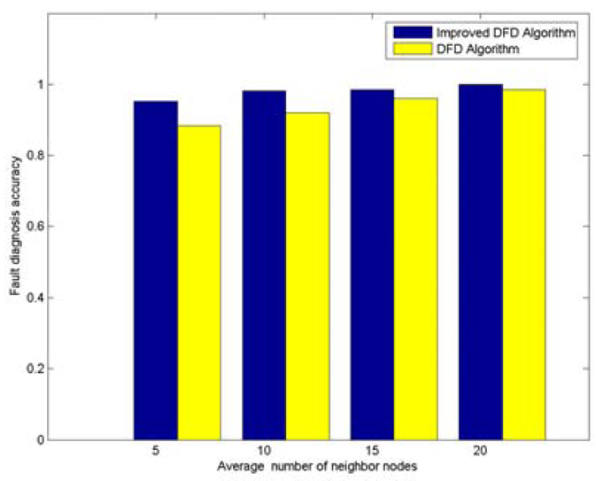
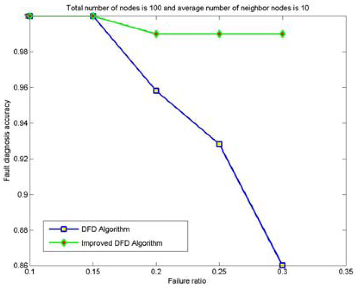
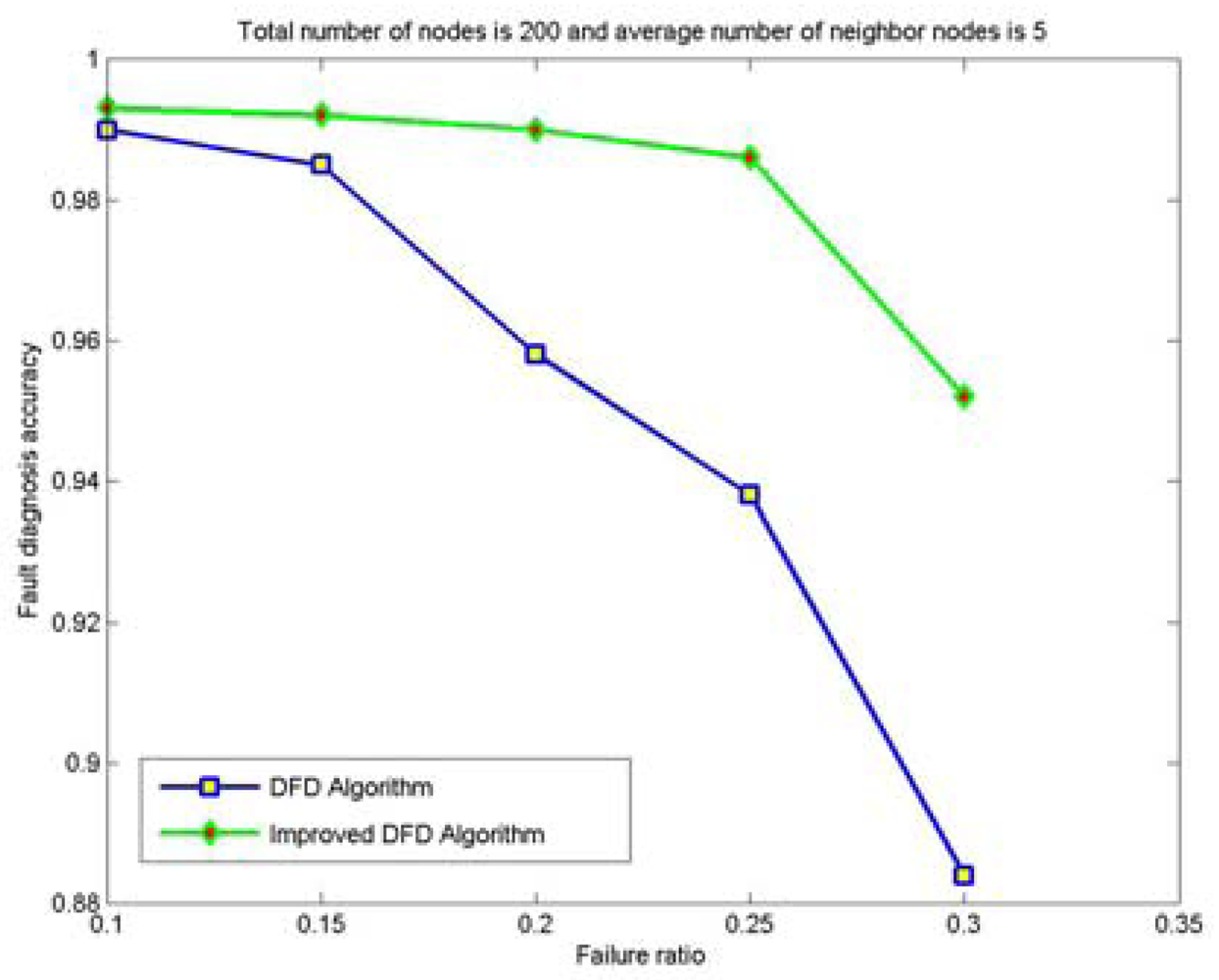
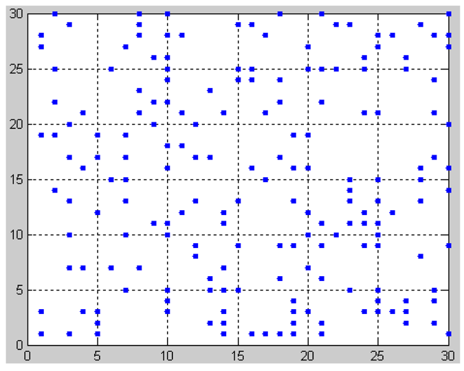
4. Simulation Examples
5. Conclusions
Acknowledgments
References and Notes
- Sun, L.M.; Li, J.Z.; Chen, Y.; Zhu, H.S. Wireless Sensor Networks; Tsinghua Publishing House: Beijing, China, 2005. [Google Scholar]
- Akyildiz, I.F.; Su, W.; Sankarasubramaniam, Y; Cayirci, E. Wireless sensor networks: a survey. Comput. Networks 2002, 38, 393–422. [Google Scholar]
- Feng, Xia. QoS Challenges and opportunities in wireless sensor/actuator networks. Sensors 2008, 8, 1099–1110. [Google Scholar]
- Xia, F.; Tian, Y.C.; Li, Y.J.; Sun, Y.X. Wireless sensor/actuator network design for mobile control applications. Sensors 2007, 7, 2157–2173. [Google Scholar]
- Chen, J.R.; Kher, S.; Somani, A. Distributed fault detection of wireless sensor networks. Proceedings of the International Conference on Mobile Computing and Networkings, Los Angeles, CA, USA; ACM: New York, USA, 2006; pp. 65–72. [Google Scholar]
- Koushanfar, F.; Potkonjak, M.; Sangiovanni-Vincentelli, A. On-line fault detection of sensor measurements. In Proceedings ofthe IEEE, Sensors; IEEE Press: Toronto, 2003; Volume 2, pp. 22–24. [Google Scholar]
- Chessa, S.; Santi, P. Comparison based system level fault diagnosis in Ad hoc networks. Proceedings ofIEEE 20th Symp. on Reliable Distributed Systems (SRDS), New Orleans; IEEE Press, 2001; pp. 257–266. [Google Scholar]
- Chessa, S.; Santi, P. Crash faults identification in wireless sensor networks. Comput. Commun. 2002, 25, 1273–1282. [Google Scholar]
- Elhadef, M.; Boukerche, A; Elkadiki, H. Performance analysis of a distributed comparison based self-diagnosis protocol for wireless ad hoc networks. Proceedings of the 9th ACM International Symposium on Modeling analysis and simulation of wireless and mobile system, NY, USA; ACM, 2006; pp. 165–172. [Google Scholar]
- Gao, J.L.; Xu, Y.J.; Li, X.W. Weighted-median based distributed fault detection for wireless sensor networks. J. Softw. 2007, 18, 1208–1217. [Google Scholar]
- Wang, T.Y.; Chang, L.Y.; Dun, D.R.; Wu, J.Y. Distributed fault-tolerant detection via sensor fault detection in sensor networks. Proceedings of the IEEE 10th International Conference on Information Fusion, Quebec, Canada; 2007; pp. 1–6. [Google Scholar]
- Krishnamachari, B.; Iyengar, S. Distributed Bayesian algorithms for fault-tolerant event region detection in wireless sensor networks. IEEE Trans. Comput. 2004, 53, 241–250. [Google Scholar]
- Wang, P.; Zheng, J.; Li, C. An Agreement-Based Fault Detection Mechanism for Under Water Sensor Networks. Proceedings of the Global Telecommunications Conference, Washington, DC; 2007; pp. 1195–1200. [Google Scholar]
- Luo, X.; Dong, M.; Huang, Y. On distributed fault-tolerant detection in wireless sensor networks. IEEE Trans. Comput. 2006, 55, 58–70. [Google Scholar]
- Lee, M.H.; Choi, Y.H. Fault detection of wireless sensor networks. Comput. Commun. 2008, 31, 3469–3475. [Google Scholar]
- Nakamura, E.F.; Figueiredo, C.M.S.; Nakamura, F.G.; Loureiro, A.A.F. Diffuse: A topology building engine for wireless sensor networks. Signal Processing 2007, 87, 2991–3009. [Google Scholar]
- Nakamura, E.F.; Loureiro, A.A.F.; Frery, A.C. Information fusion for wireless sensor networks: Methods, models, and classifications. ACM Comput. 2007, 39. No. 9. [Google Scholar]


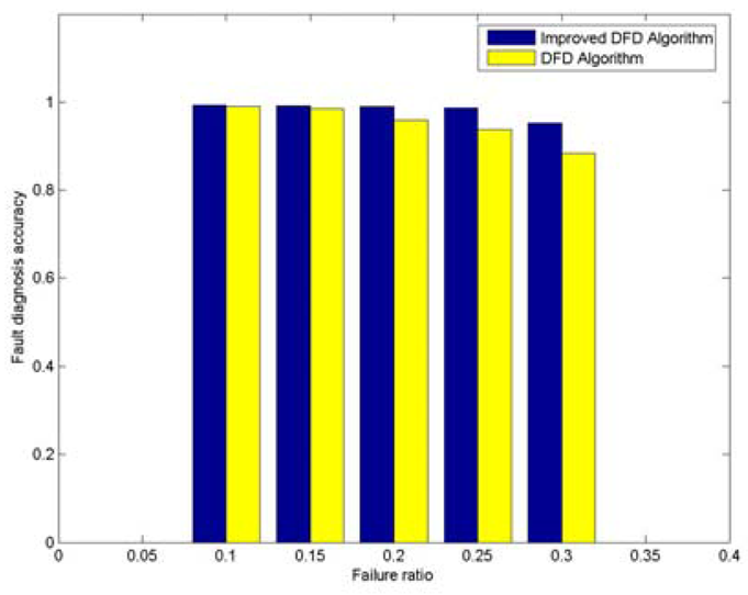
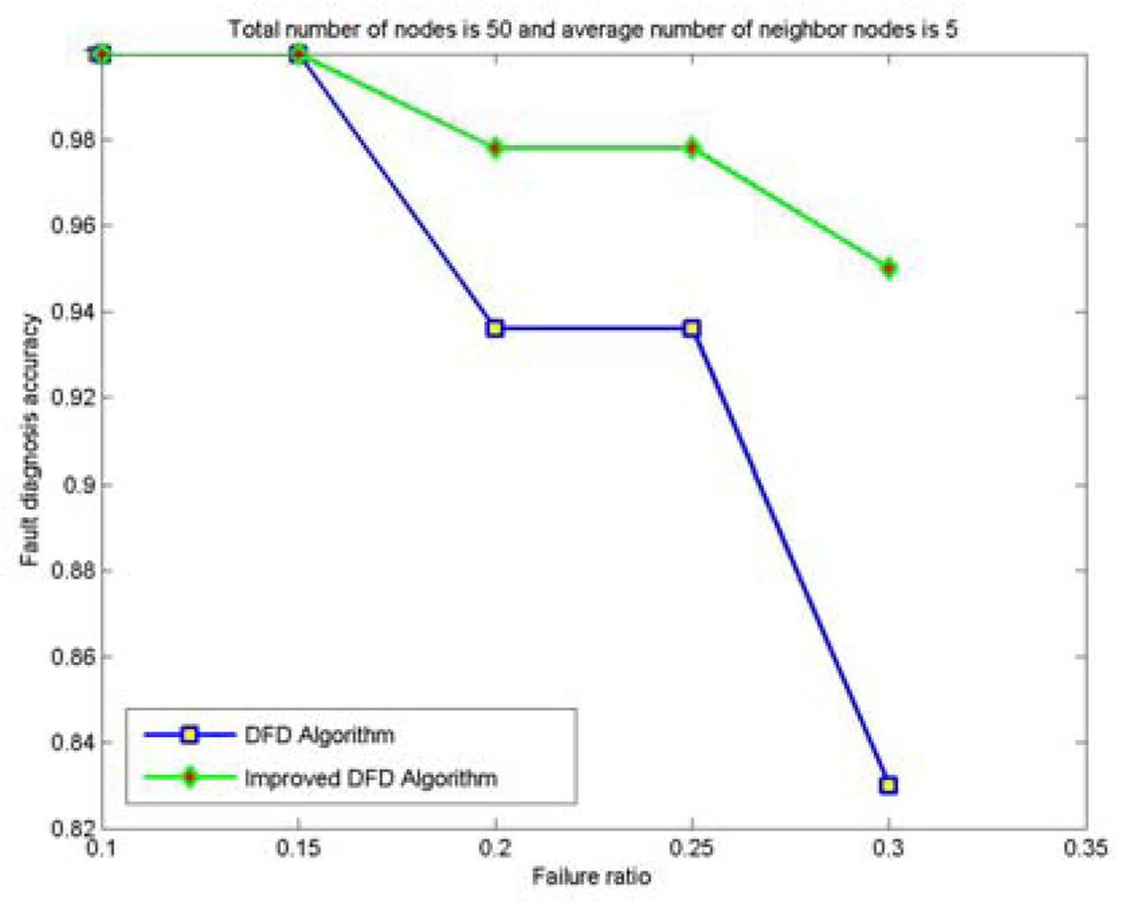
| Node's failure ratio ρ | Average number of neighbor nodes k | ||||
|---|---|---|---|---|---|
| 5 | 10 | 15 | 20 | ||
| 0.1 | 0.998 | 1 | 1 | 1 | |
| 0.15 | 0.985 | 0.992 | 1 | 1 | |
| 0.2 | 0.962 | 0.976 | 0.993 | 1 | |
| 0.25 | 0.935 | 0.955 | 0.981 | 0.992 | |
| 0.3 | 0.873 | 0.917 | 0.968 | 0.976 | |
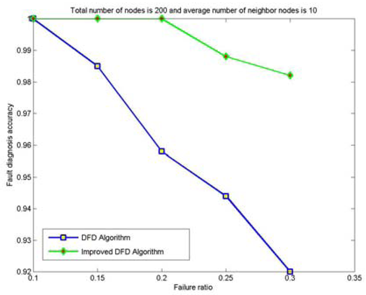
| Node's failure ratio p | Average number of neighbor nodes k | |||
|---|---|---|---|---|
| 5 | 10 | 15 | 20 | |
| 0.1 | 1 | 1 | 1 | 1 |
| 0.15 | 0.997 | 1 | 1 | 1 |
| 0.2 | 0.992 | 0.997 | 1 | 1 |
| 0.25 | 0.985 | 0.992 | 1 | 1 |
| 0.3 | 0.964 | 0.986 | 0.999 | 1 |
© 2009 by the authors; licensee Molecular Diversity Preservation International, Basel, Switzerland. This article is an open access article distributed under the terms and conditions of the Creative Commons Attribution license (http://creativecommons.org/licenses/by/3.0/).
Share and Cite
Jiang, P. A New Method for Node Fault Detection in Wireless Sensor Networks. Sensors 2009, 9, 1282-1294. https://doi.org/10.3390/s90201282
Jiang P. A New Method for Node Fault Detection in Wireless Sensor Networks. Sensors. 2009; 9(2):1282-1294. https://doi.org/10.3390/s90201282
Chicago/Turabian StyleJiang, Peng. 2009. "A New Method for Node Fault Detection in Wireless Sensor Networks" Sensors 9, no. 2: 1282-1294. https://doi.org/10.3390/s90201282
APA StyleJiang, P. (2009). A New Method for Node Fault Detection in Wireless Sensor Networks. Sensors, 9(2), 1282-1294. https://doi.org/10.3390/s90201282