
Multi-Scale Fusion Lightweight Target Detection Method for Coal and Gangue Based on EMBS-YOLOv8s


Abstract
1. Introduction
- (1)
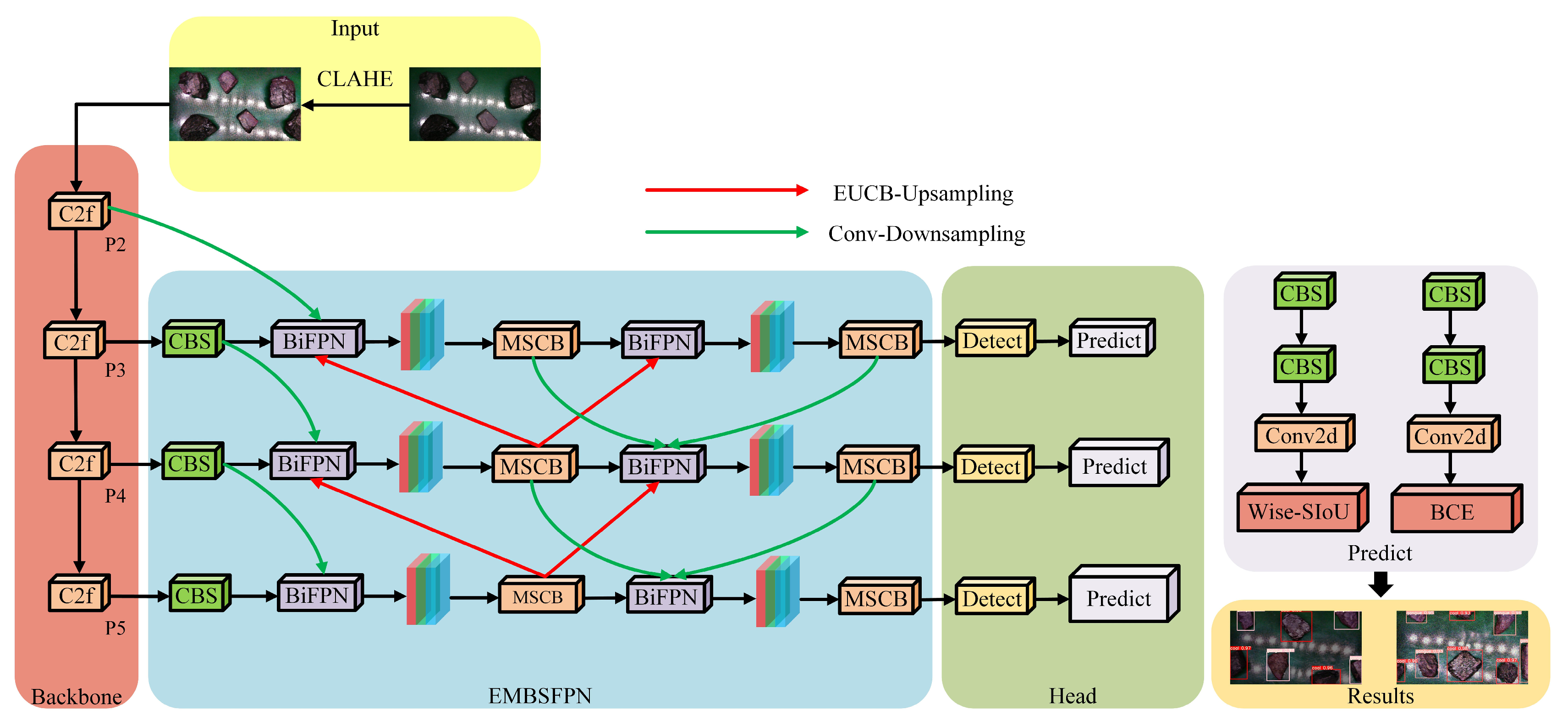
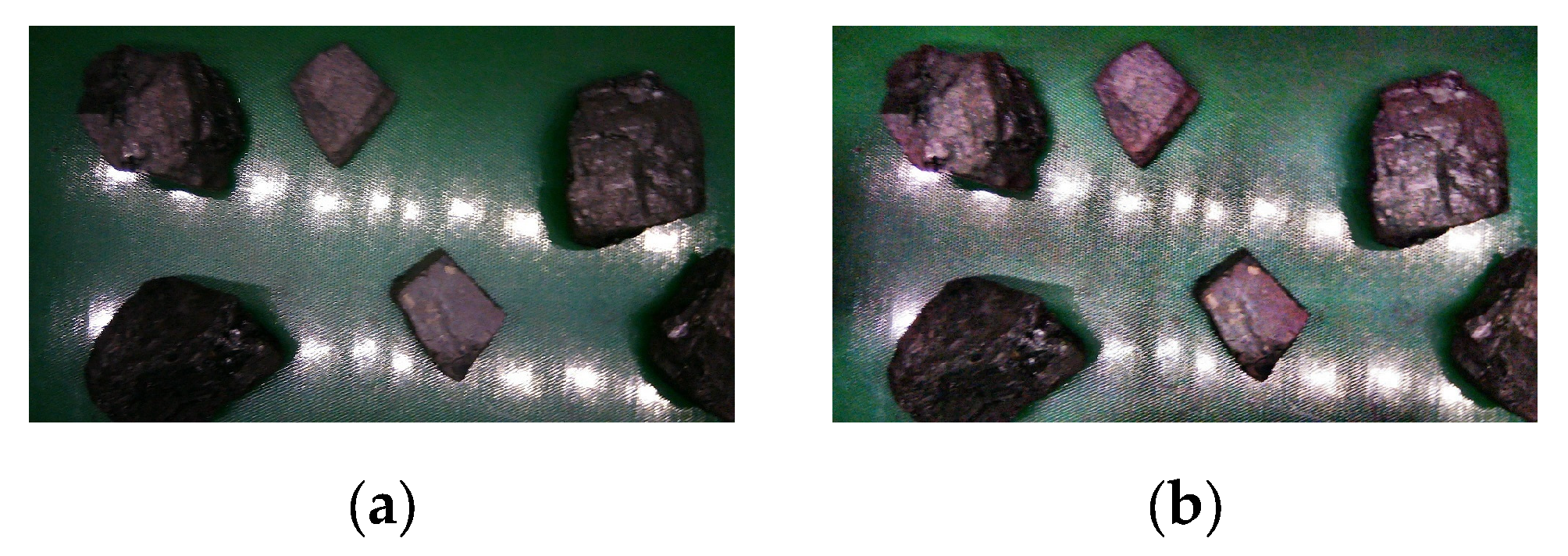
- Aiming at the problems of the low contrast and clarity of coal gangue images caused by low illumination, high conveyor belt speed, and dust interference in the coal separation environment, this paper uses Contrast-Limited Adaptive Histogram Equalization (CLAHE) to preprocess the acquired images of coal gangue to improve the quality of the images.
- (2)
- The self-designed Efficient Multi-Branch and Scale Feature Pyramid Network (EMBSFPN) is used in the neck network of the YOLOv8s model, which improves the detection accuracy of the model and also reduces the complexity of the model.
- (3)
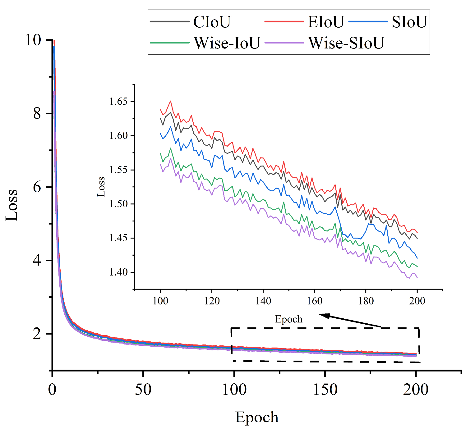
- Replacing the CIoU loss function with the Wise-SIoU function at the prediction end of the YOLOv8s model improves the convergence and stability of the model and solves the problem that there is an imbalance of hard and easy samples in the dataset.
2. EMBS-YOLOv8s Model
2.1. Improvements to the Neck Network
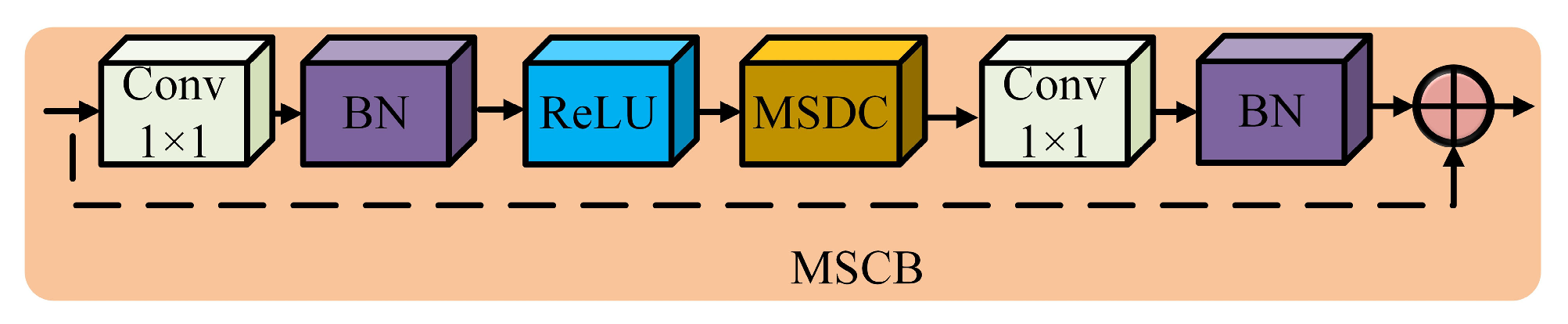
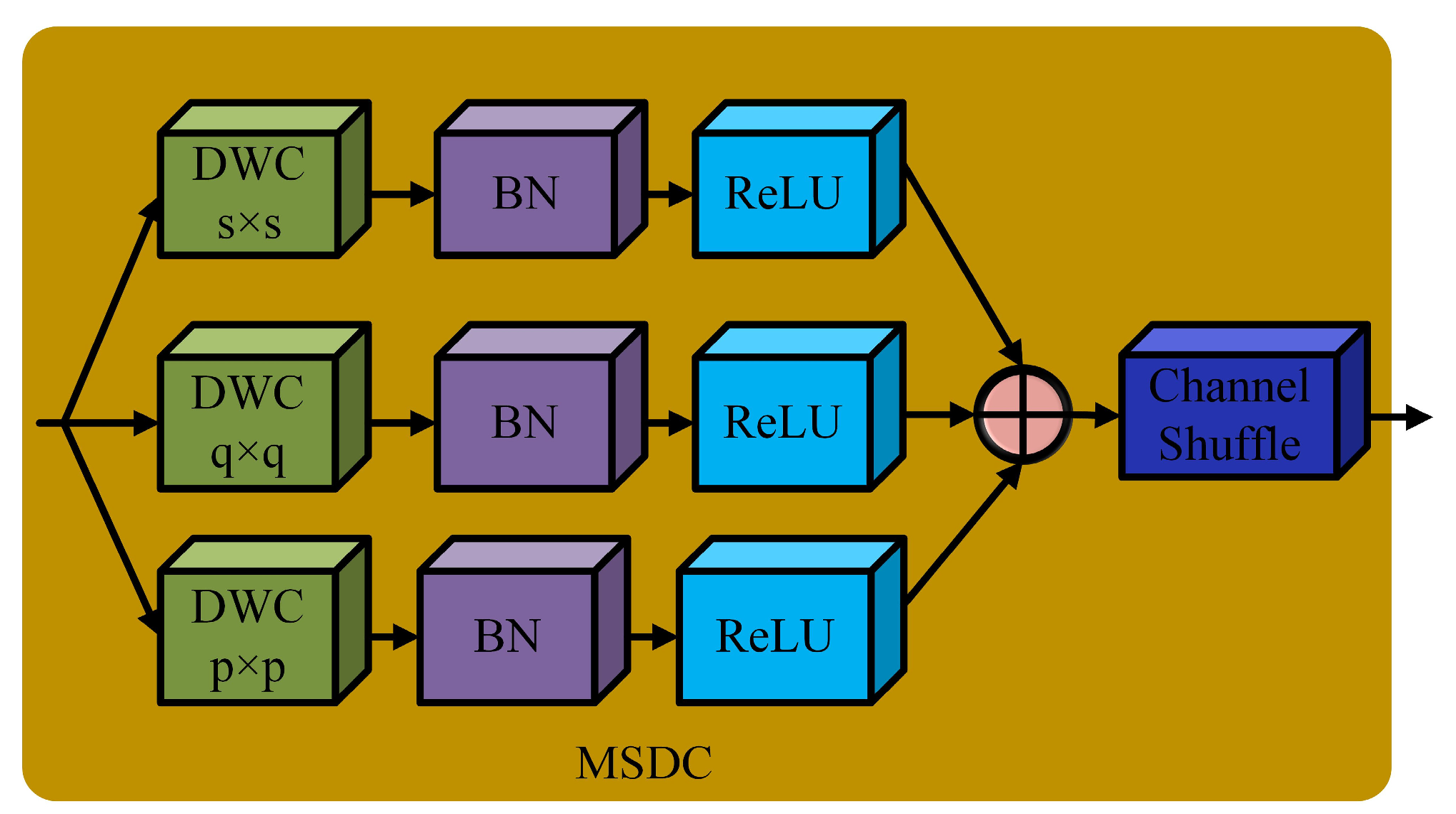
2.1.1. Multi-Scale Convolution Block (MSCB)
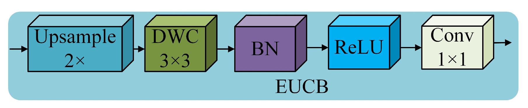
2.1.2. Efficient Up-Convolution Block (EUCB)
2.2. Improvement of Loss Function
3. Image Acquisition and Preprocessing of Coal Gangue
3.1. Image Acquisition Platform for Coal Gangue
3.2. Image Acquisition of Coal Gangue
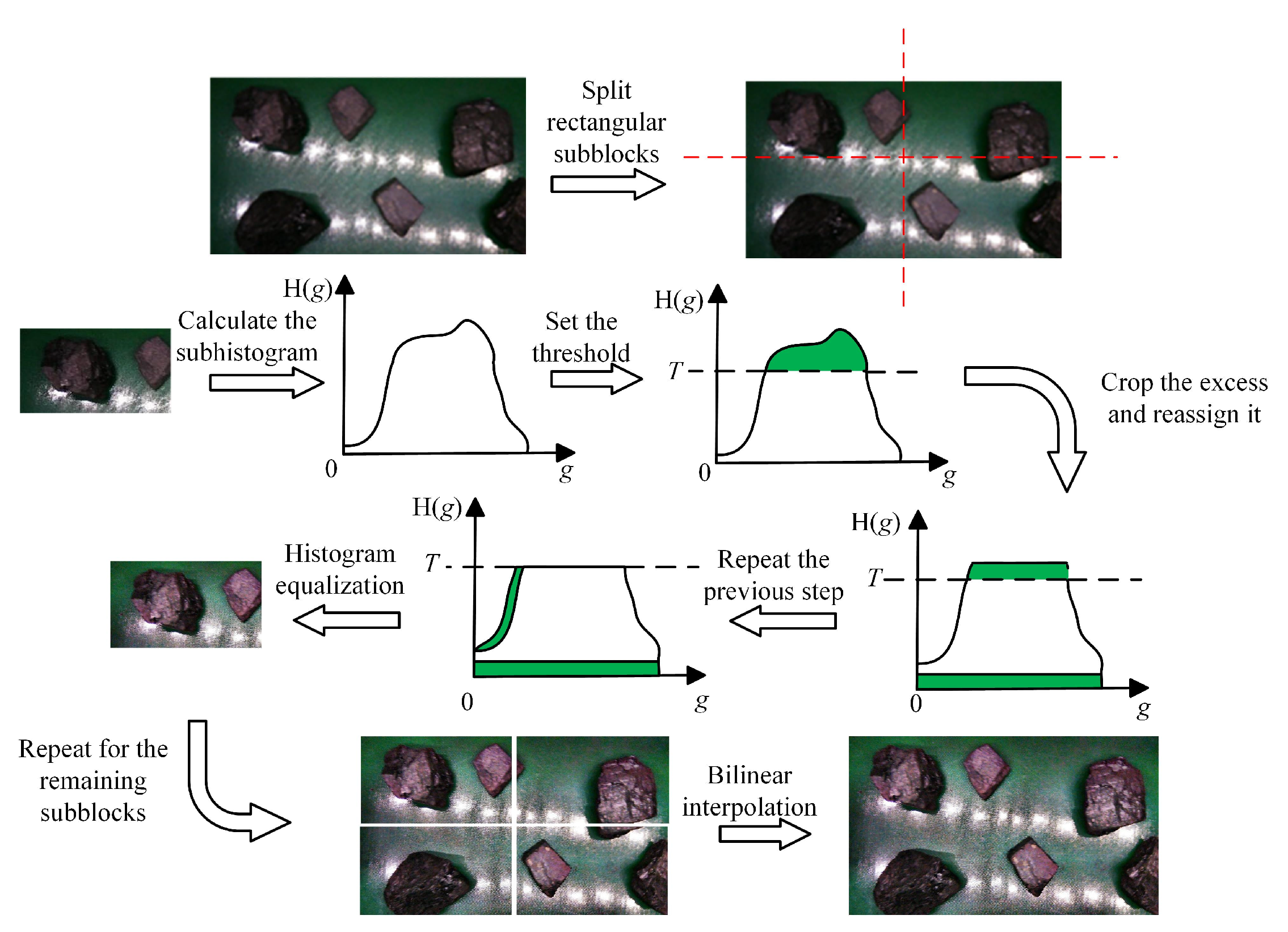
3.3. Image Preprocessing for Coal Gangue
- Divide the input image into equal and non-overlapping subblocks (the size is usually in pixels).
- Calculate the histogram H(g) of each subblock separately. (g indicates the gray level of the current subblock area.)
- Set a threshold, T, for the histogram calculated by each sub-block. A histogram’s gray levels that surpass the threshold are clipped, and the portion that does so is then divided equally among all the histogram’s gray levels. The formula for calculating the threshold T is
- 4.
- Perform histogram equalization on the trimmed sub-blocks.
- 5.
- The gray value of pixels is reconstructed by a bilinear interpolation algorithm.
4. Experimental Environment Configuration and Evaluation Indicators
4.1. Experimental Environment Configuration
4.2. Evaluation Indicators
5. Experimental Results and Analysis
5.1. Experimental Results of Different Neck Networks
5.2. Experimental Results of Different Loss Functions
5.3. Ablation Experiment
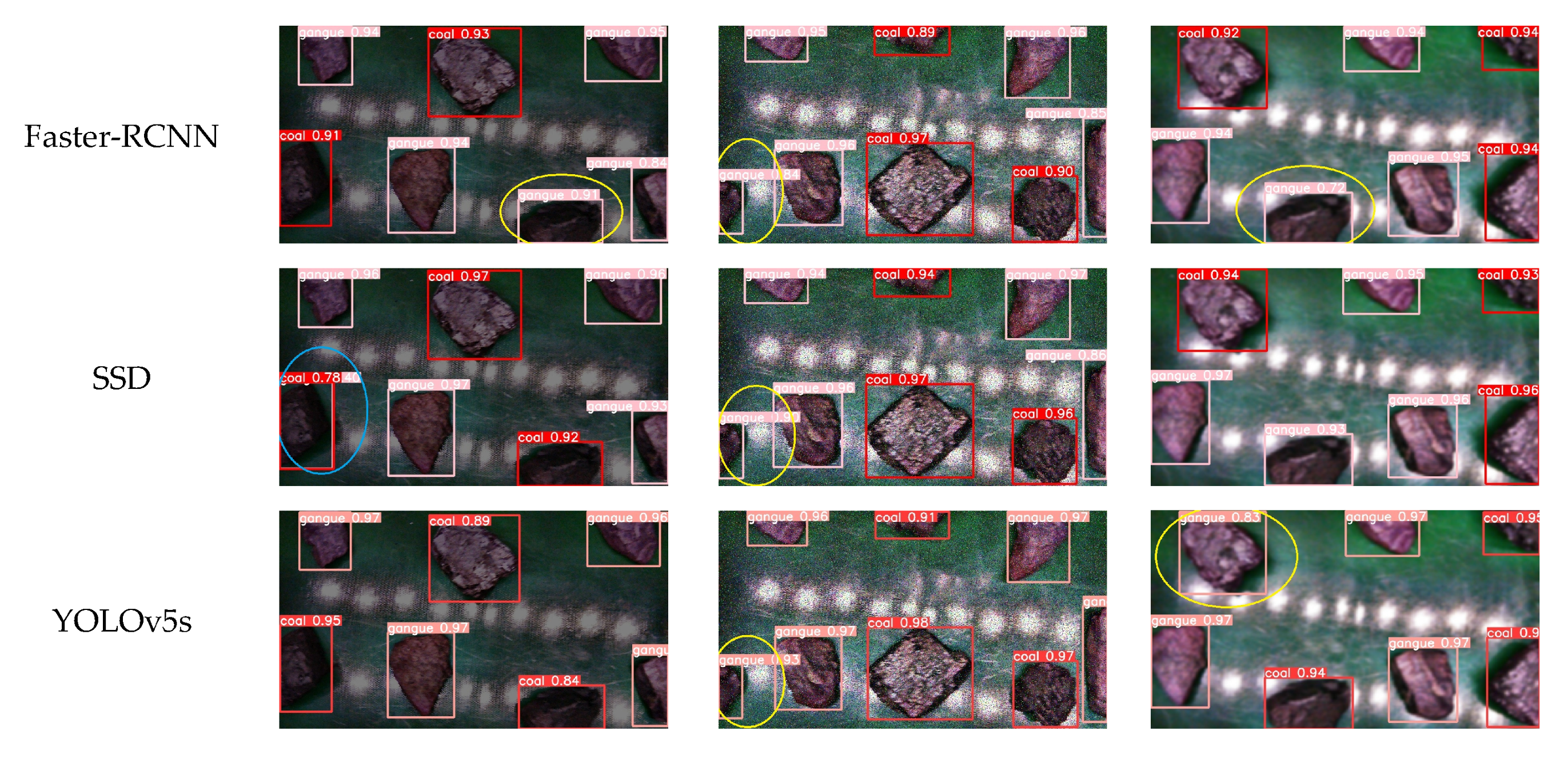
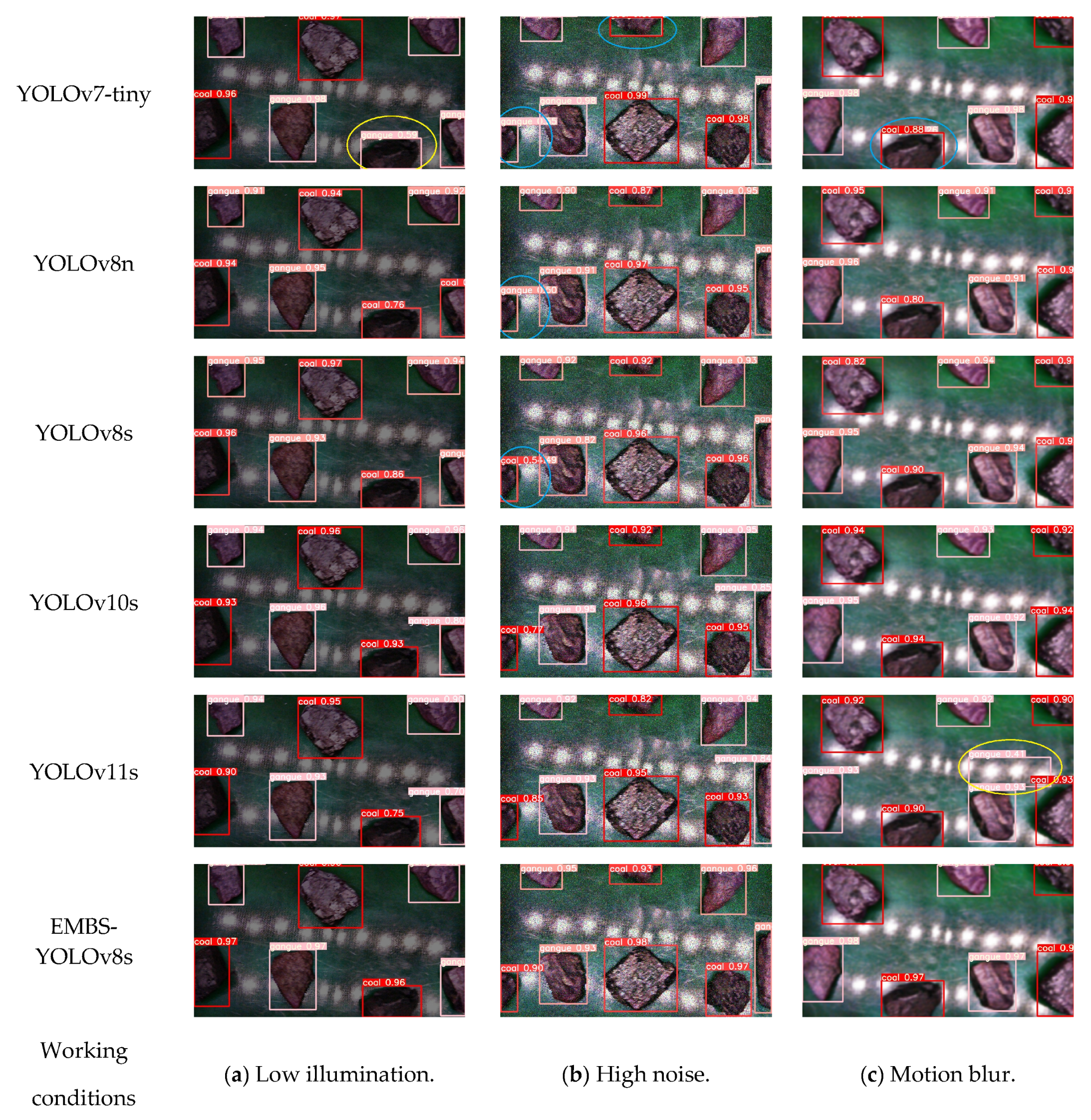
5.4. Comparative Experiment
6. Conclusions
- (1)
- A coal gangue detection method based on the EMBS-YOLOv8s model is proposed in this paper. By preprocessing the image with CLAHE, the coal gangue image’s clarity and contrast are enhanced. The EMBSFPN structure replaces the original PAN-FPN structure, increasing detection accuracy while decreasing model complexity. The CIoU loss function is improved with the Wise-SIoU loss function; this fixes the imbalance of hard- and easy-to-detect samples in the dataset in addition to enhancing the model’s convergence and stability.
- (2)
- The experimental results show that the average detection accuracy of the EMBS-YOLOv8s model on the self-constructed coal gangue dataset reached 96.0%, which was 2.1% higher than that of the original YOLOv8s model; the number of parameters, computation, and volume of the model were also reduced by 29.59%, 12.68%, and 28.44%, respectively, relative to those of the original YOLOv8s model. Meanwhile, compared with other YOLO series models, the EMBS-YOLOv8s model had high accuracy, low complexity, and better detection speed, and, at the same time, it could also effectively avoid the occurrence of misdetection and omission in complex scenes such as those with low illumination, low noise, and motion blur.
- (3)
- In future work, we will continue to aim at the coexistence of the lightweight characteristic and high accuracy of the model and study a model that can be deployed in the coal gangue sorting robotic system to verify its performance in the actual intelligent sorting of coal gangue. In addition, if we consider the fusion of visible, infrared, or multispectral images to form a multimodal feature for the model to learn in the future, it will effectively improve the accuracy of the detection of coal gangue in different environments.
Author Contributions
Funding
Institutional Review Board Statement
Informed Consent Statement
Data Availability Statement
Conflicts of Interest
References
- Raza, M.A.; Karim, A.; Aman, M.; Al-Khasawneh, M.A.; Faheem, M. Global progress towards the Coal: Tracking coal reserves, coal prices, electricity from coal, carbon emissions and coal phase-out. Gondwana Res. 2025, 139, 43–72. [Google Scholar] [CrossRef]
- Hower, J.C.; Finkelman, R.B.; Eble, C.F.; Arnold, B.J. Understanding coal quality and the critical importance of comprehensive coal analyses. Int. J. Coal Geol. 2022, 263, 104120. [Google Scholar] [CrossRef]
- Li, J.; Wang, J. Comprehensive utilization and environmental risks of coal gangue: A review. J. Clean. Prod. 2019, 239, 117946. [Google Scholar] [CrossRef]
- Zhu, T.; Wu, X.; Xing, C.; Ju, Q.; Su, S. Current situation and progress of coal gangue resource utilization. Coal Sci. Technol. 2024, 52, 380–390. [Google Scholar] [CrossRef]
- Wang, S.; Luo, K.; Wang, X.; Sun, Y. Estimate of sulfur, arsenic, mercury, fluorine emissions due to spontaneous combustion of coal gangue: An important part of Chinese emission inventories. Environ. Pollut. 2016, 209, 107–113. [Google Scholar] [CrossRef]
- Jiang, Z.; He, K.; Zhang, D. A review of intelligent coal gangue separation technology and equipment development. Int. J. Coal Prep. Util. 2023, 44, 1308–1324. [Google Scholar] [CrossRef]
- Zhao, G.; Chang, F.; Chen, J.; Si, G. Research and prospect of underground intelligent coal gangue sorting technology: A review. Miner. Eng. 2024, 215, 108818. [Google Scholar] [CrossRef]
- Wang, W.; Lv, Z.; Lu, H. Research on methods to differentiate coal and gangue using image processing and a support vector machine. Int. J. Coal Prep. Util. 2021, 41, 603–616. [Google Scholar] [CrossRef]
- Zhou, J.; Guo, Y.; Wang, S.; Cheng, G. Research on intelligent optimization separation technology of coal and gangue base on LS-FSVM by using a binary artificial sheep algorithm. Fuel 2022, 319, 123837. [Google Scholar] [CrossRef]
- Wang, D.; Ni, J.; Du, T. An image recognition method for coal gangue based on ASGS-CWOA and BP neural network. Symmetry 2022, 14, 880. [Google Scholar] [CrossRef]
- Xue, G.; Li, X.; Qian, X.; Zhang, Y. Coal-gangue image recognition in fully-mechanized caving face based on random forest. Ind. Mine Autom. 2020, 46, 57–62. [Google Scholar] [CrossRef]
- Gomez-Flores, A.; Ilyas, S.; Heyes, G.W.; Kim, H. A critical review of artificial intelligence in mineral concentration. Miner. Eng. 2022, 189, 107884. [Google Scholar] [CrossRef]
- McCoy, J.T.; Auret, L. Machine learning applications in minerals processing: A review. Miner. Eng. 2019, 132, 95–109. [Google Scholar] [CrossRef]
- Gao, L.; Yu, P.; Dong, H.; Liang, C.; Zhang, Z. Review of coal gangue recogntion methods of based on machine vision. Sci. Technol. Eng. 2024, 24, 11039–11049. [Google Scholar] [CrossRef]
- Wang, S.; Zhu, J.; Li, Z.; Sun, X.; Wang, G. Coal gangue target detection based on improved YOLOv5s. Appl. Sci. 2023, 13, 11220. [Google Scholar] [CrossRef]
- Yan, P.; Sun, Q.; Yin, N.; Hua, L.; Shang, S.; Zhang, C. Detection of coal and gangue based on improved YOLOv5.1 which embedded scSE module. Measurement 2022, 188, 110530. [Google Scholar] [CrossRef]
- Wu, L.; Zhang, L.; Chen, L.; Shi, J.; Wan, J. A lightweight and multisource information fusion method for real-time monitoring of lump coal on mining conveyor belts. Int. J. Intell. Syst. 2023, 2023, 5327122. [Google Scholar] [CrossRef]
- Shan, P.F.; Sun, H.; Lai, X.; Zhu, X.; Yang, J.; Gao, J. Identification method on mixed and release state of coal-gangue masses of fully mechanized caving based on improved Faster R-CNN. J. China Coal Soc. 2022, 47, 1382–1394. [Google Scholar] [CrossRef]
- Gao, Y.; Zhang, B.; Lang, L. Coal and gangue recognition technology and implementation based on deep learning. Coal Sci. Technol. 2021, 49, 202–208. [Google Scholar]
- Zhang, L.; Sun, Z.; Tao, H.; Wang, J.; Yi, W. Integration of lightweight network and attention mechanism for the coal and gangue recognition method. Min. Metall. Explor. 2025, 42, 191–204. [Google Scholar] [CrossRef]
- Mao, Q.; Li, S.; Hu, X.; Xue, X.; Yao, L. Foreign object recognition of belt conveyor in coal mine based on improved YOLOv7. Ind. Mine Autom. 2022, 48, 26–32. [Google Scholar] [CrossRef]
- Xin, F.; Jia, Q.; Yang, Y.; Pan, H.; Wang, Z. A high accuracy detection method for coal and gangue with S3DD-YOLOv8. Int. J. Coal Prep. Util. 2024, 45, 637–655. [Google Scholar] [CrossRef]
- Fan, Y.; Mao, S.; Li, M.; Wu, Z.; Kang, J. CM-YOLOv8: Lightweight YOLO for coal mine fully mechanized mining face. Sensors 2024, 24, 1866. [Google Scholar] [CrossRef] [PubMed]
- Cao, Y.; Cao, Q.; Qian, C.; Chen, D. YOLO-AMM: A Real-Time Classroom Behavior Detection Algorithm Based on Multi-Dimensional Feature Optimization. Sensors 2025, 25, 1142. [Google Scholar] [CrossRef]
- Rahman, M.M.; Munir, M.; Marculescu, R. Emcad: Efficient multi-scale convolutional attention decoding for medical image segmentation. In Proceedings of the 2024 IEEE Conference on Computer Vision and Pattern Recognition (CVPR), Seattle, WA, USA, 17–21 June 2024; pp. 11769–11779. [Google Scholar] [CrossRef]
- Sandler, M.; Howard, A.; Zhu, M.; Zhmoginov, A.; Chen, L. Mobilenetv2: Inverted residuals and linear bottlenecks. In Proceedings of the 2018 IEEE Conference on Computer Vision and Pattern Recognition (CVPR), Salt Lake City, UT, USA, 18–22 June 2018; pp. 4510–4520. [Google Scholar] [CrossRef]
- Zhang, X.; Zhou, X.; Lin, M.; Sun, J. Shufflenet: An extremely efficient convolutional neural network for mobile devices. In Proceedings of the 2018 IEEE Conference on Computer Vision and Pattern Recognition (CVPR), Salt Lake City, UT, USA, 18–22 June 2018; pp. 6848–6856. [Google Scholar] [CrossRef]
- Chen, Y.; Yuan, X.; Wang, J.; Wu, R.; Li, X.; Hou, Q.; Cheng, M.-M. YOLO-MS: Rethinking multi-scale representation learning for real-time object detection. IEEE Trans. Pattern Anal. Mach. Intell. 2025, 99, 1–14. [Google Scholar] [CrossRef]
- Du, S.; Zhang, B.; Zhang, P.; Xiang, P. An improved bounding box regression loss function based on CIOU loss for multi-scale object detection. In Proceedings of the 2021 IEEE 2nd International Conference on Pattern Recognition and Machine Learning (PRML 2021), Chengdu, China, 16–18 July 2021; pp. 92–98. [Google Scholar] [CrossRef]
- Tong, Z.; Chen, Y.; Xu, Z.; Yu, R. Wise-IoU: Bounding box regression loss with dynamic focusing mechanism. arXiv 2023, arXiv:2301.10051. [Google Scholar] [CrossRef]
- Fan, H.; Liu, J.; Cao, X.; Zhang, C.; Zhang, X.; Li, M.; Ma, H.; Mao, Q. Multi-scale target intelligent detection method for coal, foreign object and early damage of conveyor belt surface under low illumination and dust fog. J. China Coal Soc. 2024, 49, 1259–1270. [Google Scholar] [CrossRef]
- Yan, J.; Jia, X.; Sui, G.; Tu, J. Study on image definition evaluation function. Opt. Instrum. 2019, 41, 54–58. [Google Scholar]
- Yang, Z.; Guan, Q.; Zhao, K.; Yang, J.; Xu, X.; Long, H.; Tang, Y. Multi-branch Auxiliary Fusion YOLO with Re-parameterization Heterogeneous Convolutional for Accurate Object Detection. In Proceedings of the Chinese Conference on Pattern Recognition and Computer Vision (PRCV), Singapore, 18 October 2024; pp. 492–505. [Google Scholar] [CrossRef]
- Li, D.; Wang, G.; Guo, Y.; Wang, S.; Yang, Y. Image recognition method of coal gangue in complex workingconditions based on CES-YOLO algorithm. Coal Sci. Technol. 2024, 52, 226–237. [Google Scholar] [CrossRef]
- Zhang, Y.-F.; Ren, W.; Zhang, Z.; Jia, Z.; Wang, L.; Tan, T. Focal and efficient IOU loss for accurate bounding box regression. Neurocomputing 2022, 506, 146–157. [Google Scholar] [CrossRef]


| Evaluation Indicators | Original Image of Coal Gangue | Image of Coal Gangue After CLAHE Processing |
|---|---|---|
| Laplacian | 1029.69 | 4103.82 |
| Mean and Variance | 1.48—brightness is too dark | 0.84—brightness normal |
| Name | Configuration |
|---|---|
| Operating system | Windows11 |
| Python | 3.8.2 |
| Pytorch | 2.0.1 |
| CUDA | 11.8 |
| CuDNN | 11.8 |
| Neck Network | mAP/% | F1/% | Params/M |
|---|---|---|---|
| Original structure | 93.9 | 87.15 | 11,126,358 |
| MAFPN | 94.6 | 88.69 | 11,190,838 |
| BiFPN | 94.9 | 89.71 | 7,365,090 |
| EMBSFPN | 95.8 | 90.19 | 7,834,599 |
| IOU Loss Functions | mAP/% | F1/% |
|---|---|---|
| CIoU | 95.8 | 90.19 |
| EIoU | 94.3 | 88.05 |
| SIoU | 95.0 | 88.62 |
| Wise-IoU | 95.1 | 89.35 |
| Wise-SIoU | 96.0 | 90.25 |
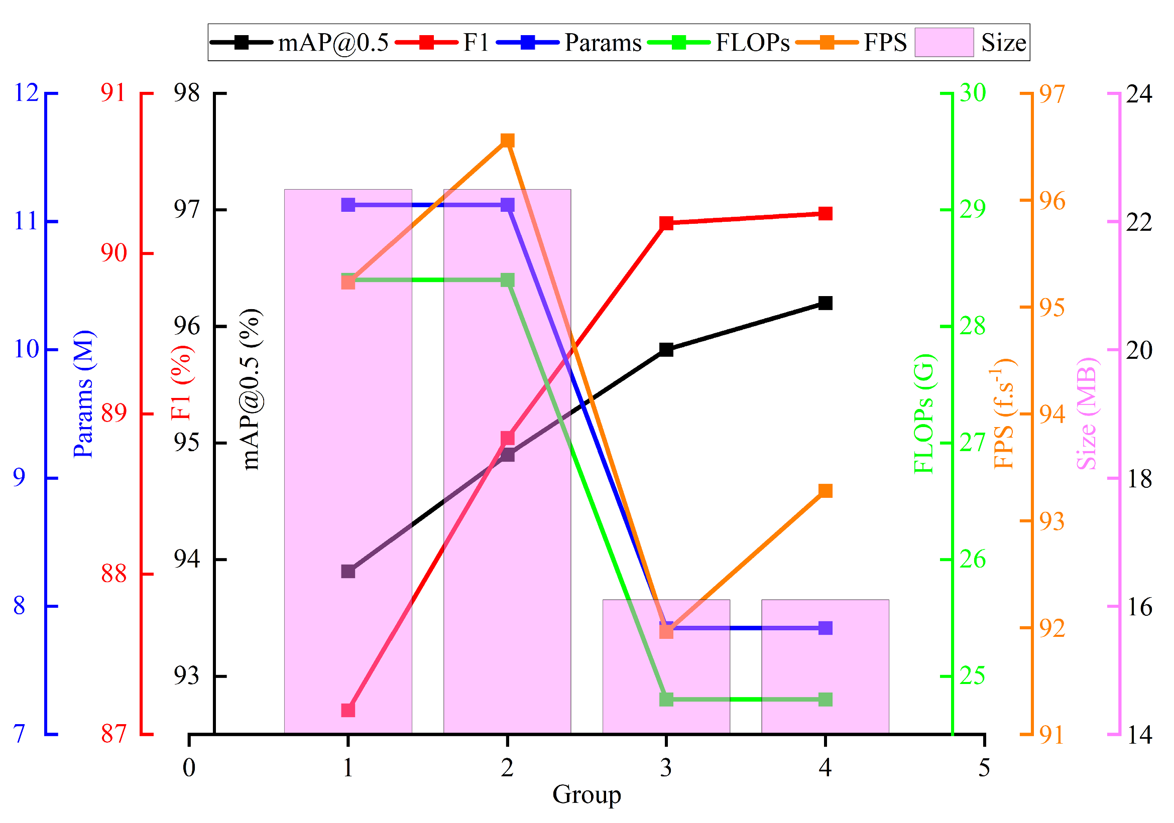
| Group | 1 | 2 | 3 | 4 |
|---|---|---|---|---|
| CLAHE | √ | √ | √ | |
| EMBSFPN | √ | √ | ||
| Wise-SIOU | √ | |||
| mAP/% | 93.9 | 94.9 | 95.8 | 96.0 |
| F1/% | 87.15 | 88.85 | 90.19 | 90.25 |
| Params/M | 11,126,358 | 11,126,358 | 7,834,599 | 7,834,599 |
| FLOPs/G | 28.4 | 28.4 | 24.8 | 24.8 |
| Size/MB | 22.5 | 22.5 | 16.1 | 16.1 |
| FPS/f.s−1 | 95.23 | 96.56 | 91.96 | 93.28 |
| Model | mAP/% | F1/% | Params/M | FLOPs/G | Model Size/MB | FPS/f.s−1 |
|---|---|---|---|---|---|---|
| Faster-RCNN-Resnet50 | 92.9 | 85.55 | 41,755,286 | 134.38 | 108.10 | 23.21 |
| SSD-Vgg | 90.6 | 79.38 | 35,641,826 | 34.86 | 91.09 | 80.17 |
| YOLOv5s | 93.0 | 86.32 | 7,015,519 | 15.8 | 14.5 | 88.91 |
| YOLOv7-tiny | 88.5 | 82.06 | 6,010,302 | 13.0 | 12.3 | 102.15 |
| YOLOv8n | 93.5 | 86.84 | 3,006,038 | 8.4 | 6.3 | 98.34 |
| YOLOv8s | 93.9 | 87.15 | 11,126,358 | 28.4 | 22.5 | 95.23 |
| YOLOv10s | 92.7 | 86.50 | 8,036,508 | 24.4 | 16.6 | 91.45 |
| YOLOv11s | 91.0 | 85.13 | 9,413,574 | 21.3 | 19.2 | 86.70 |
| EMBS-YOLOv8s | 96.0 | 90.25 | 7,834,599 | 24.8 | 16.1 | 93.28 |
Disclaimer/Publisher’s Note: The statements, opinions and data contained in all publications are solely those of the individual author(s) and contributor(s) and not of MDPI and/or the editor(s). MDPI and/or the editor(s) disclaim responsibility for any injury to people or property resulting from any ideas, methods, instructions or products referred to in the content. |
© 2025 by the authors. Licensee MDPI, Basel, Switzerland. This article is an open access article distributed under the terms and conditions of the Creative Commons Attribution (CC BY) license (https://creativecommons.org/licenses/by/4.0/).
Share and Cite
Gao, L.; Yu, P.; Dong, H.; Wang, W. Multi-Scale Fusion Lightweight Target Detection Method for Coal and Gangue Based on EMBS-YOLOv8s. Sensors 2025, 25, 1734. https://doi.org/10.3390/s25061734
Gao L, Yu P, Dong H, Wang W. Multi-Scale Fusion Lightweight Target Detection Method for Coal and Gangue Based on EMBS-YOLOv8s. Sensors. 2025; 25(6):1734. https://doi.org/10.3390/s25061734
Chicago/Turabian StyleGao, Lin, Pengwei Yu, Hongjuan Dong, and Wenjie Wang. 2025. "Multi-Scale Fusion Lightweight Target Detection Method for Coal and Gangue Based on EMBS-YOLOv8s" Sensors 25, no. 6: 1734. https://doi.org/10.3390/s25061734
APA StyleGao, L., Yu, P., Dong, H., & Wang, W. (2025). Multi-Scale Fusion Lightweight Target Detection Method for Coal and Gangue Based on EMBS-YOLOv8s. Sensors, 25(6), 1734. https://doi.org/10.3390/s25061734