
Enhancing Semi-Supervised Semantic Segmentation of Remote Sensing Images via Feature Perturbation-Based Consistency Regularization Methods


Abstract
1. Introduction
- We have introduced a new semi-supervised segmentation framework for remote sensing images. The framework integrates consistency regularization and contrastive learning, enhancing the disturbances at the data and feature levels, and improves feature classification performance through contrastive learning. In addition, this method achieves state-of-the-art performance in popular segmentation benchmarks.
- We proposed a new consistency regularization method based on MT [8]. By enhancing perturbations at the feature level, the difficulty of maintaining the consistency of image features increases, thus adding to the training difficulty and improving the generalization ability of complex images. Feature perturbations plays a key role in this process and help the model to learn from more challenging features.
- We utilize contrastive learning at the feature level to achieve a better divide and category selection for the features. A threshold for entropy is established to aid in feature selection, sifting out more accurate negative samples.
2. Related Works
2.1. Supervised Semantic Segmentation
2.2. Semi-Supervised Semantic Segmentation
2.3. Semi-Supervised Semantic Segmentation of Aerial Imagery
3. Materials and Methods
3.1. Methods
3.1.1. Feature Disturbed Mean Teacher Model (FDMT)
3.1.2. Contrastive Learning with Entropy Threshold Assisted Feature Sampling
3.2. Datasets
3.2.1. iSAID
3.2.2. Potsdam
3.3. Evaluation Metrics
3.4. Implementation Detail
4. Results and Discussion
4.1. Comparison Experiments
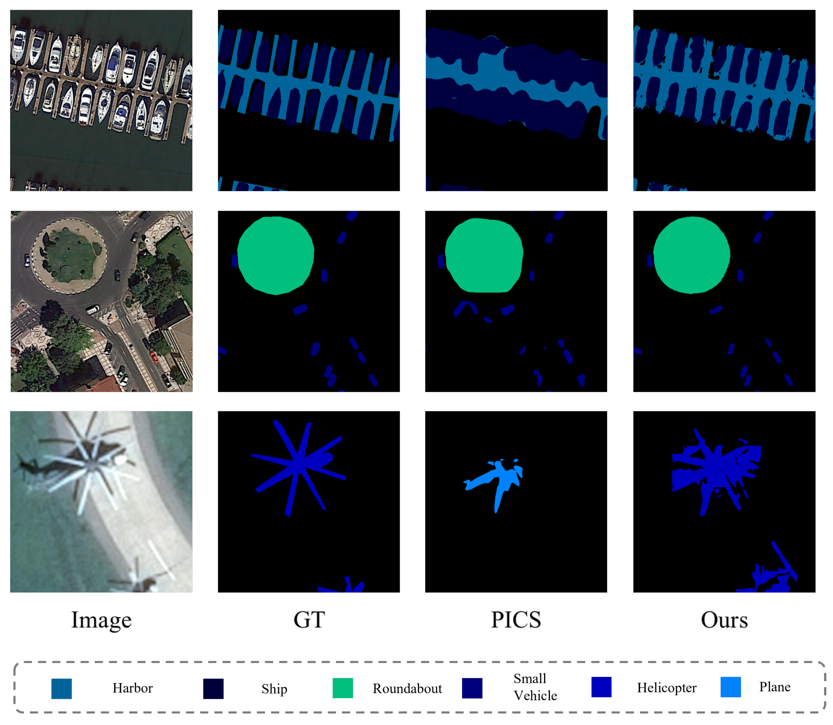
4.1.1. iSAID
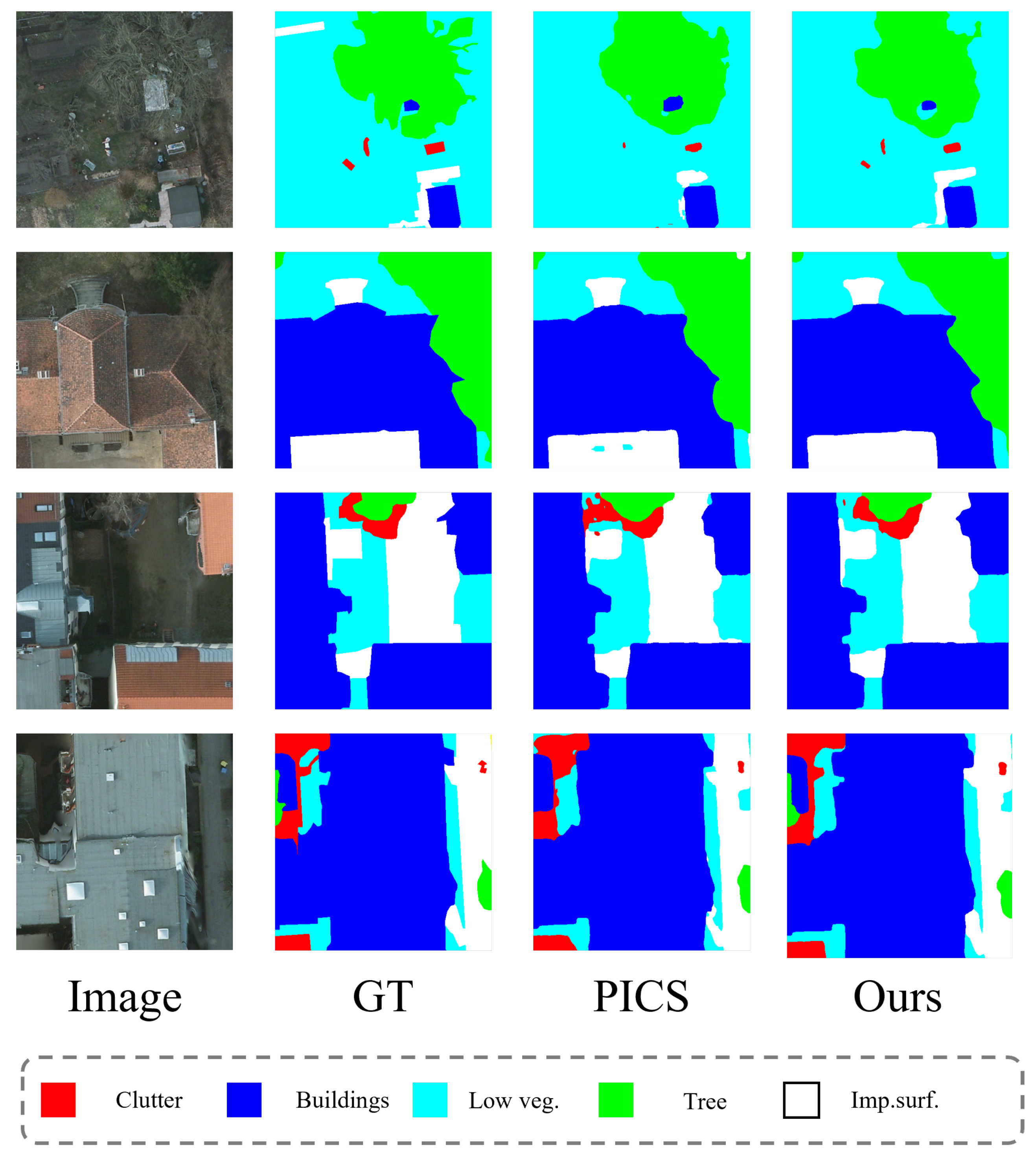
4.1.2. Potsdam
4.2. Ablation Study
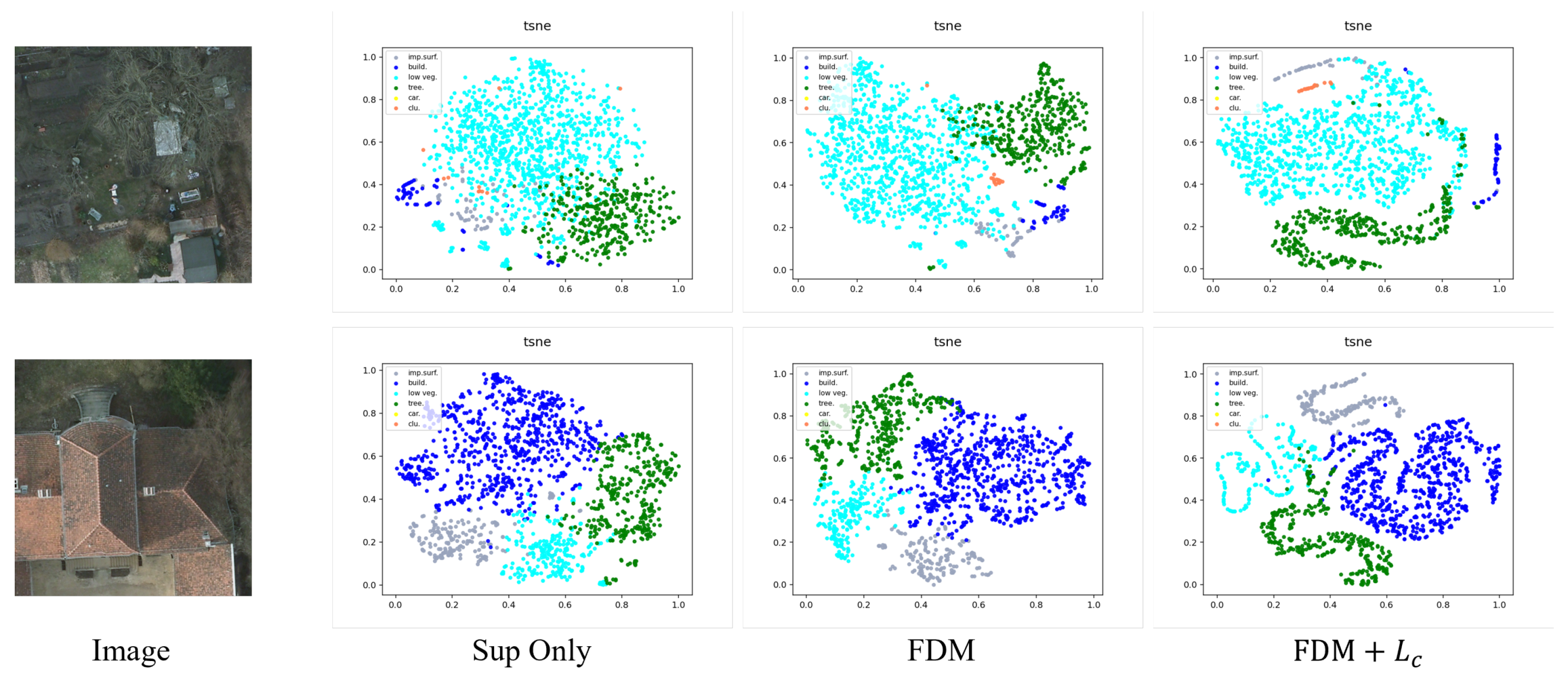
4.2.1. Ablation Study of FDM
4.2.2. Ablation Study of the Entropy Threshold
5. Conclusions
Author Contributions
Funding
Institutional Review Board Statement
Informed Consent Statement
Data Availability Statement
Acknowledgments
Conflicts of Interest
References
- Cheng, G.; Xie, X.; Han, J.; Guo, L.; Xia, G.S. Remote sensing image scene classification meets deep learning: Challenges, methods, benchmarks, and opportunities. IEEE J. Sel. Top. Appl. Earth Obs. Remote Sens. 2020, 13, 3735–3756. [Google Scholar] [CrossRef]
- Marmanis, D.; Schindler, K.; Wegner, J.D.; Galliani, S.; Datcu, M.; Stilla, U. Classification with an edge: Improving semantic image segmentation with boundary detection. ISPRS J. Photogramm. Remote Sens. 2018, 135, 158–172. [Google Scholar] [CrossRef]
- Mao, Y.; Chen, K.; Diao, W.; Sun, X.; Lu, X.; Fu, K.; Weinmann, M. Beyond single receptive field: A receptive field fusion-and-stratification network for airborne laser scanning point cloud classification. ISPRS J. Photogramm. Remote Sens. 2022, 188, 45–61. [Google Scholar] [CrossRef]
- Wei, H.; Zhang, Y.; Chang, Z.; Li, H.; Wang, H.; Sun, X. Oriented objects as pairs of middle lines. ISPRS J. Photogramm. Remote Sens. 2020, 169, 268–279. [Google Scholar] [CrossRef]
- Qi, X.; Mao, Y.; Zhang, Y.; Deng, Y.; Wei, H.; Wang, L. PICS: Paradigms Integration and Contrastive Selection for Semisupervised Remote Sensing Images Semantic Segmentation. IEEE Trans. Geosci. Remote Sens. 2023, 61, 1–19. [Google Scholar] [CrossRef]
- Yang, Z.; Yan, Z.; Diao, W.; Zhang, Q.; Kang, Y.; Li, J.; Li, X.; Sun, X. Label Propagation and Contrastive Regularization for Semi-supervised Semantic Segmentation of Remote Sensing Images. IEEE Trans. Geosci. Remote Sens. 2023, 61, 5609818. [Google Scholar]
- Zhang, B.; Zhang, Y.; Li, Y.; Wan, Y.; Guo, H.; Zheng, Z.; Yang, K. Semi-supervised deep learning via transformation consistency regularization for remote sensing image semantic segmentation. IEEE J. Sel. Top. Appl. Earth Obs. Remote Sens. 2022, 16, 5782–5796. [Google Scholar] [CrossRef]
- Tarvainen, A.; Valpola, H. Mean teachers are better role models: Weight-averaged consistency targets improve semi-supervised deep learning results. Adv. Neural Inf. Process. Syst. 2017, 30, 1195–1204. [Google Scholar]
- Olsson, V.; Tranheden, W.; Pinto, J.; Svensson, L. ClassMix: Segmentation-Based Data Augmentation for Semi-Supervised Learning. In Proceedings of the Workshop on Applications of Computer Vision, Montreal, BC, Canada, 11–17 October 2021. [Google Scholar]
- Yun, S.; Han, D.; Oh, S.J.; Chun, S.; Choe, J.; Yoo, Y. CutMix: Regularization Strategy to Train Strong Classifiers with Localizable Features. In Proceedings of the IEEE/CVF International Conference on Computer Vision (ICCV), Seoul, Republic of Korea, 27 October–2 November 2019; pp. 6023–6032. [Google Scholar]
- French, G.; Laine, S.; Aila, T.; Mackiewicz, M.; Finlayson, G. Semi-supervised semantic segmentation needs strong, varied perturbations. arXiv 2019, arXiv:1906.01916. [Google Scholar]
- Chen, X.; Yuan, Y.; Zeng, G.; Wang, J. Semi-Supervised Semantic Segmentation with Cross Pseudo Supervision. In Proceedings of the 2021 IEEE/CVF Conference on Computer Vision and Pattern Recognition (CVPR), Nashville, TN, USA, 20–25 June 2021; pp. 2613–2622. [Google Scholar] [CrossRef]
- Kim, J.; Min, Y.; Kim, D.; Lee, G.; Seo, J.; Ryoo, K.; Kim, S. Conmatch: Semi-supervised learning with confidence-guided consistency regularization. In Proceedings of the Computer Vision–ECCV 2022: 17th European Conference, Tel Aviv, Israel, 23–27 October 2022; Proceedings, Part XXX. Springer: Berlin/Heidelberg, Germany, 2022; pp. 674–690. [Google Scholar]
- He, K.; Fan, H.; Wu, Y.; Xie, S.; Girshick, R. Momentum contrast for unsupervised visual representation learning. In Proceedings of the IEEE/CVF Conference on Computer Vision and Pattern Recognition, Seattle, WA, USA, 14–19 June 2020; pp. 9729–9738. [Google Scholar]
- Zhang, Y.; Wu, Z.; Zhang, Y.; Guo, J.; Yang, P.; Chen, G.; Huang, Q.; Luo, P. Bootstrapping Semantic Segmentation with Regional Contrast. In Proceedings of the IEEE/CVF Conference on Computer Vision and Pattern Recognition (CVPR), Nashville, TN, USA, 20–25 June 2021; pp. 14841–14850. [Google Scholar]
- Sohn, K.; Berthelot, D.; Carlini, N.; Zhang, Z.; Zhang, H.; Raffel, C.A.; Cubuk, E.D.; Kurakin, A.; Li, C.L. Fixmatch: Simplifying semi-supervised learning with consistency and confidence. Adv. Neural Inf. Process. Syst. 2020, 33, 596–608. [Google Scholar]
- Wang, J.X.; Chen, S.B.; Ding, C.H.; Tang, J.; Luo, B. Semi-supervised semantic segmentation of remote sensing images with iterative contrastive network. IEEE Geosci. Remote Sens. Lett. 2022, 19, 1–5. [Google Scholar] [CrossRef]
- Long, J.; Shelhamer, E.; Darrell, T. Fully Convolutional Networks for Semantic Segmentation. IEEE Trans. Pattern Anal. Mach. Intell. 2015, 39, 640–651. [Google Scholar]
- Ronneberger, O.; Fischer, P.; Brox, T. U-Net: Convolutional Networks for Biomedical Image Segmentation. In Proceedings of the International Conference on Medical Image Computing and Computer-Assisted Intervention, Munich, Germany, 5–9 October 2015; Springer: Berlin/Heidelberg, Germany, 2015; pp. 234–241. [Google Scholar]
- Chen, L.C.; Zhu, Y.; Papandreou, G.; Schroff, F.; Adam, H. Encoder-Decoder with Atrous Separable Convolution for Semantic Image Segmentation. In Proceedings of the European Conference on Computer Vision (ECCV), Munich, Germany, 8–14 September 2018; pp. 801–818. [Google Scholar]
- Zhao, H.; Shi, J.; Qi, X.; Wang, X.; Jia, J. Pyramid Scene Parsing Network. In Proceedings of the IEEE Conference on Computer Vision and Pattern Recognition (CVPR), Honolulu, HI, USA, 21–26 July 2017; pp. 2881–2890. [Google Scholar]
- Wu, H.; Zhang, J.; Huang, K. FastFCN: Rethinking Dilated Convolution in the Backbone for Semantic Segmentation. In Proceedings of the IEEE/CVF International Conference on Computer Vision (ICCV), Seoul, Republic of Korea, 27 October– 2 November 2019; pp. 2634–2642. [Google Scholar]
- Tao, H.; Duan, Q.; Lu, M.; Hu, Z. Learning Discriminative Feature Representation with Pixel-level Supervision for Forest Smoke Recognition. Pattern Recognit. 2023, 143, 109761. [Google Scholar] [CrossRef]
- Strudel, R.; Garcia, R.; Laptev, I.; Schmid, C. Segmenter: Transformer for semantic segmentation. In Proceedings of the IEEE/CVF International Conference on Computer Vision, Montreal, BC, Canada, 11–17 October 2021; pp. 7262–7272. [Google Scholar]
- Chen, J.; Lu, Y.; Yu, Q.; Luo, X.; Adeli, E.; Wang, Y.; Lu, L.; Yuille, A.L.; Zhou, Y. Transunet: Transformers make strong encoders for medical image segmentation. arXiv 2021, arXiv:2102.04306. [Google Scholar]
- Xie, E.; Wang, W.; Yu, Z.; Anandkumar, A.; Alvarez, J.M.; Luo, P. SegFormer: Simple and efficient design for semantic segmentation with transformers. Adv. Neural Inf. Process. Syst. 2021, 34, 12077–12090. [Google Scholar]
- Rasmus, A.; Valpola, H.; Honkala, M.; Berglund, M.; Raiko, T. Semi-Supervised Learning with Ladder Networks. Computer Science 2015, 9 (Suppl. S1), 1–9. [Google Scholar]
- Ouali, Y.; Hudelot, C.; Tami, M. Semi-Supervised Semantic Segmentation with Cross-Consistency Training. In Proceedings of the 2020 IEEE/CVF Conference on Computer Vision and Pattern Recognition (CVPR), Seattle, WA, USA, 13–19 June 2020; pp. 12671–12681. [Google Scholar] [CrossRef]
- Ke, Z.; Qiu, D.; Li, K.; Yan, Q.; Lau, R.W. Guided collaborative training for pixel-wise semi-supervised learning. In Proceedings of the Computer Vision–ECCV 2020: 16th European Conference, Glasgow, UK, 23–28 August 2020; Proceedings, Part XIII 16. Springer: Berlin/Heidelberg, Germany, 2020; pp. 429–445. [Google Scholar]
- Zhang, H.; Cisse, M.; Dauphin, Y.N.; Lopez-Paz, D. mixup: Beyond empirical risk minimization. arXiv 2017, arXiv:1710.09412. [Google Scholar]
- French, G.; Mackiewicz, M.; Fisher, M. Self-ensembling for visual domain adaptation. arXiv 2017, arXiv:1706.05208. [Google Scholar]
- Liu, Y.; Tian, Y.; Chen, Y.; Liu, F.; Belagiannis, V.; Carneiro, G. Perturbed and Strict Mean Teachers for Semi-supervised Semantic Segmentation. In Proceedings of the 2022 IEEE/CVF Conference on Computer Vision and Pattern Recognition (CVPR), New Orleans, LA, USA, 18–24 June 2022; pp. 4248–4257. [Google Scholar] [CrossRef]
- Yang, L.; Zhuo, W.; Qi, L.; Shi, Y.; Gao, Y. St++: Make self-training work better for semi-supervised semantic segmentation. In Proceedings of the IEEE/CVF Conference on Computer Vision and Pattern Recognition, New Orleans, LA, USA, 18–24 June 2022; pp. 4268–4277. [Google Scholar]
- Hung, W.C.; Tsai, Y.H.; Liou, Y.C.; Lin, Y.Y.; Yang, M.H. Adversarial Learning for Semi-Supervised Semantic Segmentation. In Proceedings of the British Machine Vision Conference (BMVC), Newcastle, UK, 3–6 September 2018. [Google Scholar]
- Fu, X.; Peng, Y.; Liu, Y.; Lin, Y.; Gui, G.; Gacanin, H.; Adachi, F. Semi-supervised specific emitter identification method using metric-adversarial training. IEEE Internet Things J. 2023, 10, 10778–10789. [Google Scholar] [CrossRef]
- Hung, W.C.; Tsai, Y.H.; Liou, Y.T.; Lin, Y.Y.; Yang, M.H. Adversarial learning for semi-supervised semantic segmentation. arXiv 2018, arXiv:1802.07934. [Google Scholar]
- Alonso, I.; Sabater, A.; Ferstl, D.; Montesano, L.; Murillo, A.C. Semi-supervised semantic segmentation with pixel-level contrastive learning from a class-wise memory bank. In Proceedings of the IEEE/CVF International Conference on Computer Vision, Montreal, BC, Canada, 11–17 October 2021; pp. 8219–8228. [Google Scholar]
- Wang, W.; Zhou, T.; Yu, F.; Dai, J.; Konukoglu, E.; Gool, L.V. Exploring Cross-Image Pixel Contrast for Semantic Segmentation. In Proceedings of the 2021 IEEE/CVF International Conference on Computer Vision (ICCV), Montreal, BC, Canada, 11–17 October 2021; pp. 7283–7293. [Google Scholar] [CrossRef]
- Zhao, X.; Vemulapalli, R.; Mansfield, P.A.; Gong, B.; Green, B.; Shapira, L.; Wu, Y. Contrastive Learning for Label Efficient Semantic Segmentation. In Proceedings of the 2021 IEEE/CVF International Conference on Computer Vision (ICCV), Montreal, BC, Canada, 11–17 October 2021; pp. 10603–10613. [Google Scholar] [CrossRef]
- Zhou, Y.; Xu, H.; Zhang, W.; Gao, B.; Heng, P.A. C3-SemiSeg: Contrastive Semi-supervised Segmentation via Cross-set Learning and Dynamic Class-balancing. In Proceedings of the 2021 IEEE/CVF International Conference on Computer Vision (ICCV), Montreal, BC, Canada, 11–17 October 2021; pp. 7016–7025. [Google Scholar] [CrossRef]
- Chen, X.; He, K. Exploring simple siamese representation learning. In Proceedings of the IEEE/CVF Conference on Computer Vision and Pattern Recognition, Seattle, WA, USA, 14–19 June 2021; pp. 15750–15758. [Google Scholar]
- Lai, X.; Tian, Z.; Jiang, L.; Liu, S.; Zhao, H.; Wang, L.; Jia, J. Semi-supervised semantic segmentation with directional context-aware consistency. In Proceedings of the IEEE/CVF Conference on Computer Vision and Pattern Recognition, New Orleans, LA, USA, 18–24 June 2022; pp. 1205–1214. [Google Scholar]
- Yang, L.; Qi, L.; Feng, L.; Zhang, W.; Shi, Y. Revisiting weak-to-strong consistency in semi-supervised semantic segmentation. In Proceedings of the IEEE/CVF Conference on Computer Vision and Pattern Recognition, Vancouver, BC, Canada, 17–24 June 2023; pp. 7236–7246. [Google Scholar]
- Kerdegari, H.; Razaak, M.; Argyriou, V.; Remagnino, P. Urban scene segmentation using semi-supervised GAN. In Proceedings of the Image and Signal Processing for Remote Sensing XXV. International Society for Optics and Photonics, Strasbourg, France, 9–11 September 2019; Volume 11155, p. 111551H. [Google Scholar]
- Zhang, H.; Hong, H.; Zhu, Y.; Zhang, Y.; Wang, P.; Wang, L. Semi-Supervised Semantic Segmentation of SAR Images Based on Cross Pseudo-Supervision. In Proceedings of the IGARSS 2022-2022 IEEE International Geoscience and Remote Sensing Symposium, Kuala Lumpur, Malaysia, 17–22 July 2022; IEEE: Manhattan, NY, USA, 2022; pp. 1496–1499. [Google Scholar]
- Fang, B.; Li, Y.; Zhang, H.; Chan, J.C.W. Collaborative learning of lightweight convolutional neural network and deep clustering for hyperspectral image semi-supervised classification with limited training samples. ISPRS J. Photogramm. Remote Sens. 2020, 161, 164–178. [Google Scholar] [CrossRef]
- Hong, D.; Yokoya, N.; Xia, G.S.; Chanussot, J.; Zhu, X.X. X-ModalNet: A semi-supervised deep cross-modal network for classification of remote sensing data. ISPRS J. Photogramm. Remote Sens. 2020, 167, 12–23. [Google Scholar] [CrossRef] [PubMed]
- Takeru, M.; Shin-Ichi, M.; Shin, I.; Masanori, K. Virtual Adversarial Training: A Regularization Method for Supervised and Semi-Supervised Learning. IEEE Trans. Pattern Anal. Mach. Intell. 2018, 41, 1979–1993. [Google Scholar]
- Waqas Zamir, S.; Arora, A.; Gupta, A.; Khan, S.; Sun, G.; Shahbaz Khan, F.; Zhu, F.; Shao, L.; Xia, G.S.; Bai, X. isaid: A large-scale dataset for instance segmentation in aerial images. In Proceedings of the IEEE/CVF Conference on Computer Vision and Pattern Recognition Workshops, Long Beach, CA, USA, 16–17 June 2019; pp. 28–37. [Google Scholar]
- ISPRS 2D Semantic Labeling Contest-Potsdam. Available online: https://www.isprs.org/education/benchmarks/UrbanSemLab/2d-sem-label-potsdam.aspx (accessed on 1 June 2023).
- Wang, J.X.; Chen, S.B.; Ding, C.H.; Tang, J.; Luo, B. RanPaste: Paste consistency and pseudo label for semisupervised remote sensing image semantic segmentation. IEEE Trans. Geosci. Remote Sens. 2021, 60, 1–16. [Google Scholar] [CrossRef]


| Method | 1/8 | 1/4 | 1/2 | Full | |||||||
|---|---|---|---|---|---|---|---|---|---|---|---|
| mIoU(%) | m(%) | mIoU(%) | m(%) | mIoU(%) | m(%) | mIoU | m(%) | ||||
| MT [8] | 39.76 | 56.90 | 41.91 | 59.07 | 45.33 | 62.38 | 49.97 | 66.64 | |||
| RanPaste [51] | 41.11 | 58.27 | 42.38 | 59.53 | 47.06 | 64.00 | 50.29 | 66.92 | |||
| ICNet [17] | 42.14 | 59.29 | 42.67 | 59.82 | 46.80 | 63.76 | 50.65 | 67.24 | |||
| GCT [29] | 40.09 | 57.23 | 41.03 | 58.19 | 46.91 | 63.86 | 50.74 | 67.32 | |||
| PCIS [5] | 42.63 | 59.78 | 44.28 | 61.38 | 48.91 | 65.69 | 53.90 | 70.05 | |||
| (ours ) | 42.65 | 59.80 | 45.08 | 62.15 | 49.11 | 65.87 | 53.45 | 69.66 | |||
| Method | SH | RA | BD | TC | BC | GTF | BR | LV |
|---|---|---|---|---|---|---|---|---|
| SV | HC | SP | ST | SBF | PL | HA | mIoU(1/4) | |
| MT [8] | 47.53 | 56.29 | 63.27 | 64.79 | 27.84 | 30.32 | 9.03 | 62.49 |
| 33.68 | 4.43 | 69.40 | 31.17 | 40.57 | 39.84 | 47.99 | 41.91 | |
| RanPaste [51] | 46.63 | 50.58 | 54.98 | 69.35 | 27.99 | 29.39 | 9.36 | 68.12 |
| 30.21 | 9.14 | 66.44 | 26.68 | 52.15 | 46.20 | 48.44 | 42.38 | |
| ICNet [17] | 51.49 | 47.56 | 66.43 | 65.76 | 24.75 | 28.96 | 9.04 | 65.28 |
| 35.72 | 8.89 | 65.97 | 21.40 | 48.98 | 49.07 | 50.72 | 42.67 | |
| GCT [29] | 49.14 | 49.11 | 44.94 | 67.88 | 24.61 | 25.60 | 11.63 | 58.47 |
| 35.07 | 10.77 | 56.48 | 25.91 | 65.00 | 42.02 | 48.81 | 41.03 | |
| PCIS [5] | 50.20 | 49.32 | 55.76 | 70.42 | 29.75 | 28.16 | 15.13 | 65.46 |
| 34.17 | 13.65 | 68.60 | 26.65 | 53.76 | 47.47 | 55.76 | 44.28 | |
| (ours) | 51.12 | 49.45 | 55.55 | 71.48 | 30.39 | 29.57 | 19.23 | 65.81 |
| 34.36 | 18.83 | 68.54 | 27.01 | 54.64 | 47.86 | 52.43 | 45.08 |
| Method | 1/8 | 1/4 | 1/2 | |||||
|---|---|---|---|---|---|---|---|---|
| mIoU(%) | m(%) | mIoU(%) | m(%) | mIoU(%) | m(%) | |||
| MT [8] | 78.94 | 88.23 | 84.52 | 91.61 | 85.10 | 91.95 | ||
| Ranpaste [51] | 77.95 | 87.61 | 84.01 | 91.31 | 85.23 | 92.03 | ||
| ICNet [17] | 78.61 | 88.02 | 83.59 | 91.06 | 85.07 | 91.93 | ||
| GCT [29] | 78.80 | 88.14 | 84.17 | 91.40 | 85.22 | 92.02 | ||
| PCIS [5] | 78.95 | 88.24 | 84.66 | 91.69 | 85.36 | 92.10 | ||
| (ours) | 79.33 | 88.47 | 85.01 | 91.90 | 85.93 | 92.43 | ||
| Method | Imp.surf. | Buildings | Low veg. | Tree | Car | mIoU (1/4) |
|---|---|---|---|---|---|---|
| MT [8] | 90.56 | 82.36 | 79.95 | 80.57 | 89.16 | 84.52 |
| RanPaste [51] | 91.31 | 82.39 | 78.85 | 79.27 | 87.72 | 84.01 |
| ICNet [17] | 90.94 | 82.41 | 80.60 | 80.52 | 87.47 | 84.39 |
| GCT [29] | 91.42 | 80.94 | 78.61 | 80.76 | 88.25 | 84.17 |
| PCIS [5] | 91.27 | 81.82 | 80.68 | 80.58 | 88.95 | 84.66 |
| (ours) | 91.22 | 82.84 | 80.45 | 81.33 | 89.21 | 85.01 |
| FDM | Entropy Threshold | mIoU(%) | m(%) | |
|---|---|---|---|---|
| 41.23 | 58.39 | |||
| ✓ | 43.55 | 60.68 | ||
| ✓ | 42.34 | 59.49 | ||
| ✓ | ✓ | 43.03 | 60.17 | |
| ✓ | ✓ | 44.18 | 61.28 | |
| ✓ | ✓ | ✓ | 45.08 | 62.15 |
| Feature Perturbation | VAT & VAT | FJ & VAT | FJ & FJ |
|---|---|---|---|
| mIoU (%) | 42.26 | 45.08 | 43.45 |
| m (%) | 59.41 | 62.15 | 60.58 |
| Entropy Threshold | 0.4 | 0.6 | 0.7 | 0.8 | 0.99 |
|---|---|---|---|---|---|
| mIoU (%) | 44.71 | 45.02 | 45.08 | 44.94 | 44.59 |
| m (%) | 61.79 | 62.09 | 62.15 | 62.01 | 61.68 |
Disclaimer/Publisher’s Note: The statements, opinions and data contained in all publications are solely those of the individual author(s) and contributor(s) and not of MDPI and/or the editor(s). MDPI and/or the editor(s) disclaim responsibility for any injury to people or property resulting from any ideas, methods, instructions or products referred to in the content. |
© 2024 by the authors. Licensee MDPI, Basel, Switzerland. This article is an open access article distributed under the terms and conditions of the Creative Commons Attribution (CC BY) license (https://creativecommons.org/licenses/by/4.0/).
Share and Cite
Xin, Y.; Fan, Z.; Qi, X.; Geng, Y.; Li, X. Enhancing Semi-Supervised Semantic Segmentation of Remote Sensing Images via Feature Perturbation-Based Consistency Regularization Methods. Sensors 2024, 24, 730. https://doi.org/10.3390/s24030730
Xin Y, Fan Z, Qi X, Geng Y, Li X. Enhancing Semi-Supervised Semantic Segmentation of Remote Sensing Images via Feature Perturbation-Based Consistency Regularization Methods. Sensors. 2024; 24(3):730. https://doi.org/10.3390/s24030730
Chicago/Turabian StyleXin, Yi, Zide Fan, Xiyu Qi, Ying Geng, and Xinming Li. 2024. "Enhancing Semi-Supervised Semantic Segmentation of Remote Sensing Images via Feature Perturbation-Based Consistency Regularization Methods" Sensors 24, no. 3: 730. https://doi.org/10.3390/s24030730
APA StyleXin, Y., Fan, Z., Qi, X., Geng, Y., & Li, X. (2024). Enhancing Semi-Supervised Semantic Segmentation of Remote Sensing Images via Feature Perturbation-Based Consistency Regularization Methods. Sensors, 24(3), 730. https://doi.org/10.3390/s24030730