
Collision Avoidance Path Planning for Automated Vehicles Using Prediction Information and Artificial Potential Field


Abstract
1. Introduction
2. Related Work
2.1. Traditional Path Planning Using Artificial Potential Field
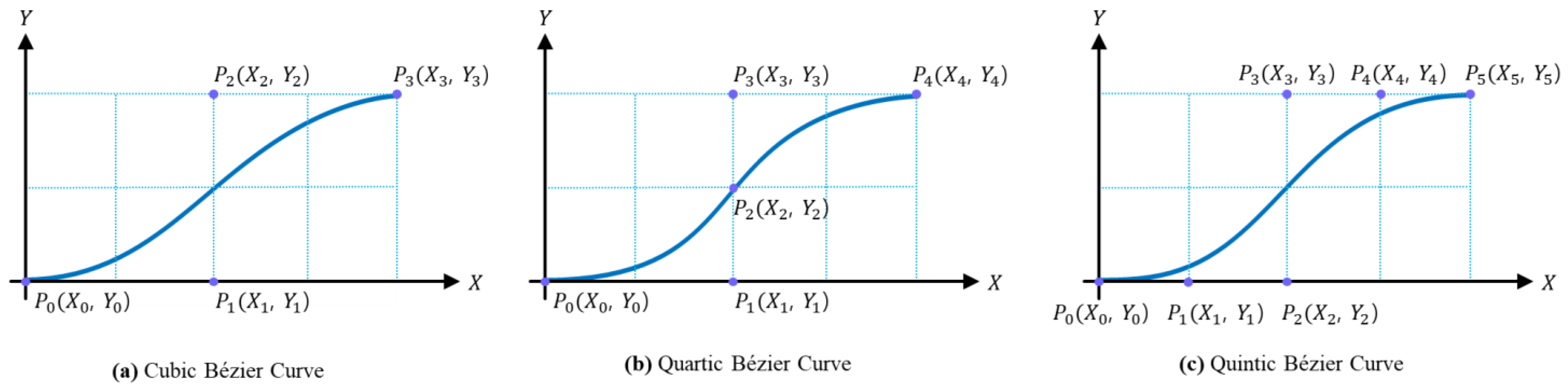
2.2. Bézier Curve Trajectory Generation
2.3. Autonomous Driving System Based on Vehicle Trajectory Prediction
3. Proposed Collision-Avoidance Path Planning Method
3.1. Overall Architecture of the Proposed Method
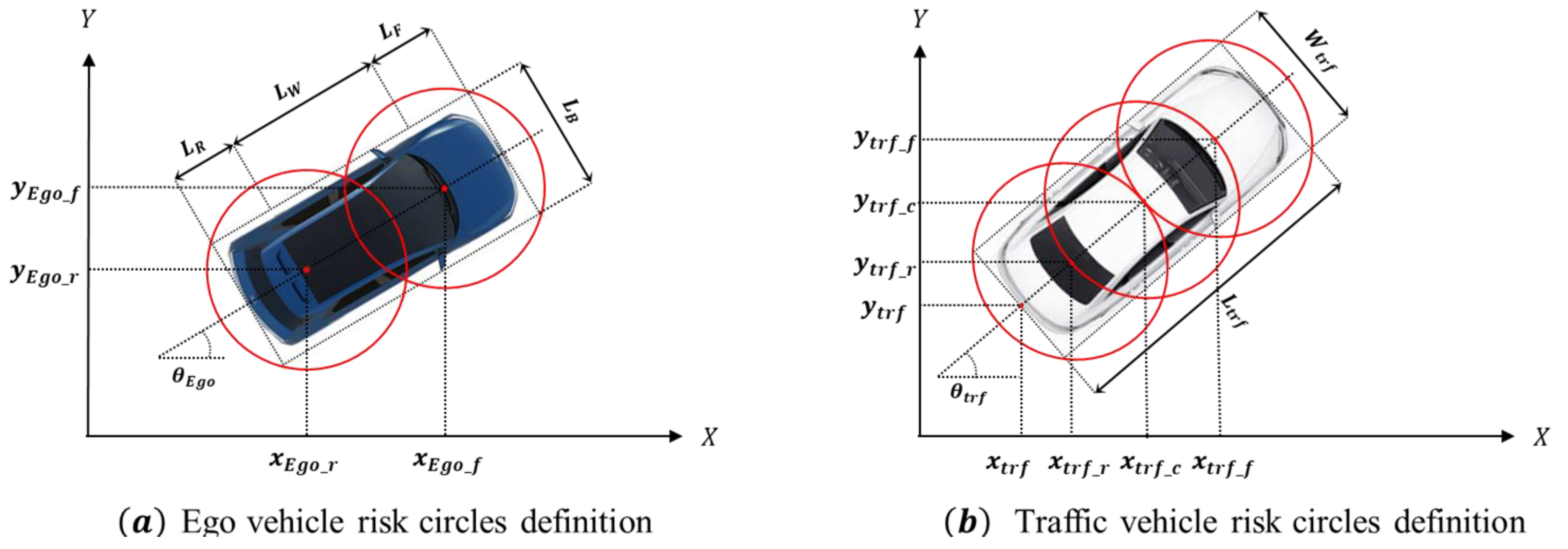
3.2. Risk Assessment
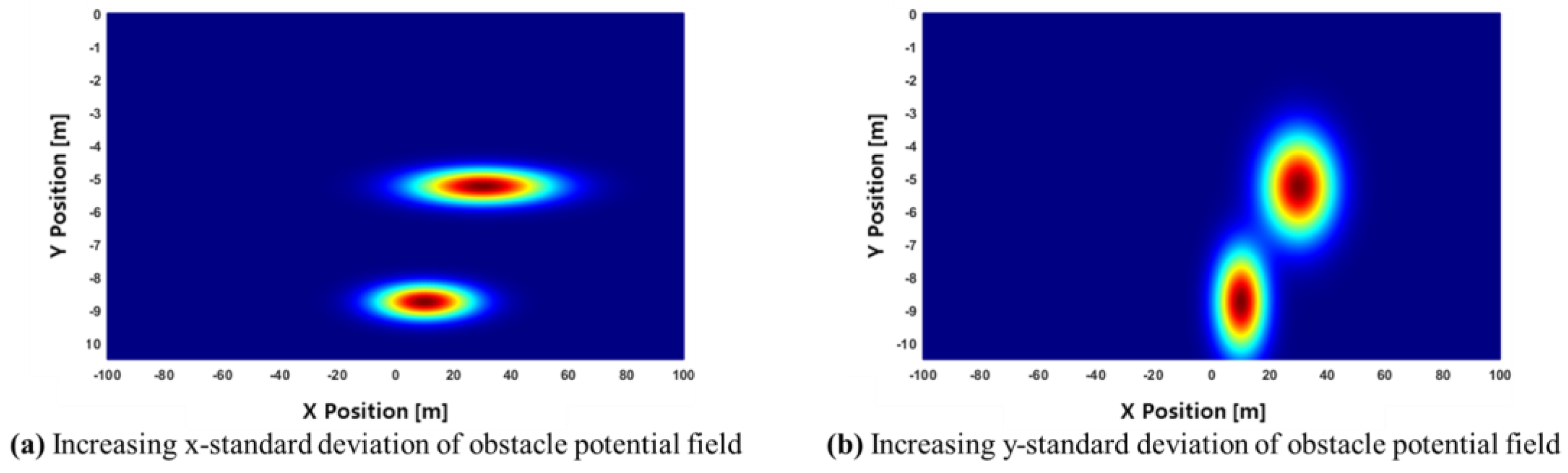
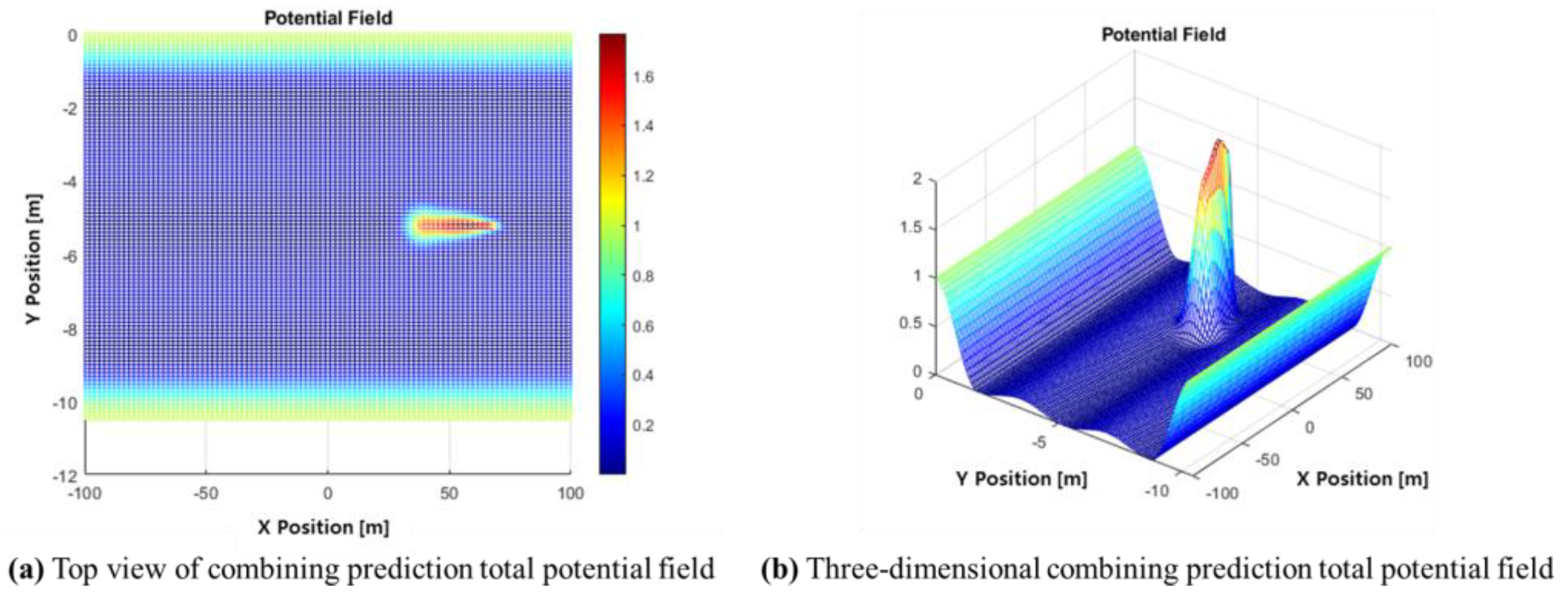
3.3. Artificial Potential Field with Prediction Information
3.4. Path Generation and Optimisation Based on the Bézier Curve
3.4.1. Quartic Bézier Curve Modeling
3.4.2. Quintic Bézier Curve Modeling
3.4.3. Path Optimization
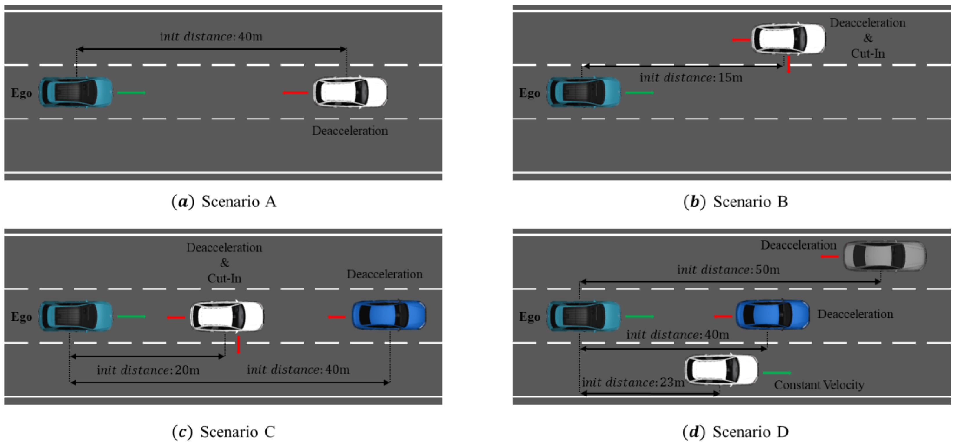
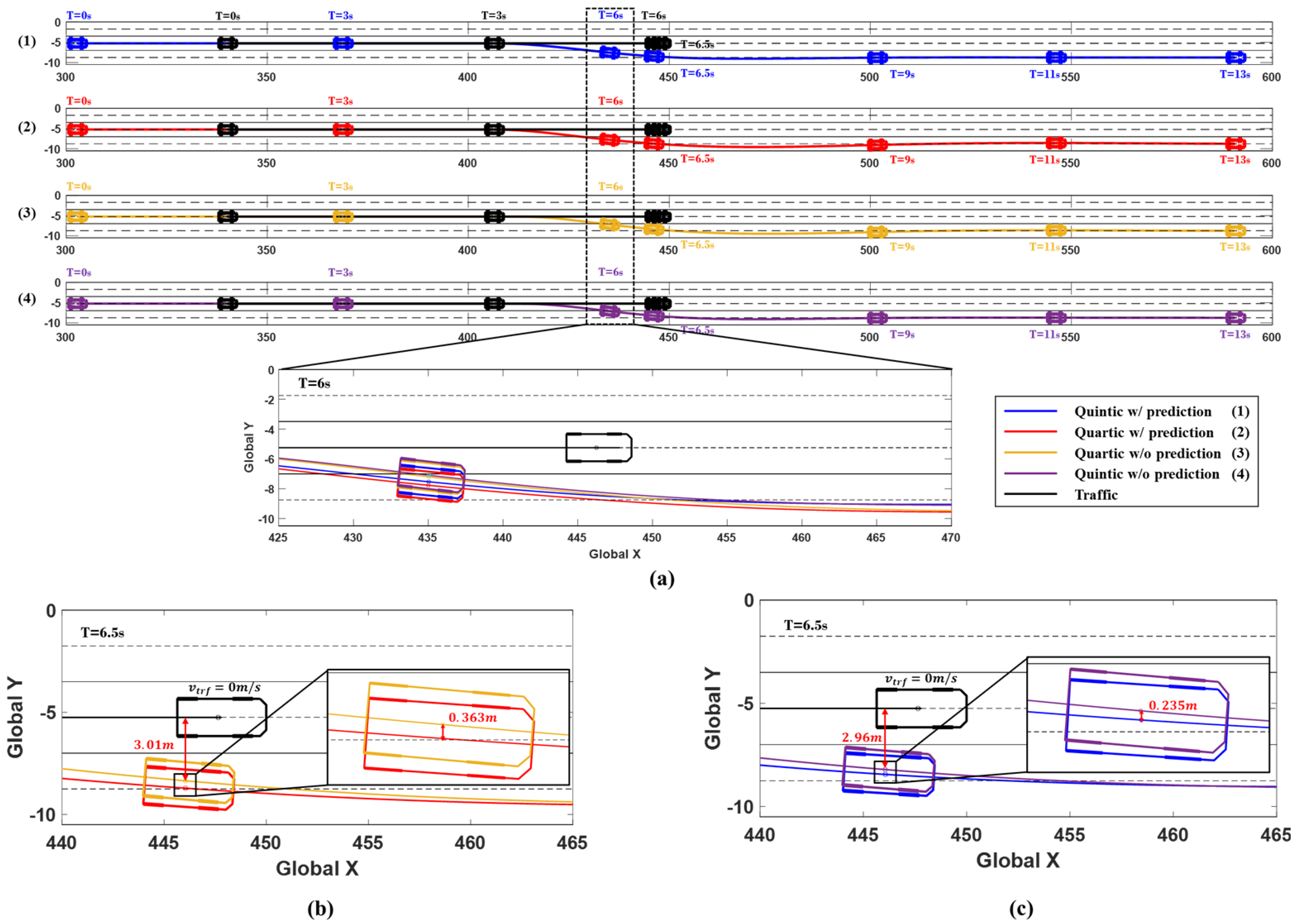
4. Simulation Results
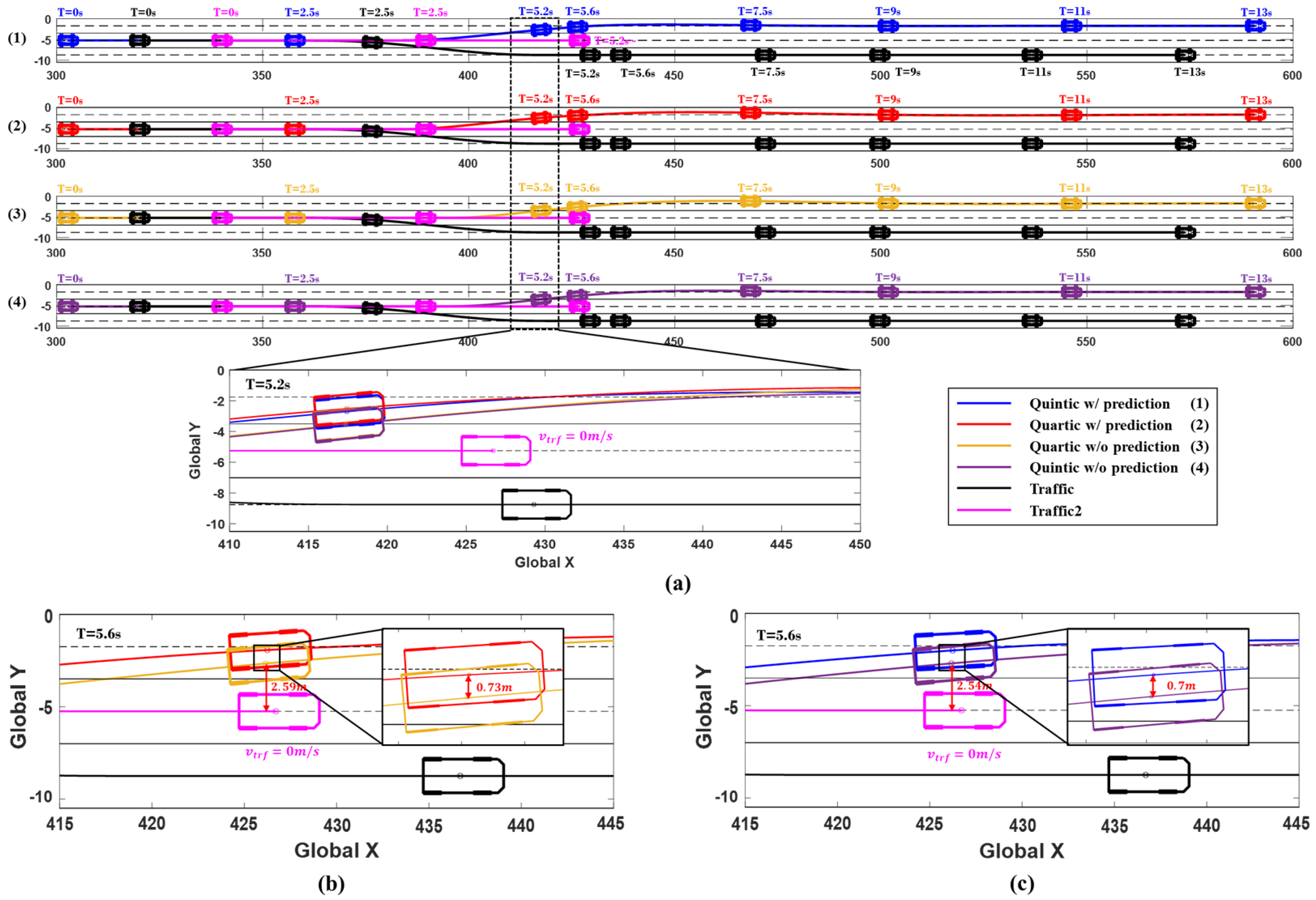
- Driving trajectory—to visualize the overall driving situation for each scenario.
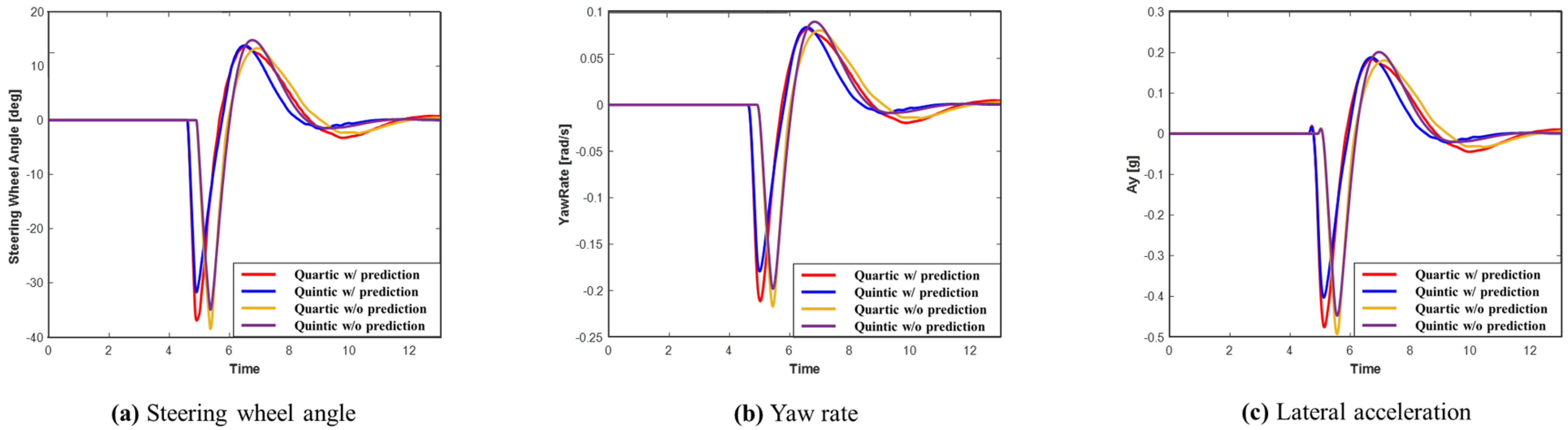
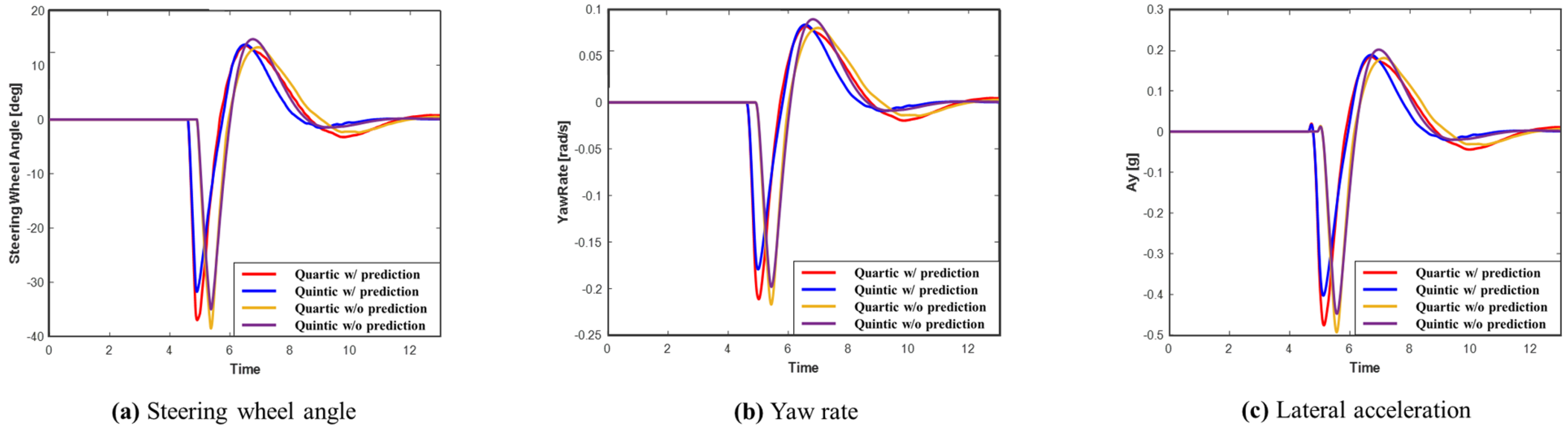
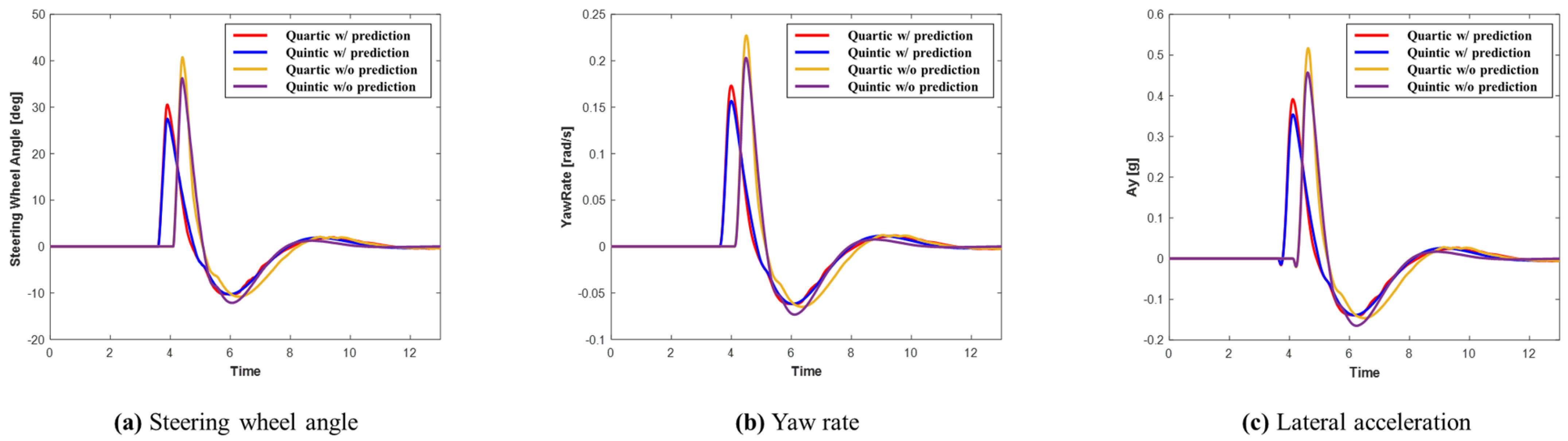
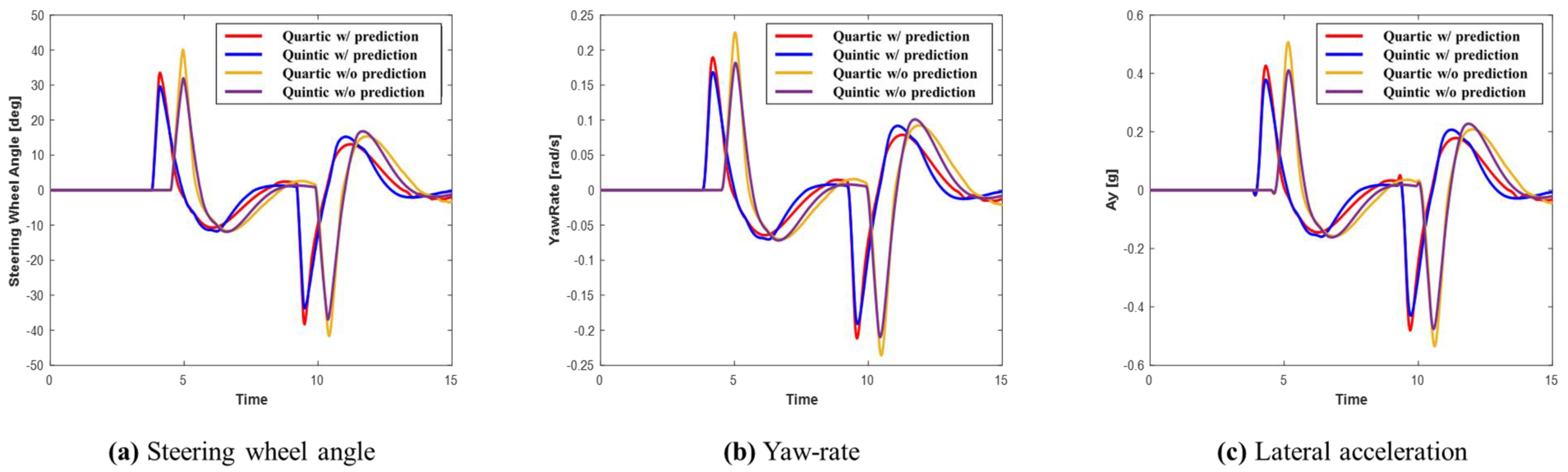
- Steering wheel angle, yaw rate, and lateral acceleration plots—to assess the vehicle’s lateral stability.
- Maximum value analysis—to examine the system’s lateral stability during the avoidance maneuver.
4.1. Simulation Scenario A
4.2. Simulation Scenario B
4.3. Simulation Scenario C
4.4. Simulation Scenario D
5. Conclusions
Author Contributions
Funding
Institutional Review Board Statement
Informed Consent Statement
Data Availability Statement
Conflicts of Interest
References
- Ma, Y.; Wang, Z.; Yang, H.; Yang, L. Artificial intelligence applications in the development of autonomous vehicles: A survey. IEEE/CAA J. Autom. Sin. 2020, 7, 315–329. [Google Scholar] [CrossRef]
- Schwarting, W.; Alonso-Mora, J.; Rus, D. Planning and decision-making for autonomous vehicles. Annu. Rev. Control. Robot. Auton. Syst. 2018, 1, 187–210. [Google Scholar] [CrossRef]
- Chan, C.-Y. Advancements, prospects, and impacts of automated driving systems. Int. J. Transp. Sci. Technol. 2017, 6, 208–216. [Google Scholar] [CrossRef]
- Chen, L.; Li, Y.; Huang, C.; Li, B.; Xing, Y.; Tian, D.; Li, L.; Hu, Z.; Na, X.; Li, Z.; et al. Milestones in autonomous driving and intelligent vehicles: Survey of surveys. IEEE Trans. Intell. Veh. 2023, 8, 1046–1056. [Google Scholar] [CrossRef]
- ISO 26262-10:2018; Road Vehicles—Functional Safety—Part 10: Guideline on ISO 26262. ISO: Geneva, Switzerland, 2018.
- ISO 39003-:2023; Road Traffic Safety—Guidance on Ethical Considerations Relating to Safety for Autonomous Vehicles. ISO: Geneva, Switzerland, 2023.
- Autonomous Vehicle Collision Reports. Available online: https://www.dmv.ca.gov/portal/vehicle-industry-services/autonomous-vehicles/autonomous-vehicle-collision-reports/ (accessed on 4 October 2024).
- Katrakazas, C.; Quddus, M.; Chen, W.-H.; Deka, L. Real-time motion planning methods for autonomous on-road driving: State-of-the-art and future research directions. Transp. Res. C 2015, 60, 416–442. [Google Scholar] [CrossRef]
- Favarò, F.M.; Nader, N.; Eurich, S.O.; Tripp, M.; Varadaraju, N. Examining accident reports involving autonomous vehicles in California. PLoS ONE 2017, 12, e0184952. [Google Scholar] [CrossRef]
- González, D.; Pérez, J.; Milanés, V.; Nashashibi, F. A review of motion planning techniques for automated vehicles. IEEE Trans. Intell. Transp. Syst. 2015, 17, 1135–1145. [Google Scholar] [CrossRef]
- Candela, E.; Feng, Y.; Mead, D.; Demiris, Y.; Angeloudis, P. Fast collision prediction for autonomous vehicles using a stochastic dynamics model. In Proceedings of the IEEE International Intelligent Transportation Systems Conference (ITSC), Indianapolis, IN, USA, 19–22 September 2021; Volume 2021, pp. 211–216. [Google Scholar]
- Huang, R.; Zhuo, G.; Xiong, L.; Lu, S.; Tian, W. A Review of Deep Learning-Based Vehicle Motion Prediction for Autonomous Driving. Sustainability 2023, 15, 14716. [Google Scholar] [CrossRef]
- Fang, L.; Jiang, Q.; Shi, J.; Zhou, B. TPNet: Trajectory Proposal Network for Motion Prediction. In Proceedings of the 2020 IEEE/CVF Conference on Computer Vision and Pattern Recognition (CVPR), Seattle, WA, USA, 13–19 June 2020; pp. 6796–6805. [Google Scholar]
- Polychronopoulos, A.; Tsogas, M.; Amditis, A.J.; Andreone, L. Sensor Fusion for Predicting Vehicles’ Path for Collision Avoidance Systems. IEEE Trans. Intell. Transp. Syst. 2007, 8, 549–562. [Google Scholar] [CrossRef]
- Da, F.; Zhang, Y. Path-Aware Graph Attention for HD Maps in Motion Prediction. In Proceedings of the International Conference on Robotics and Automation (ICRA), Philadelphia, PA, USA, 23–27 May 2022; pp. 6430–6436. [Google Scholar]
- Khatib, O. The Potential Field Approach and Operational Space Formulation in Robot Control, Adaptive and Learning Systems; Springer: Boston, MA, USA, 1986; pp. 367–377. [Google Scholar]
- Tran, H.N.; Shin, J.-H.; Jee, K.-S.; Moon, H.-G. Oscillation reduction for artificial potential field using vector projections for robotic manipulators. J. Mech. Sci. Technol. 2023, 37, 3273–3280. [Google Scholar] [CrossRef]
- Matoui, F.; Boussaid, B.; Abdelkrim, M.N. Local minimum solution for the potential field method in multiple robot motion planning task. In Proceedings of the 16th International Conference on Sciences and Techniques of Automatic Control and Computer Engineering (STA), Monastir, Tunisia, 21–23 December 2015; pp. 452–457. [Google Scholar]
- Rasekhipour, Y.; Khajepour, A.; Chen, S.-K.; Litkouhi, B. A potential field-based model predictive path-planning controller for autonomous road vehicles. IEEE Trans. Intell. Transp. Syst. 2017, 18, 1255–1267. [Google Scholar] [CrossRef]
- Wahid, N.; Zamzuri, H.; Amer, N.H.; Dwijotomo, A.; Saruchi, S.A.; Mazlan, S.A. Vehicle collision avoidance motion planning strategy using artificial potential field with adaptive multi-speed scheduler. IET Intell. Transp. Syst. 2020, 14, 1200–1209. [Google Scholar] [CrossRef]
- Ma, Q.; Li, M.; Huang, G.; Ullah, S. Overtaking Path Planning for CAV based on Improved Artificial Potential Field. IEEE Trans. Veh. Technol. 2023, 9, 1–13. [Google Scholar] [CrossRef]
- Huang, Y.; Ding, H.; Zhang, Y.; Wang, H.; Cao, D.; Xu, N.; Hu, C. A motion planning and tracking framework for autonomous vehicles based on artificial potential field elaborated resistance network approach. IEEE Trans. Ind. Electron. 2020, 67, 1376–1386. [Google Scholar] [CrossRef]
- Lin, P.; Choi, W.Y.; Ho Yang, J.H.; Chung, C.C. Waypoint tracking for collision avoidance using artificial potential field. In Proceedings of the 39th Chinese Control. Conference, Shenyang, China, 27–29 July 2020; Volume CCC, pp. 5455–5460. [Google Scholar]
- Shang, X.; Eskandarian, A. Emergency collision avoidance and mitigation using model predictive control and artificial potential function. IEEE Trans. Intell. Veh. 2023, 8, 3458–3472. [Google Scholar] [CrossRef]
- Choi, J.-W.; Curry, R.; Elkaim, G. Path Planning Based on Bézier Curve for Autonomous Ground Vehicles, Advances in Electrical and Electronics Engineering—IAENG; Special ed. of the World Congress on Engineering and Computer Science; IEEE: San Francisco, CA, USA, 2008; pp. 158–166. [Google Scholar]
- Han, L.; Yashiro, H.; Tehrani Nik Nejad, H.; Do, Q.H.; Mita, S. Bézier Curve Based Path Planning for Autonomous Vehicle in Urban Environment; IEEE Intelligent Vehicles Symposium: La Jolla, CA, USA, 2010; pp. 1036–1042. [Google Scholar]
- Li, H.; Luo, Y.; Wu, J. Collision-Free Path Planning for intelligent vehicles based on Bézier curve. IEEE Access 2019, 7, 123334–123340. [Google Scholar] [CrossRef]
- Chen, J.; Zhao, P.; Mei, T.; Liang, H. Lane change path planning based on piecewise Bézier curve for autonomous vehicle. In Proceedings of the 2013 IEEE International Conference on Vehicular Electronics and Safety, Dongguan, China, 28–30 July 2013; pp. 17–22. [Google Scholar]
- Moreau, J.; Melchior, P.; Victor, S.; Cassany, L.; Moze, M.; Aioun, F.; Guillemard, F. Reactive path planning in intersection for autonomous vehicle. IFAC PapersOnLine 2019, 52, 109–114. [Google Scholar] [CrossRef]
- Chen, C.; He, Y.; Bu, C.; Han, J.; Zhang, X. Quartic Bézier curve based trajectory generation for autonomous vehicles with curvature and velocity constraints. In Proceedings of the IEEE International Conference on Robotics and Automation (ICRA), Hong Kong, China, 31 May–7 June 2014; pp. 6108–6113. [Google Scholar]
- Zhang, L.; Xiao, W.; Zhang, Z.; Meng, D. Surrounding vehicles motion prediction for risk assessment and motion planning of autonomous vehicle in highway scenarios. IEEE Access 2020, 8, 209356–209376. [Google Scholar] [CrossRef]
- Yildirim, M.; Mozaffari, S.; McCutcheon, L.; Dianati, M.; Tamaddoni-Nezhad, A.; Fallah, S. Prediction based decision making for autonomous highway driving. In Proceedings of the IEEE 25th International Conference on Intelligent Transportation Systems (ITSC), Macau, China, 8–12 October 2022; Volume 2022, pp. 138–145. [Google Scholar]
- Yoon, Y.; Kim, C.; Lee, J.; Yi, K. Interaction-aware probabilistic trajectory prediction of cut-in vehicles using Gaussian process for proactive control of autonomous vehicles. IEEE Access 2021, 9, 63440–63455. [Google Scholar] [CrossRef]
- Wang, X.; Hu, J.; Wei, C.; Li, L.; Li, Y.; Du, M. A novel lane-change decision-making with long-time trajectory prediction for autonomous vehicle. IEEE Access 2023, 11, 137437–137449. [Google Scholar] [CrossRef]
- Meng, D.; Xiao, W.; Zhang, L.; Zhang, Z.; Liu, Z. Vehicle Trajectory Prediction based Predictive Collision Risk Assessment for Autonomous Driving in Highway Scenarios. arXiv 2023, arXiv:2304.05610. [Google Scholar]
- Kim, J.-H.; Kum, D.-S. Threat prediction algorithm based on local path candidates and surrounding vehicle trajectory predictions for automated driving vehicles. In Proceedings of the IEEE Intelligent Vehicles Symposium, Seoul, Republic of Korea, 28 June–1 July 2015; Volume IV, pp. 1220–1225. [Google Scholar]
- Kang, T.W.; Yang, J.H.; Choi, W.Y.; Chung, C.C. Time Headway for Overtaking Control of Autonomous Driving Vehicle. In Proceedings of the KSAE Spring Conference, Proceedings, Pyeongchang, Republic of Korea, 22 May 2019; pp. 810–815. [Google Scholar]
- Yimer, T.H.; Wen, C.; Yu, X.; Jiang, C. A Study of the Minimum Safe Distance Between Human Driven and Driverless Cars Using Safe Distance Model. arXiv 2020, arXiv:2006.07022. [Google Scholar]
- Tang, X.; Yan, Y.; Wang, B. Trajectory tracking control of autonomous vehicles combining ACT-R cognitive framework and preview tracking theory. IEEE Access 2023, 11, 137067–137082. [Google Scholar] [CrossRef]
- Tyagi, I. Threat Assessment for avoiding collsions with perpendicular vehicles at Intersections. In Proceedings of the IEEE International Conference on Electro Information Technology (EIT), Mt. Pleasant, MI, USA, 14–15 May 2021; Volume 2021, pp. 184–187. [Google Scholar]
- Diachuk, M.; Easa, S.M. Motion planning for autonomous vehicles based on sequential optimization. Vehicles 2022, 4, 344–374. [Google Scholar] [CrossRef]
- Li, B.; Acarman, T.; Zhang, Y.; Ouyang, Y.; Yaman, C.; Kong, Q.; Zhong, X.; Peng, X. Optimization-based trajectory planning for autonomous parking with irregularly placed obstacles: A lightweight iterative framework. IEEE Trans. Intell. Transp. Syst. 2022, 23, 11970–11981. [Google Scholar] [CrossRef]
- Jiang, Y.; Liu, Z.; Qian, D.; Zuo, H.; He, W.; Wang, J. Robust online path planning for autonomous vehicle using sequential quadratic programming. In Proceedings of the IEEE Intelligent Vehicles Symposium, Aachen, Germany, 4–9 June 2022; Volume IV, pp. 175–182. [Google Scholar]
- Wei, Y.; Xu, H. Path planning of autonomous driving based on quadratic. In Proceedings of the Optimization 9th International Conference on Control, Automation and Robotics (ICCAR), Beijing, China, 21–23 April 2023; Volume 2023, pp. 308–312. [Google Scholar]
- ISO 34502-:2022; Road Vehicles—Test Scenarios for Automated Driving Systems—Scenario Based Safety Evaluation Framework. ISO: Geneva, Switzerland, 2022.


| Unit | ||||||
|---|---|---|---|---|---|---|
| 0.845 | 2.97 | 0.82 | 1.89 | 4.47 | 1.97 | m |
| Symbol | Description | Value | Unit |
|---|---|---|---|
| Width of each lane | 3.5 | m | |
| Global lateral position of the first lane | −1.75 | m | |
| Global lateral position of the third lane | −8.75 | m | |
| Parameter for the road potential field function | 0.1 | -- | |
| Longitudinal deviation for obstacle potential field | 5 | -- | |
| Lateral deviation for obstacle potential field | 0.5 | -- | |
| μ | Parameter to prevent errors in the obstacle potential field | 1 × 10⁻⁵ | -- |
| Symbol | Description | Value | Unit |
|---|---|---|---|
| Coefficient of curvature term for objective function | 1 | -- | |
| Coefficient of total potential value term for objective function | 1 | -- | |
| Coefficient of jerk term for objective function | 1 | -- | |
| Maximum curvature | 0.3 | ||
| Threshold of TTC | 2 | s | |
| Coefficient of the laterally offset term for objective function | 5 | -- |
| Scenario A | Maximum Lateral Acceleration (g) | Maximum Yaw Rate (deg/s) | Maximum Steering Wheel Angle (deg) |
|---|---|---|---|
| Quartic w/prediction | 0.4758 | 0.2114 | 36.9478 |
| Quintic w/prediction | 0.4030 | 0.1794 | 31.7464 |
| Quartic w/o prediction | 0.5510 | 0.2449 | 44.6391 |
| Quintic w/o prediction | 0.5008 | 0.2222 | 39.9116 |
| Scenario B | Maximum Lateral Acceleration (g) | Maximum Yaw Rate (deg/s) | Maximum Steering Wheel Angle (deg) |
|---|---|---|---|
| Quartic w/prediction | 0.4716 | 0.2090 | 37.2937 |
| Quintic w/prediction | 0.4213 | 0.1865 | 33.0276 |
| Quartic w/o prediction | 0.5574 | 0.2429 | 44.6627 |
| Quintic w/o prediction | 0.5054 | 0.2247 | 40.1564 |
| Scenario C | Maximum Lateral Acceleration (g) | Maximum Yaw Rate (deg/s) | Maximum Steering Wheel Angle (deg) |
|---|---|---|---|
| Quartic w/prediction | 0.3914 | 0.1731 | 30.5570 |
| Quintic w/prediction | 0.3539 | 0.1566 | 27.4941 |
| Quartic w/o prediction | 0.5169 | 0.2271 | 40.7668 |
| Quintic w/o prediction | 0.4570 | 0.2030 | 36.2411 |
| Scenario D | Maximum Lateral Acceleration (g) | Maximum Yaw Rate (deg/s) | Maximum Steering Wheel Angle (deg) |
|---|---|---|---|
| Quartic w/prediction | 0.4802 | 0.2115 | 38.2716 |
| Quintic w/prediction | 0.4300 | 0.1908 | 33.7257 |
| Quartic w/o prediction | 0.5956 | 0.2601 | 46.2612 |
| Quintic w/o prediction | 0.5242 | 0.2327 | 41.6060 |
Disclaimer/Publisher’s Note: The statements, opinions and data contained in all publications are solely those of the individual author(s) and contributor(s) and not of MDPI and/or the editor(s). MDPI and/or the editor(s) disclaim responsibility for any injury to people or property resulting from any ideas, methods, instructions or products referred to in the content. |
© 2024 by the authors. Licensee MDPI, Basel, Switzerland. This article is an open access article distributed under the terms and conditions of the Creative Commons Attribution (CC BY) license (https://creativecommons.org/licenses/by/4.0/).
Share and Cite
Ahn, S.; Oh, T.; Yoo, J. Collision Avoidance Path Planning for Automated Vehicles Using Prediction Information and Artificial Potential Field. Sensors 2024, 24, 7292. https://doi.org/10.3390/s24227292
Ahn S, Oh T, Yoo J. Collision Avoidance Path Planning for Automated Vehicles Using Prediction Information and Artificial Potential Field. Sensors. 2024; 24(22):7292. https://doi.org/10.3390/s24227292
Chicago/Turabian StyleAhn, Sumin, Taeyoung Oh, and Jinwoo Yoo. 2024. "Collision Avoidance Path Planning for Automated Vehicles Using Prediction Information and Artificial Potential Field" Sensors 24, no. 22: 7292. https://doi.org/10.3390/s24227292
APA StyleAhn, S., Oh, T., & Yoo, J. (2024). Collision Avoidance Path Planning for Automated Vehicles Using Prediction Information and Artificial Potential Field. Sensors, 24(22), 7292. https://doi.org/10.3390/s24227292