

Colorful Image Colorization with Classification and Asymmetric Feature Fusion


Abstract
1. Introduction
- A category conversion module and a category balance module are proposed to significantly reduce the training time.
- A classification subnetwork is proposed to improve colorization accuracy and saturation.
- An AFF module is introduced to prevent color overflow and to improve the colorization effect.
2. Related Work
2.1. Traditional Colorization Method
2.1.1. Color Expansion
2.1.2. Color Transfer
2.2. Deep Learning-Based Colorization Algorithms
2.2.1. Regression Loss Function
2.2.2. Classification Loss Function
3. Method
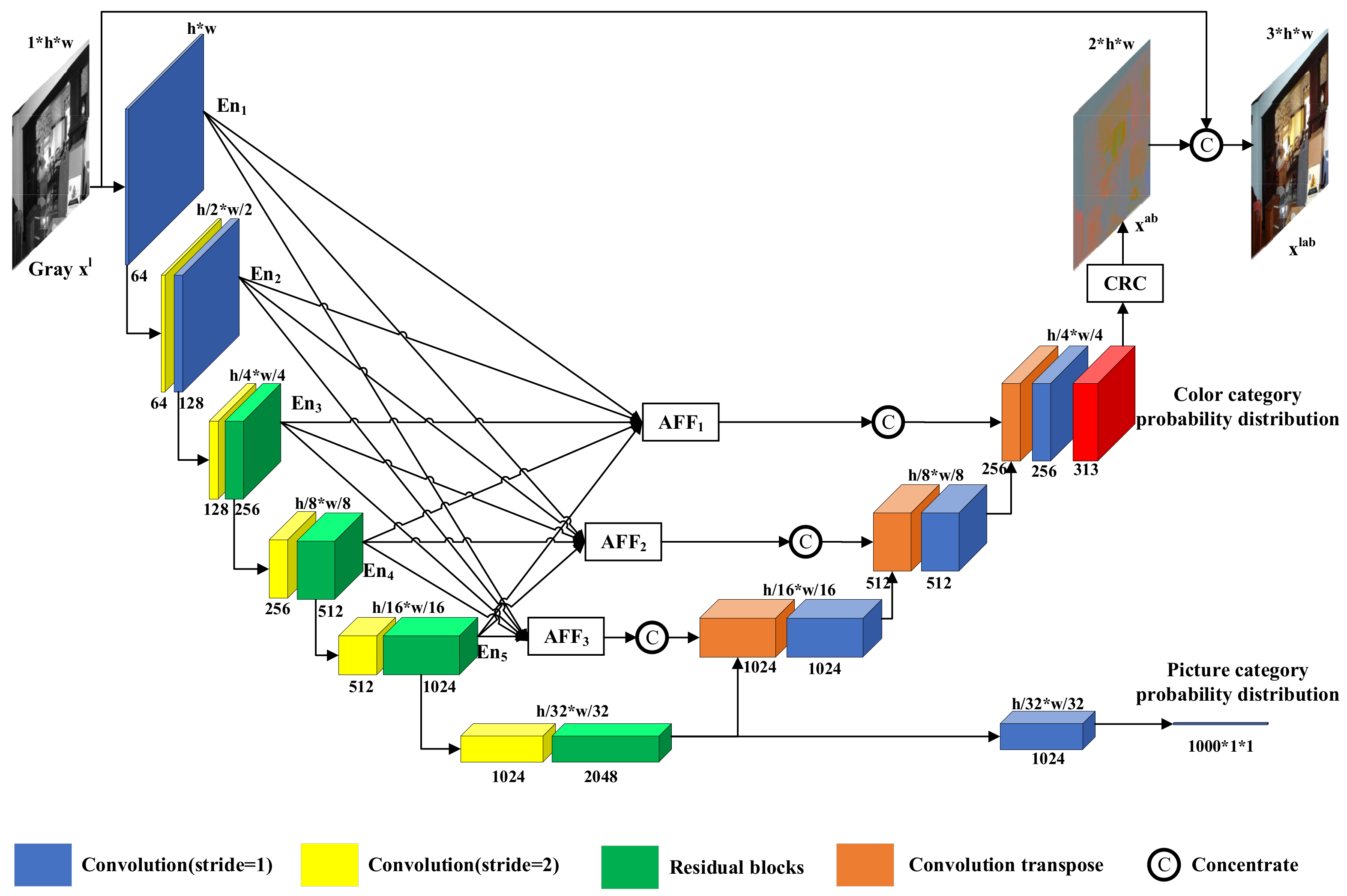
3.1. Overview
3.2. Calculating Color Categories and Balance Weights
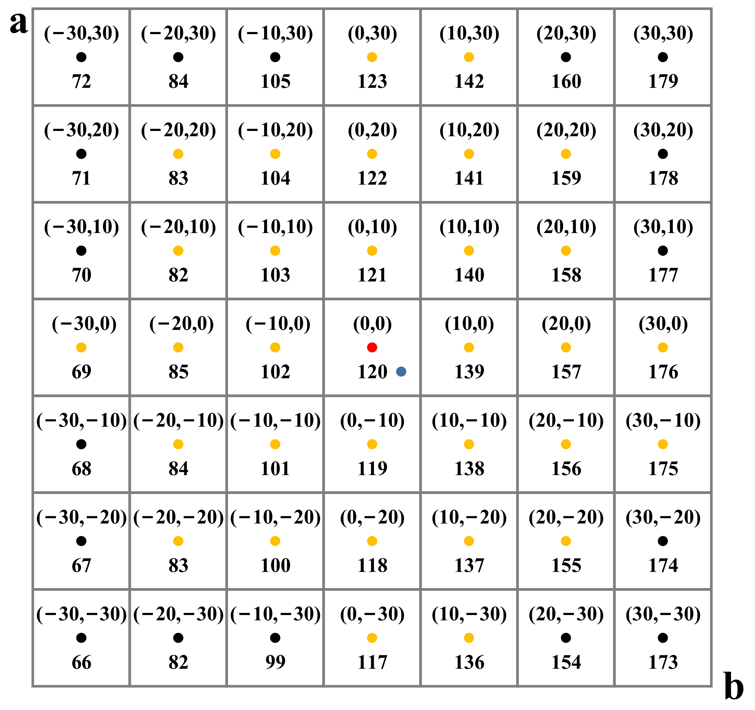
3.2.1. Category Conversion Module
3.2.2. Category Balance Module
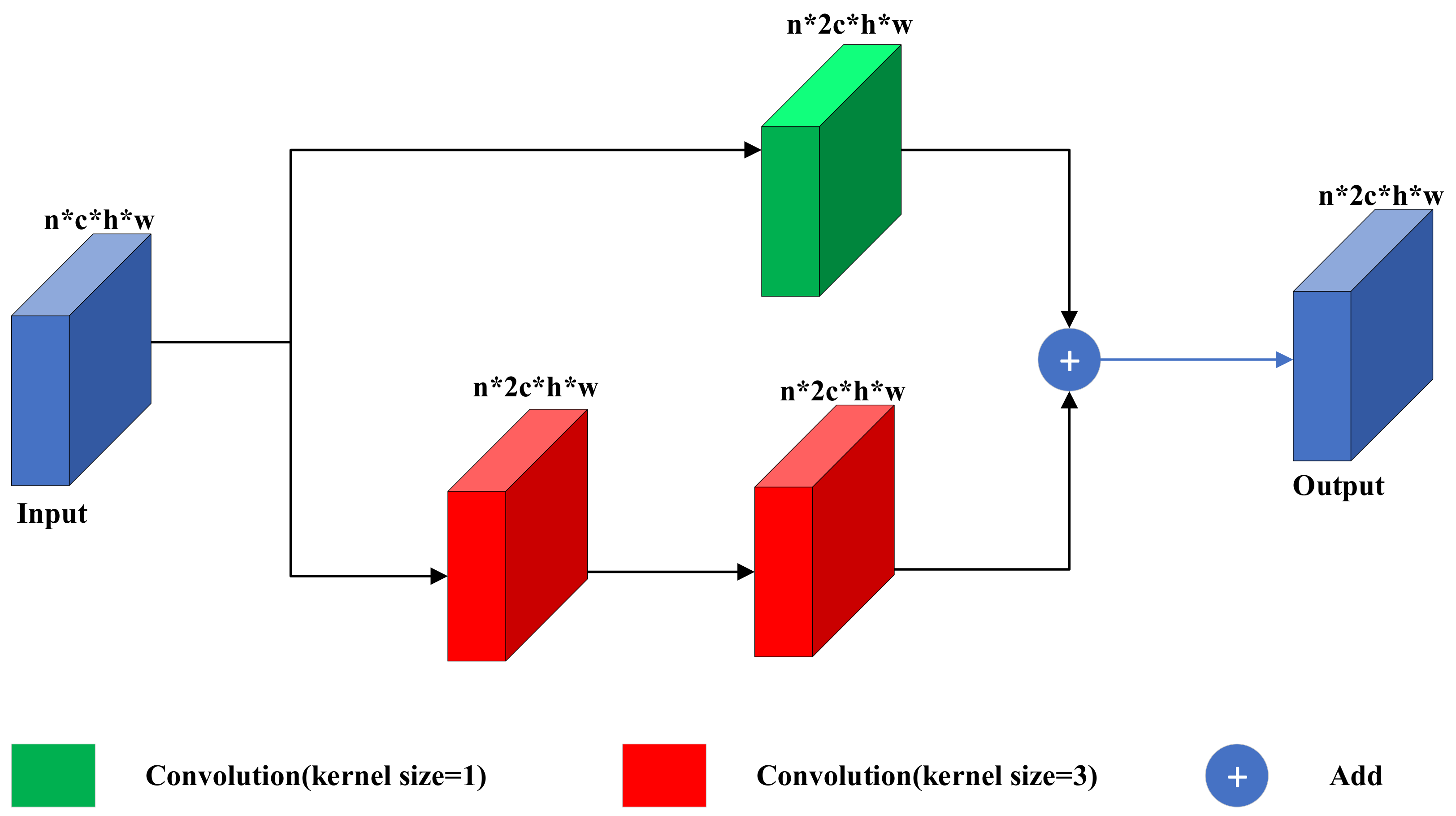
3.3. Residual Block
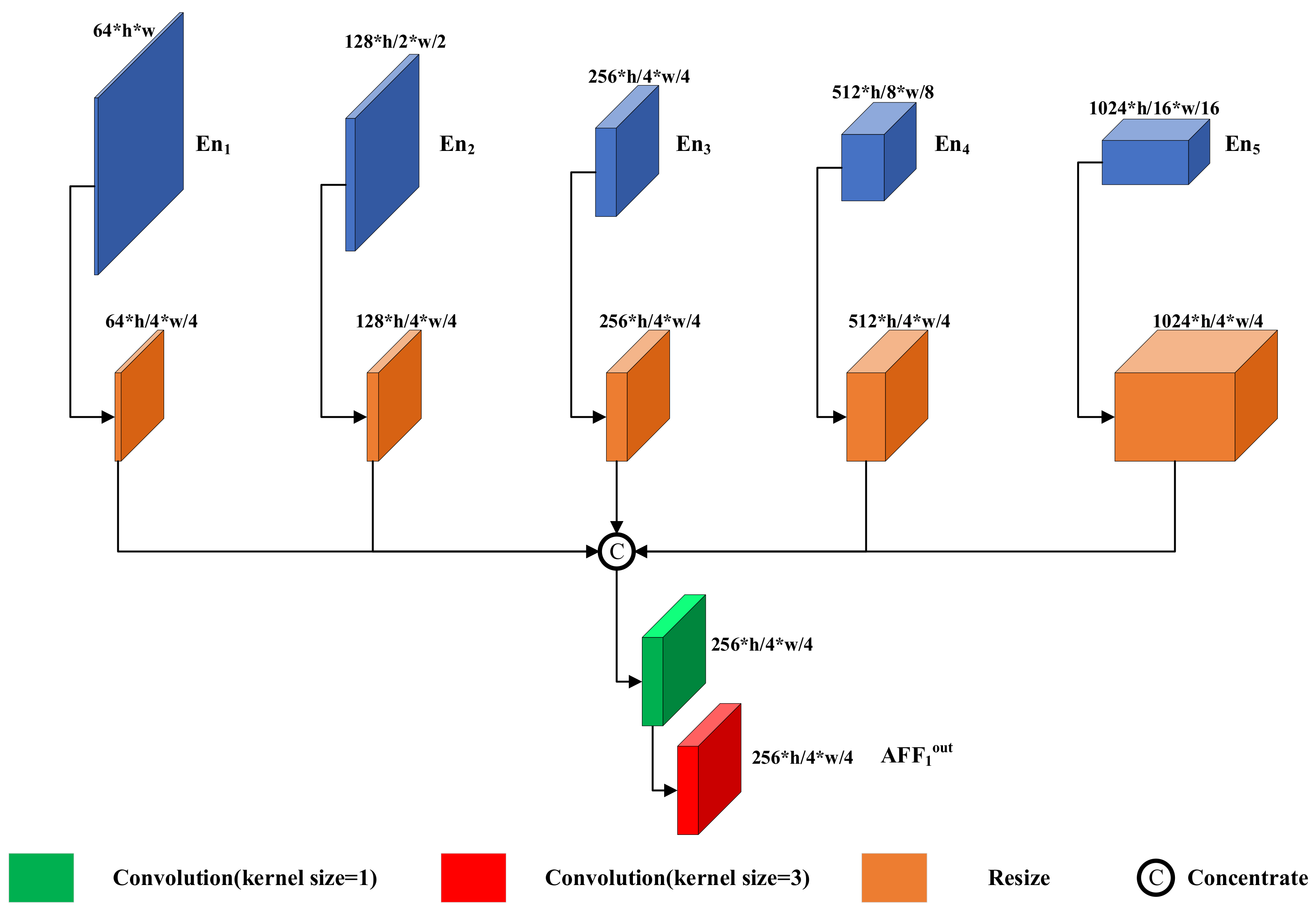
3.4. Asymmetric Feature Fusion Module
3.5. Color Recovery Module
3.6. Colorization with Classification
4. Experiments
4.1. Experimental Details
4.2. Calculating Time Experiments
4.3. Quantitative Analysis
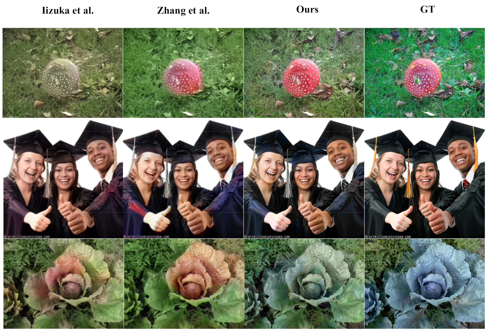
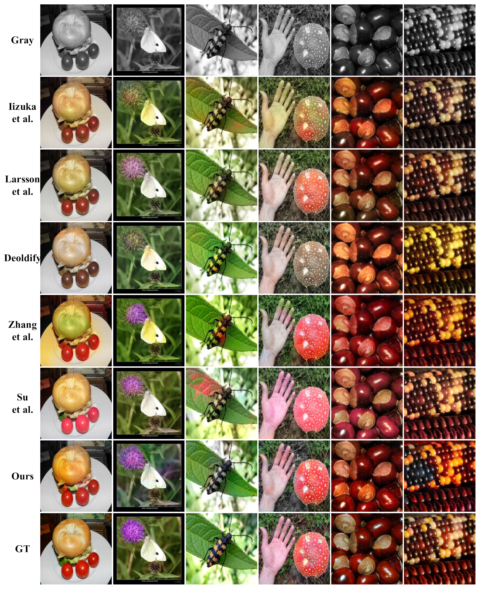
4.4. Qualitative Analysis
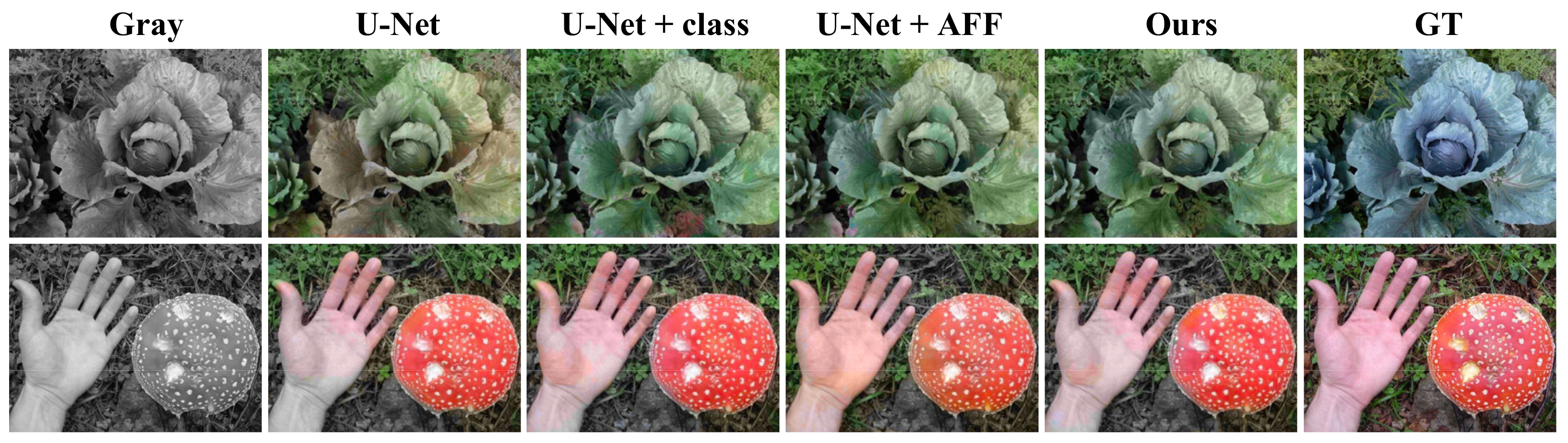
4.5. Ablation Experiments
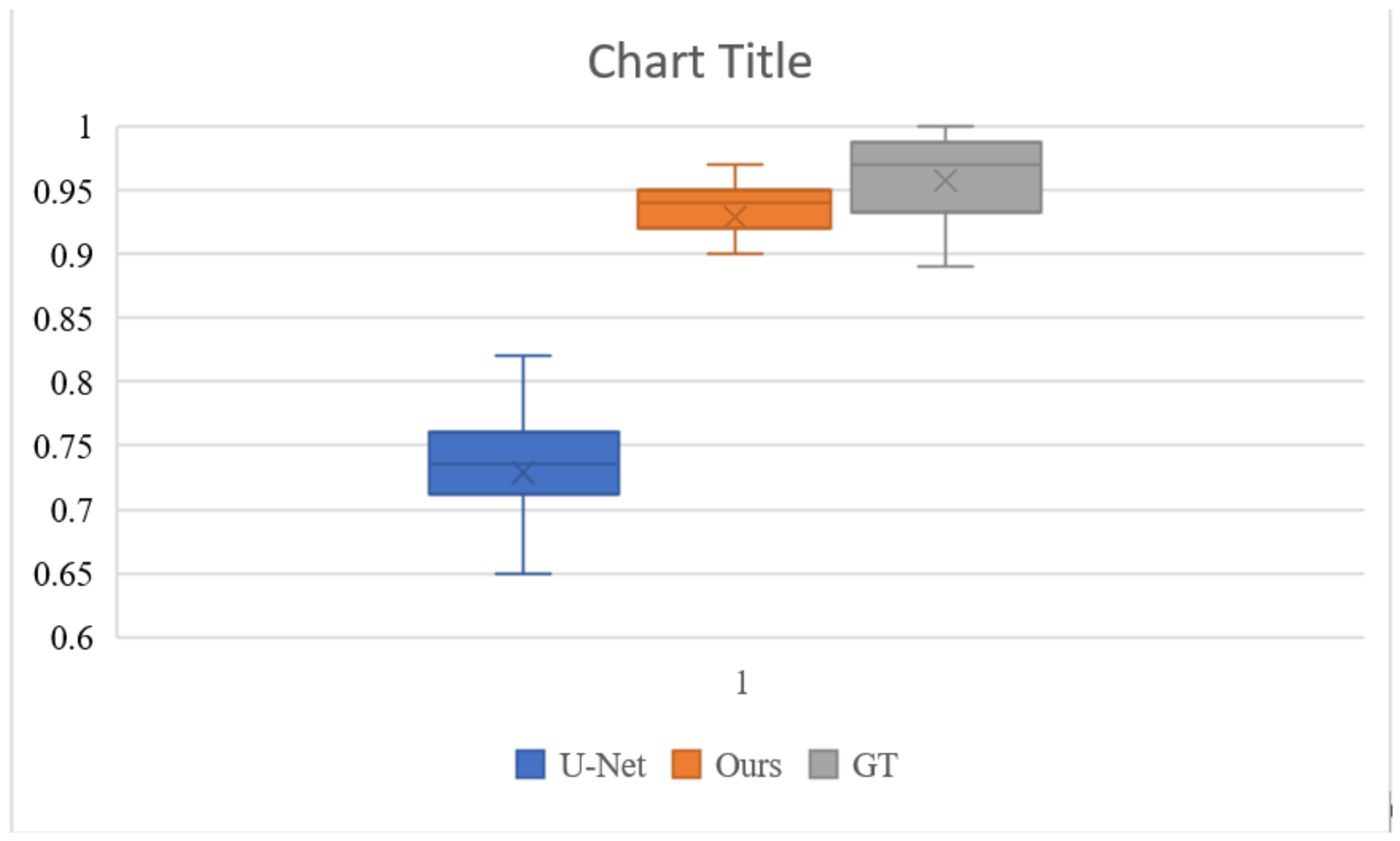
4.6. User Study
4.7. Limitation
5. Conclusions
Author Contributions
Funding
Institutional Review Board Statement
Informed Consent Statement
Data Availability Statement
Conflicts of Interest
References
- Levin, A.; Lischinski, D.; Weiss, Y. Colorization using optimization. ACM Trans. Graph. 2004, 23, 689–694. [Google Scholar] [CrossRef]
- Yatziv, L.; Sapiro, G. Fast image and video colorization using chrominance blending. IEEE Trans. Image Process. 2006, 15, 1120–1129. [Google Scholar] [CrossRef]
- Qu, Y.; Wong, T.-T.; Heng, P.-A. Manga Colorization. ACM Trans. Graph. 2006, 25, 1214–1220. [Google Scholar] [CrossRef]
- Luan, Q.; Wen, F.; Cohen-Or, D.; Liang, L.; Xu, Y.-Q.; Shum, H.-Y. Natural Image Colorization. In Proceedings of the 18th Eurographics Conference on Rendering Techniques, Grenoble, France, 25 June 2007; pp. 309–320. [Google Scholar]
- Welsh, T.; Ashikhmin, M.; Mueller, K. Transferring color to greyscale images. ACM Trans. Graph. 2002, 21, 277–280. [Google Scholar] [CrossRef]
- Irony, R.; Cohen-Or, D.; Lischinski, D. Colorization by Example. In Proceedings of the Eurographics Symposium on Rendering (2005), Konstanz, Germany, 29 June–1 July 2005; Bala, K., Dutre, P., Eds.; The Eurographics Association: Vienna, Austria, 2005. [Google Scholar]
- Liu, X.; Wan, L.; Qu, Y.; Wong, T.-T.; Lin, S.; Leung, C.-S.; Heng, P.-A. Intrinsic Colorization. In Proceedings of the ACM SIGGRAPH Asia 2008, New York, NY, USA, 1 December 2008. [Google Scholar]
- Wang, X.; Jia, J.; Liao, H.; Cai, L. Affective Image Colorization. J. Comput. Sci. Technol. 2012, 27, 1119–1128. [Google Scholar] [CrossRef]
- Cheng, Z.; Yang, Q.; Sheng, B. Deep Colorization. In Proceedings of the 2015 IEEE International Conference on Computer Vision (ICCV), Santiago, Chile, 7–13 December 2015; pp. 415–423. [Google Scholar]
- Larsson, G.; Maire, M.; Shakhnarovich, G. Learning Representations for Automatic Colorization. In Lecture Notes in Computer Science; Leibe, B., Matas, J., Sebe, N., Welling, M., Eds.; Springer: Cham, Switzerland, 2016; Volume 9908. [Google Scholar] [CrossRef]
- Iizuka, S.; Simo-Serra, E.; Ishikawa, H. Let there be color!: Joint end-to-end learning of global and local image priors for automatic image colorization with simultaneous classification. ACM Trans. Graph. 2016, 35, 1–11. [Google Scholar] [CrossRef]
- Nazeri, K.; Ng, E.; Ebrahimi, M. Image Colorization Using Generative Adversarial Networks. In International Conference on Articulated Motion and Deformable Objects; Springer: Berlin/Heidelberg, Germany, 2018; Volume 10945, pp. 85–94. [Google Scholar] [CrossRef]
- Isola, P.; Zhu, J.-Y.; Zhou, T.; Efros, A.A. Image-to-Image Translation with Conditional Adversarial Networks. In Proceedings of the IEEE Conference on Computer Vision and Pattern Recognition, Honolulu, HI, USA, 21–26 July 2017; pp. 1125–1134. [Google Scholar]
- Cao, Y.; Zhou, Z.; Zhang, W.; Yu, Y. Unsupervised Diverse Colorization via Generative Adversarial Networks. In Joint European Conference on Machine Learning and Knowledge Discovery in Databases; Springer: Berlin/Heidelberg, Germany, 2017; pp. 151–166. [Google Scholar] [CrossRef]
- Vitoria, P.; Raad, L.; Ballester, C. ChromaGAN: Adversarial Picture Colorization with Semantic Class Distribution. In Proceedings of the 2020 IEEE Winter Conference on Applications of Computer Vision (WACV), Snowmass Village, CO, USA, 1–5 March 2020; IEEE: New York, NY, USA, 2020; pp. 2434–2443. [Google Scholar]
- Zhang, R.; Zhu, J.-Y.; Isola, P.; Geng, X.; Lin, A.S.; Yu, T.; Efros, A.A. Real-time user-guided image colorization with learned deep priors. ACM Trans. Graph. 2017, 36, 1–11. [Google Scholar] [CrossRef]
- Zhao, J.; Han, J.; Shao, L.; Snoek, C.G.M. Pixelated Semantic Colorization. Int. J. Comput. Vis. 2019, 128, 818–834. [Google Scholar] [CrossRef]
- Antic, J. Jantic/Deoldify: A Deep Learning Based Project for Colorizing and Restoring Old Images (and Video!). Available online: https://github.com/jantic (accessed on 16 October 2019).
- Su, J.-W.; Chu, H.-K.; Huang, J.-B. Instance-Aware Image Colorization. In Proceedings of the IEEE/CVF Conference on Computer Vision and Pattern Recognition, Seattle, WA, USA, 13–19 June 2020; pp. 7965–7974. [Google Scholar] [CrossRef]
- Wu, Y.; Wang, X.; Li, Y.; Zhang, H.; Zhao, X.; Shan, Y. Towards Vivid and Diverse Image Colorization with Generative Color Prior. In Proceedings of the IEEE/CVF International Conference on Computer Vision, Montreal, QC, Canada, 10–17 October 2021; pp. 14377–14386. [Google Scholar] [CrossRef]
- Jin, X.; Li, Z.; Liu, K.; Zou, D.; Li, X.; Zhu, X.; Zhou, Z.; Sun, Q.; Liu, Q. Focusing on Persons: Colorizing Old Images Learning from Modern Historical Movies. In Proceedings of the 29th ACM International Conference on Multimedia, Virtual Event, 20–24 October 2021; pp. 1176–1184. [Google Scholar]
- Zhang, R.; Isola, P.; Efros, A.A. Colorful Image Colorization. In European Conference on Computer Vision; Springer: Berlin/Heidelberg, Germany, 2016; pp. 649–666. [Google Scholar]
- Ronneberger, O.; Fischer, P.; Brox, T. U-Net: Convolutional networks for biomedical image segmentation. In Medical Image Computing and Computer-Assisted Intervention 2015; Navab, N., Hornegger, J., Wells, W.M., Frangi, A.F., Eds.; Springer International Publishing: Cham, Switzerland, 2015; pp. 234–241. [Google Scholar] [CrossRef]
- Cho, S.-J.; Ji, S.-W.; Hong, J.-P.; Jung, S.-W.; Ko, S.-J. Rethinking Coarse-to-Fine Approach in Single Image Deblurring. In Proceedings of the IEEE/CVF International Conference on Computer Vision, Montreal, QC, Canada, 10–17 October 2021; pp. 4621–4630. [Google Scholar] [CrossRef]
- He, K.; Zhang, X.; Ren, S.; Sun, J. Deep residual learning for image recognition. In Proceedings of the 2016 IEEE Conference on Computer Vision and Pattern Recognition (CVPR), Las Vegas, NV, USA, 27–30 June 2016; pp. 770–778. [Google Scholar] [CrossRef]
- Kim, S.-W.; Kook, H.-K.; Sun, J.-Y.; Kang, M.-C.; Ko, S.-J. Parallel Feature Pyramid Network for Object Detection. In Computer Vision–ECCV 2018; Lecture Notes in Computer Science; Ferrari, V., Hebert, M., Sminchisescu, C., Weiss, Y., Eds.; Springer International Publishing: New York, NY, USA, 2018; Volume 11209, pp. 239–256. ISBN 978-3-030-01227-4. [Google Scholar]


| Methods | 43.9 Billion Pixels | 3.2 Million Pixels |
|---|---|---|
| Zhang et al. [22] | 3 days | 18.86 s |
| Ours | 2 h | 0.4 s |
| Method | PSNR↑ | SSIM↑ |
|---|---|---|
| Iizuka et al. [11] | 23.6362 | 0.9173 |
| Larsson et al. [10] | 25.1067 | 0.9266 |
| Deoldify [18] | 23.5372 | 0.9144 |
| Zhang et al. [22] | 21.7910 | 0.8915 |
| Su et al. [19] | 25.7440 | 0.9202 |
| Ours | 25.8803 | 0.9368 |
| Method | PSNR↑ | SSIM↑ |
|---|---|---|
| U-Net | 23.1783 | 0.8921 |
| U-Net + Classifier | 24.1615 | 0.9119 |
| U-Net + AFF | 24.7595 | 0.9260 |
| Ours | 25.8803 | 0.9368 |
| Approach | Naturalness (Median) |
|---|---|
| U-Net | 72.9% |
| Ours | 92.9% |
| GT | 95.8% |
Publisher’s Note: MDPI stays neutral with regard to jurisdictional claims in published maps and institutional affiliations. |
© 2022 by the authors. Licensee MDPI, Basel, Switzerland. This article is an open access article distributed under the terms and conditions of the Creative Commons Attribution (CC BY) license (https://creativecommons.org/licenses/by/4.0/).
Share and Cite
Wang, Z.; Yu, Y.; Li, D.; Wan, Y.; Li, M. Colorful Image Colorization with Classification and Asymmetric Feature Fusion. Sensors 2022, 22, 8010. https://doi.org/10.3390/s22208010
Wang Z, Yu Y, Li D, Wan Y, Li M. Colorful Image Colorization with Classification and Asymmetric Feature Fusion. Sensors. 2022; 22(20):8010. https://doi.org/10.3390/s22208010
Chicago/Turabian StyleWang, Zhiyuan, Yi Yu, Daqun Li, Yuanyuan Wan, and Mingyang Li. 2022. "Colorful Image Colorization with Classification and Asymmetric Feature Fusion" Sensors 22, no. 20: 8010. https://doi.org/10.3390/s22208010
APA StyleWang, Z., Yu, Y., Li, D., Wan, Y., & Li, M. (2022). Colorful Image Colorization with Classification and Asymmetric Feature Fusion. Sensors, 22(20), 8010. https://doi.org/10.3390/s22208010