
Low SNR Multi-Emitter Signal Sorting and Recognition Method Based on Low-Order Cyclic Statistics CWD Time-Frequency Images and the YOLOv5 Deep Learning Model


Abstract
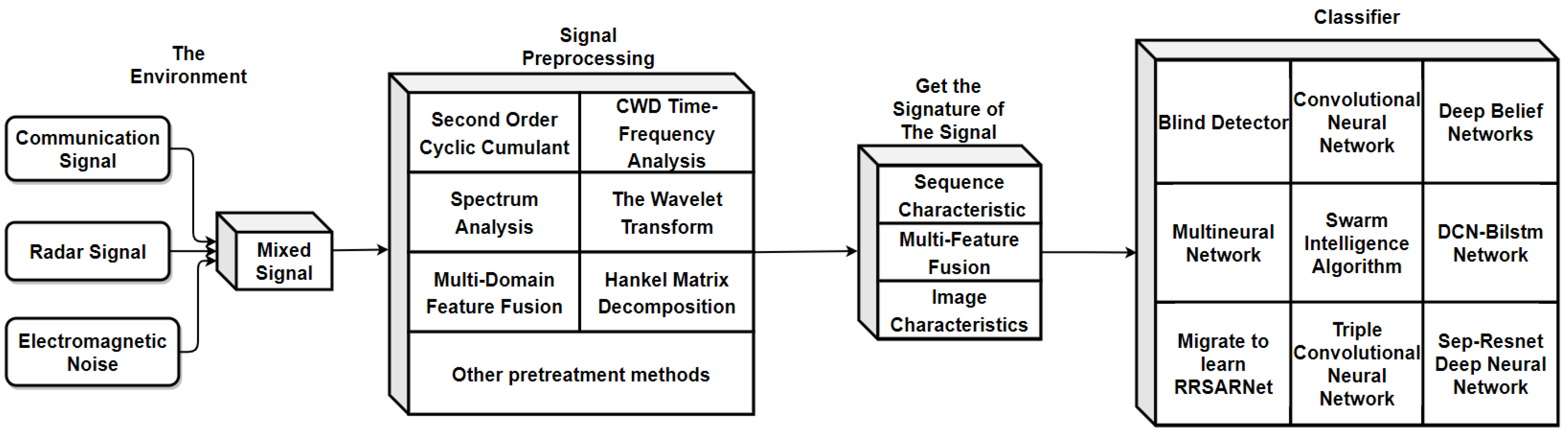
:1. Introduction
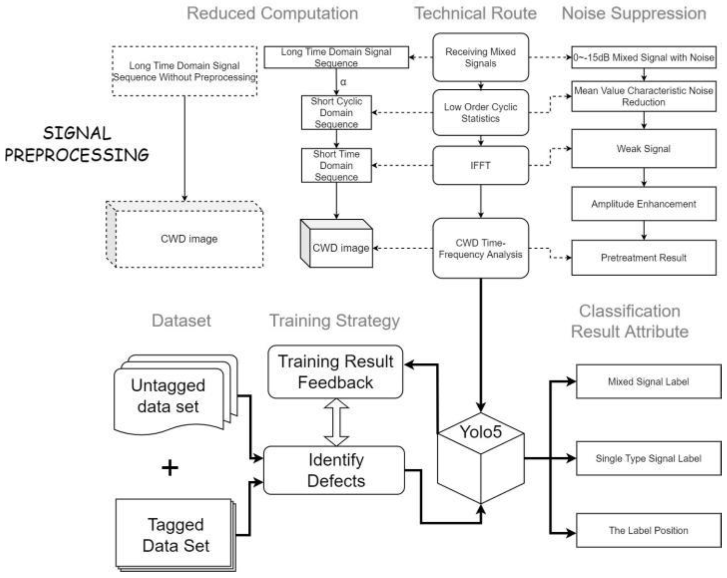
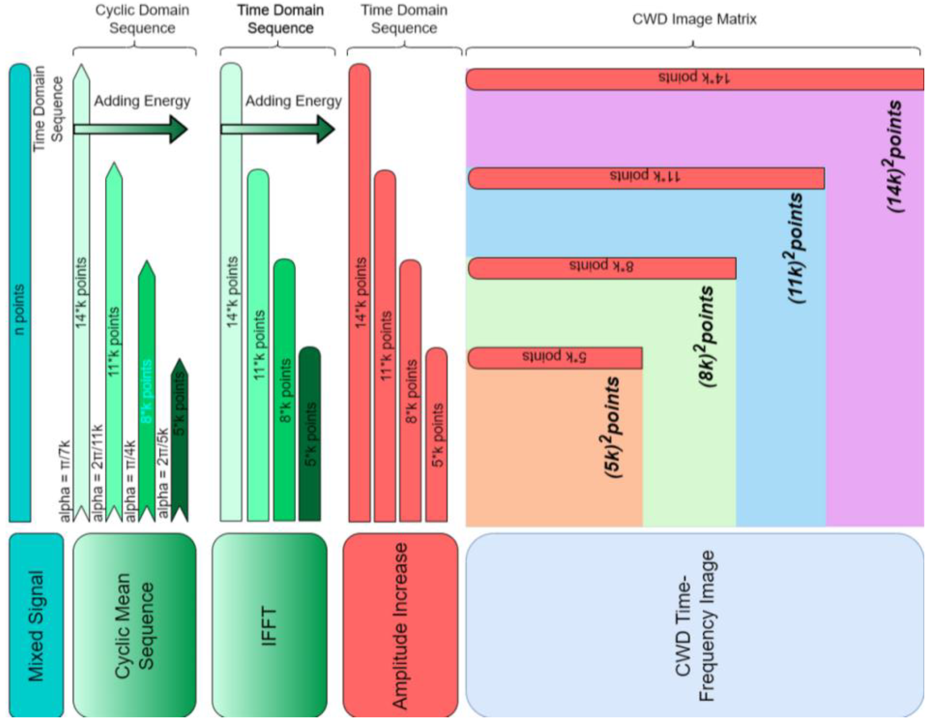
- Low-order cyclic statistics and CWD time-frequency analysis are used as the preprocessing methods for received signals. Using the granularity of the cycle frequency to adjust the resolution of the cycle mean, combined with the IFFT algorithm, can suppress the noise, reduce the amount of computation, and improve the real-time performance of the preprocessing algorithm.
- To mark and identify the modulation features of multiple signals on the time-frequency graph, we adopted the YOLOv5 deep neural network framework as the classifier. After training, the single recognition time is short, and multiple sub-signal features can be recognized simultaneously. The output result of the classifier is the basic premise of parameter estimation.
- To reduce the missed detection rate and identify the combination pattern of mixed signals, the labeled and unlabeled datasets are fused to train the classifier. Using different kinds and quantities of signals in the test can show the recognition defects of the classifier at different levels and support the subsequent optimization work.
2. Materials and Methods
2.1. Multisource Signal Preprocessing Method Based on Cyclic Mean and CWD Time-Frequency Analysis
2.1.1. Cyclic Mean Analysis of AM Signals
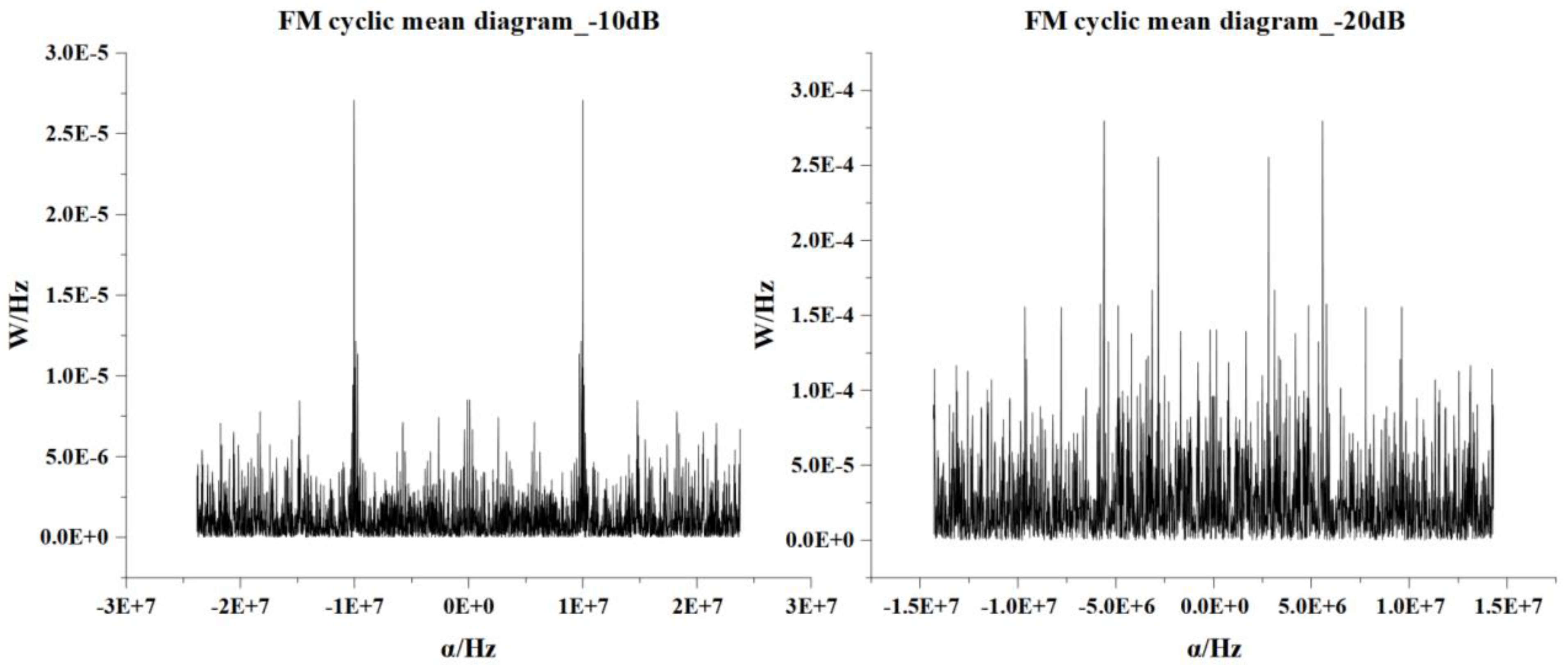
2.1.2. Cyclic Mean Analysis of the FM Signal
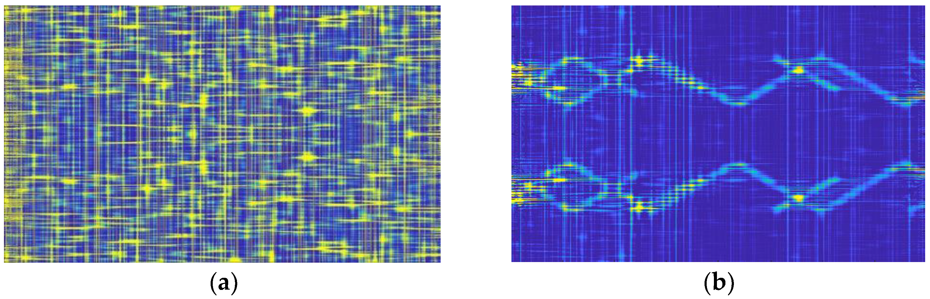
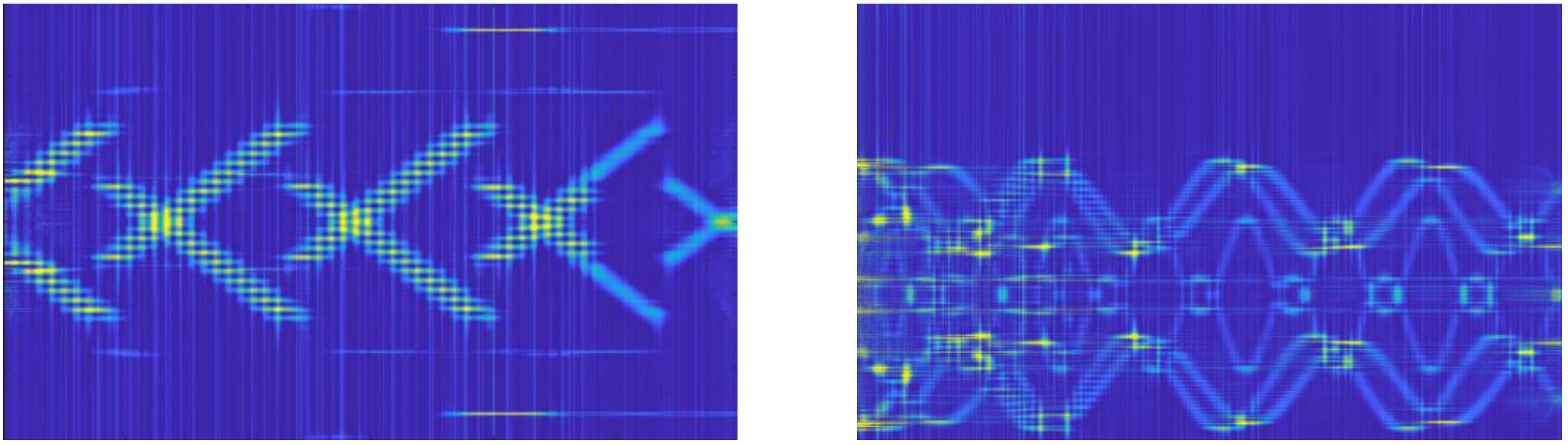
2.2. CWD Time-Frequency Analysis Image Generation
2.3. Comparison of the Results of the Preprocessing Algorithm
2.4. Computational Complexity of Preprocessing Algorithm
3. Multi-Emitter Signal Classification Model Based on a YOLO Deep Network
- An image is segmented into an S×S image matrix grid.
- If the center point of the predicted target falls within a grid, then the grid is bound to the current target.
- Within each grid, K borders containing the center point of the target are predicted.
- The target confidence of the border within each grid and the probability of each border area on multiple categories are calculated.
- The target window with low confidence is removed according to the threshold set.
- Non-maximum rejection (NMS) is used to remove redundant windows.
4. Research on Multi-Emitter Signal Sorting and Recognition Based on the Preprocessing Method and the YOLOv5 Model
4.1. Experimental Environment and Dataset Setup
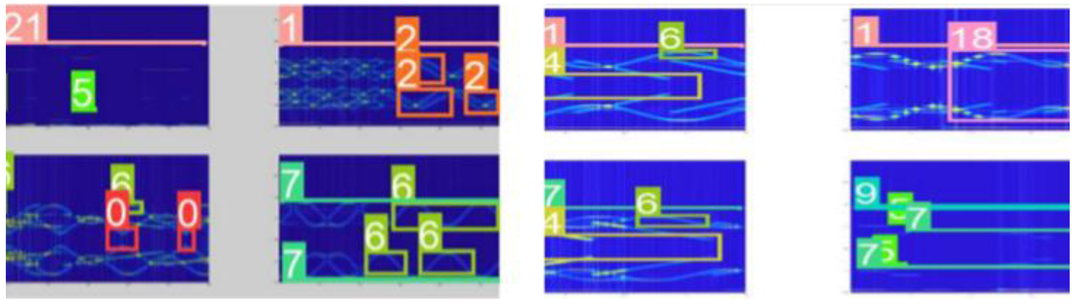
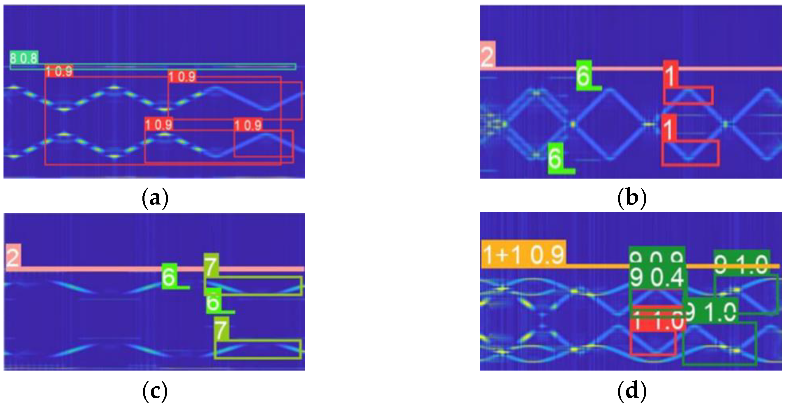
4.2. Experimental Analysis Based on the YOLOv5 Classification Model
5. Conclusions
6. Future Work Outlook
Author Contributions
Funding
Conflicts of Interest
Abbreviations
| AM | Amplitude modulation |
| BN | Batch Normalization |
| CBL | Convolution BatchNormalization Leakyrelu |
| CMWT | Complex Morlet Wavelet Transform |
| CNN | Convolutional Neural Network |
| CNN-DNN | Convolutional Neural Network-Deep Neural Networks |
| CSP | Cross Stage Paritial |
| CWD | Choi–Williams Distribution |
| DCN | Deformable Convolution Networks |
| BILSTM | Bi-Directional Long Short-Term Memory |
| FFT | Fast Fourier Transform |
| FM | Frequency Modulation |
| FM_SAW | Frequency Modulation Sawtooth wave |
| FM_TRI | Frequency Modulation Triangle wave |
| FPN | Feature Pyramid Networks |
| PAN | Path Aggregation Network |
| IFFT | Inverse Fast Fourier Transform |
| GIOU | Generalized Intersection over Union |
| LPI-NET | Lightweight Pyramid Inpainting Network |
| mAP | Mean Average Precision |
| NMS | Non Maximum Suppression |
| PWVD | Pseudo Wigner–Ville Distribution |
| RRSARNet | Radar Radio Sources Adaptive Recognition Network |
| SEP-ResNet | Channel-Separable Residual Neural Network |
| SFM | Sine Frequency Modulation |
| SiLU | Sigmoid Linear Unit |
| SNR | Signal-Noise Ratio |
| SPP | Spatial Pyramid Pooling |
| STFT | Short-time Fourier Transform |
| T-F | Time-Frequency |
| VHF | Very High Frequency |
| YOLO | You Only Look Once |
Appendix A. Pseudocode
| Pseudocode for Preprocessing Methods |
| Calculate the Cyclic Mean Input: Mixed Signal Sequences. Step 1: Settting the Value of alpha and attach,alpha = 2*pi/2000; It can be adjusted according to the desired noise-suppression effect and calculation time. Step 2: Setting length of the cyclic sequence,length = ceil(2*pi/alpha) + attach; Step 3: Construct the cyclic mean sequence space m for k = 0:length m(k + 1) = mean(signal.*exp(-1i*k*alpha*t)); |
| Calculate the IFFT of the Cyclic mean series Input: The Cyclic mean sequence of mixed-signal sequences. IFFT_signal = ifft(m_ga_add,n); This step should adjust the IFFT sequence length parameter n to reduce the CWD image’s computation time. |
| Run the CWD algorithm Input: Time domain signal sequence after IFFT operation. cwd_signal = tfrcw(IFFT_signal); CWD_FIG = image(cwd_signal); |
| Output: Mixed signal CWD image. |
| Pseudocode for YOLOv5 Detect Part (Important Steps) |
| Loading system libraries, setting the system environment. Input: The CWD picture of Mixed signals. Step 1:The size of the zoom image is [640 640] Step 2: Conf_value = 0.3 ## Boxes whose confidence is higher than 30% will be reserved. Step 3: Iou_value = 0.4 ## IOU boxes whose value is higher than this value can be reserved. Step 4: max_det = 10; ## Maximum number of targets. This value can change depending on the testing environment. |
| Predicting part Step 1:Use blank picture (0 matrix) prediction to accelerate the prediction process.Import single-label and multi-label datasets. Step 2: im/= 255 # 0–255 to 0.0–1.0 # Normalize the image. if len(im.shape) == 3: im = im[None] ## Add the 0th dimension. Step 3: pred = model(im, augment = augment, visualize = visualize) pred = non_max_suppression(pred,conf_thres,iou_thres,classes, agnostic_nms, max_det = max_det) ##Prediction box save and NMS Step 4: if len(det): # Rescale boxes from img_size to im0 size. det [:, :4] = scale_coords(im.shape [2:], det [:, :4], im0.shape).round() # Resize the annotated bounding_box to the same size as the original image (because the original image has been scaled up and down during training) # Print results Output the predicted time for each image. The accuracy distribution is returned according to the result of each prediction, and the lowest prediction accuracy category is output. |
| Output: Mixed signal CWD image with predict box. The target category. Degree of confidence. The box position. |
Appendix B. The Key Formula of Preprocessing Algorithm
References
- Yu, N.; Liang, W.; Shi, L.; Liu, W. A new blind detection algorithm based on cyclic statistics. Tactical Missile Technol. 2017, 6, 94–99. [Google Scholar] [CrossRef]
- Yang, F.; Li, Z.; Luo, Z. Research on VHF Band Signal Modulation Classification and Recognition Methods Based on Algorithm of First-Order Cyclic Moment. Telecom Sci. 2014, 30, 76–81. [Google Scholar]
- Lin, X.; Zhang, L.; Wu, Z.; Jiang, J. Modulation recognition method based on convolutional neural network and cyclic spectrum images. J. Terahertz Sci. Electron. Inf. 2021, 19, 617–622. [Google Scholar]
- Huynh-The, T.; Doan, V.-S.; Hua, C.-H.; Pham, Q.-V.; Nguyen, T.-V.; Kim, D.-S. Accurate LPI Radar Waveform Recognition with CWD-TFA for Deep Convolutional Network. IEEE Wirel. Commun. Lett. 2021, 10, 1638–1642. [Google Scholar] [CrossRef]
- Zhang, Q.; Ji, H.; Jin, Y. Cyclostationary Signals Analysis Methods Based on High-Dimensional Space Transformation Under Impulsive Noise. IEEE Signal Process. Lett. 2021, 28, 1724–1728. [Google Scholar] [CrossRef]
- Dong, P.; Wang, H.; Xiao, B.; Chen, Y.; Sheng, T.; Zhang, H.; Zhou, Y. Study for classification and recognition of radar emitter intra-pulse signals based on the energy cumulant of CWD. J. Ambient Intell. Humaniz. Comput. 2021, 12, 9809–9823. [Google Scholar] [CrossRef]
- Gao, J.; Wang, X.; Wu, R.; Xu, X. A New Modulation Recognition Method Based on Flying Fish Swarm Algorithm. IEEE Access 2021, 9, 76689–76706. [Google Scholar] [CrossRef]
- Zhang, L.; Liu, H.; Yang, X.; Jiang, Y.; Wu, Z. Intelligent Denoising-Aided Deep Learning Modulation Recognition With Cyclic Spectrum Features for Higher Accuracy. IEEE Trans. Aerosp. Electron. Syst. 2021, 57, 3749–3757. [Google Scholar] [CrossRef]
- Liu, K.; Gao, W.; Huang, Q. Automatic Modulation Recognition Based on a DCN-BiLSTM Network. Sensors 2021, 21, 1577. [Google Scholar] [CrossRef] [PubMed]
- Lang, P.; Fu, X.J.; Martorella, M.; Dong, J.; Qin, R.; Feng, C.; Zhao, C.X. RRSARNet: A Novel Network for Radar Radio Sources Adaptive Recognition. IEEE Trans. Veh. Technol. 2021, 70, 11483–11498. [Google Scholar] [CrossRef]
- Liu, L.; Li, X. Radar signal recognition based on triplet convolutional neural network. EURASIP J. Adv. Signal Process. 2021, 2021, 112. [Google Scholar] [CrossRef]
- Mao, Y.; Ren, W.; Yang, Z. Radar Signal Modulation Recognition Based on Sep-ResNet. Sensors 2021, 21, 7474. [Google Scholar] [CrossRef] [PubMed]
- Wang, C.; Wang, J.; Zhang, X. Automatic radar waveform recognition based on time-frequency analysis and convolutional neural network. In Proceedings of the 2017 IEEE International Conference on Acoustics, Speech and Signal Processing (ICASSP), New Orleans, LA, USA, 5–9 March 2017; pp. 2437–2441. [Google Scholar] [CrossRef]
- Zhang, M.; Diao, M.; Guo, L. Convolutional Neural Networks for Automatic Cognitive Radio Waveform Recognition. IEEE Access 2017, 5, 11074–11082. [Google Scholar] [CrossRef]
- Kong, S.-H.; Kim, M.; Hoang, L.M.; Kim, E. Automatic LPI Radar Waveform Recognition Using CNN. IEEE Access 2018, 6, 4207–4219. [Google Scholar] [CrossRef]
- Zhu, X.; Lyu, S.; Wang, X.; Zhao, Q. TPH-YOLOv5: Improved YOLOv5 Based on Transformer Prediction Head for Object Detection on Drone-captured Scenarios. In Proceedings of the IEEE/CVF International Conference on Computer Vision (ICCV) Workshops, Montreal, BC, Canada, 11–17 October 2021; pp. 2778–2788. [Google Scholar] [CrossRef]
- Zhao, Y.; Shi, Y.; Wang, Z. The Improved YOLOV5 Algorithm and Its Application in Small Target Detection. In Proceedings of the International Conference on Intelligent Robotics and Applications, Harbin, China, 1–3 August 2022; pp. 679–688. [Google Scholar] [CrossRef]
- Ye, J.; Yuan, Z.; Qian, C.; Li, X. CAA-YOLO: Combined-Attention-Augmented YOLO for Infrared Ocean Ships Detection. Sensors 2022, 22, 3782. [Google Scholar] [CrossRef]
- Ganesh, P.; Chen, Y.; Yang, Y.; Chen, D.M.; Winslett, M.; Soc, I.C. In YOLO-ReT: Towards High Accuracy Real-time Object Detection on Edge GPUs. In Proceedings of the 22nd IEEE/CVF Winter Conference on Applications of Computer Vision (WACV), Waikoloa, HI, USA, 4–8 January 2022; pp. 1311–1321. [Google Scholar]
- Guo, Q.; Liu, J.; Kaliuzhnyi, M. YOLOX-SAR: High-Precision Object Detection System Based on Visible and Infrared Sensors for SAR Remote Sensing. IEEE Sens. J. 2022, 22, 17243–17253. [Google Scholar] [CrossRef]
- Kosuge, A.; Suehiro, S.; Hamada, M.; Kuroda, T. mmWave-YOLO: A mmWave Imaging Radar-Based Real-Time Multiclass Object Recognition System for ADAS Applications. IEEE Trans. Instrum. Meas. 2022, 71, 2509810. [Google Scholar] [CrossRef]
- Song, Y.Y.; Xie, Z.Y.; Wang, X.W.; Zou, Y.Q. MS-YOLO: Object Detection Based on YOLOv5 Optimized Fusion Millimeter-Wave Radar and Machine Vision. IEEE Sens. J. 2022, 22, 15435–15447. [Google Scholar] [CrossRef]
- Hanna, S.; Dick, C.; Cabric, D. Signal Processing-Based Deep Learning for Blind Symbol Decoding and Modulation Classi-fication. IEEE J. Sel. Areas Commun. 2022, 40, 82–96. [Google Scholar] [CrossRef]
- Kim, J.; Harne, R.L.; Wang, K.-W. Online Signal Denoising Using Adaptive Stochastic Resonance in Parallel Array and its Application to Acoustic Emission Signals. J. Vib. Acoust. 2021, 144, 031006. [Google Scholar] [CrossRef]
- Xu, X.W.; Zhang, X.L.; Zhang, T.W.; Shi, J.; Wei, S.J.; Li, J.W. On-Board Ship Detection in SAR Images Based on L-YOLO. In Proceedings of the IEEE Radar Conference (RadarConf22), New York, NY, USA, 21–25 March 2022. [Google Scholar]
- Zhang, C.; Van der Baan, M. Signal Processing Using Dictionaries, Atoms, and Deep Learning: A Common Analysis-Synthesis Framework. Proc. IEEE 2022, 110, 454–475. [Google Scholar] [CrossRef]
- Xu, C.; Zhang, Y.; Fan, X.J.; Lan, X.J.; Ye, X.; Wu, T.N. An efficient fluorescence in situ hybridization (FISH)-based circulating ge-netically abnormal cells (CACs) identification method based on Multi-scale MobileNet-YOLO-V4. Quant. Imaging Med. Surg. 2022, 12, 2961–2976. [Google Scholar] [CrossRef] [PubMed]
- Shimura, T.; Umehira, M.; Watanabe, Y.; Wang, X.Y.; Takeda, S. An Advanced Wideband Interference Suppression Tech-nique using Envelope Detection and Sorting for Automotive FMCW Radar. In Proceedings of the IEEE Radar Conference (RadarConf22), New York, NY, USA, 21–25 March 2022. [Google Scholar]
- Ma, H.; Sun, Y.; Wu, N.; Li, Y. Relative Attributes-Based Generative Adversarial Network for Desert Seismic Noise Suppression. IEEE Geosci. Remote Sens. Lett. 2021, 19, 8023005. [Google Scholar] [CrossRef]
- Klintberg, J.; McKelvey, T.; Dammert, P. A Parametric Approach to Space-Time Adaptive Processing in Bistatic Radar Systems. IEEE Trans. Aerosp. Electron. Syst. 2021, 58, 1149–1160. [Google Scholar] [CrossRef]


| Category | Configuration |
|---|---|
| CPU | Intel(R) Core(TM)i7-10700K @3.80 GHz |
| GPU | NVIDIA Tesla V100 32 GB |
| Operating System | Linux |
| Deep Learning Framework | Pytorch 1.8.1 |
| Programming Language | Python 3.8 |
| Dependent Package | CUDA 11.1.1 |
| Carrier Fre | Mod Fre | Sample Fre | SNR | Special PAR | |
|---|---|---|---|---|---|
| FM_TRI | 1 GHz | 100 kHz | 4 GHz | −15~0 Step | None |
| FM_SAW | 1 GHz | 100 kHz | 4 GHz | −15~0 Step | None |
| SFM | 1 GHz | 100 kHz | 4 GHz | −15~0 Step | None |
| PULSE | 2 GH z | 100 kHz | 4 GHz | −15~0 Step | Duty Ratio 50% |
| AM | 800 M–1.5 GHz | 100 kHz | 4 GHz | −15~0 Step | 50% Mod Rate |
| Fre_Agility | 800 M–1.5 MHz | 100 kHz | 4 GHz | −15~0 Step | 5 Frequencies |
| Biphase Coding | 1 GHz | 100 kHz | 4 GHz | −15~0 Step | Duty Ratio 50% |
| Size | Precision (%) | GFLOPs | Parameters | Data Pictures | Training Time (min) |
|---|---|---|---|---|---|
| YOLOv5n | 42.3% | 6.0 | 2.9 M | 3500 | 376 |
| YOLOv5s | 53% | 17.1 | 7.7 M | 3500 | 1170 |
| YOLOv5m | 89.2% | 43.6 | 21.4 M | 3500 | 1982 |
| YOLOv5x | 96.5% | 219.7 | 219.0 M | 3500 | 3000 |
| YOLOv5n | YOLOv5s | YOLOv5x | R-CNN | SPPNet | Fast-R-CNN |
|---|---|---|---|---|---|
| 0.37 s | 0.4 s | 0.45 s | 47 s | 2.3 s | 0.32 s |
Publisher’s Note: MDPI stays neutral with regard to jurisdictional claims in published maps and institutional affiliations. |
© 2022 by the authors. Licensee MDPI, Basel, Switzerland. This article is an open access article distributed under the terms and conditions of the Creative Commons Attribution (CC BY) license (https://creativecommons.org/licenses/by/4.0/).
Share and Cite
Huang, D.; Yan, X.; Hao, X.; Dai, J.; Wang, X. Low SNR Multi-Emitter Signal Sorting and Recognition Method Based on Low-Order Cyclic Statistics CWD Time-Frequency Images and the YOLOv5 Deep Learning Model. Sensors 2022, 22, 7783. https://doi.org/10.3390/s22207783
Huang D, Yan X, Hao X, Dai J, Wang X. Low SNR Multi-Emitter Signal Sorting and Recognition Method Based on Low-Order Cyclic Statistics CWD Time-Frequency Images and the YOLOv5 Deep Learning Model. Sensors. 2022; 22(20):7783. https://doi.org/10.3390/s22207783
Chicago/Turabian StyleHuang, Dingkun, Xiaopeng Yan, Xinhong Hao, Jian Dai, and Xinwei Wang. 2022. "Low SNR Multi-Emitter Signal Sorting and Recognition Method Based on Low-Order Cyclic Statistics CWD Time-Frequency Images and the YOLOv5 Deep Learning Model" Sensors 22, no. 20: 7783. https://doi.org/10.3390/s22207783
APA StyleHuang, D., Yan, X., Hao, X., Dai, J., & Wang, X. (2022). Low SNR Multi-Emitter Signal Sorting and Recognition Method Based on Low-Order Cyclic Statistics CWD Time-Frequency Images and the YOLOv5 Deep Learning Model. Sensors, 22(20), 7783. https://doi.org/10.3390/s22207783