Wi-Fi Fingerprint-Based Indoor Localization Method via Standard Particle Swarm Optimization


Abstract
:1. Introduction
- A two-panel fingerprint homogeneity model was adopted to characterize fingerprint similarity. In addition to considering both the real distance and direction difference of two fingerprints, this study proposes another combination, Euclidean metric and cosine distance, which was used in the system for a more robust performance.
- An effective application of a standard particle swarm optimization (SPSO) algorithm for Wi-Fi fingerprint-based indoor localization is proposed to improve the localization accuracy.
- Experiments on data sets and tests were conducted in a real-world environment and the results were compared with those obtained using other classical localization methods, thereby verifying the effectiveness of the proposed localization method.
2. Related Work
2.1. Wi-Fi-Based Indoor Localization
- Triangulation method. This method relies on the measurement of distance. Thereafter, the location estimation is obtained through geometric calculation. Classical triangulation localization methods [24] include time of arrival (TOA), time difference of arrival (TDOA), and angle of arrival (AOA). TOA is a measurement method to calculate the distance between the terminal device and the Wi-Fi access point (AP) by recording the unidirectional or bidirectional arrival time of Wi-Fi signals between the their terminals. However, it requires the precise synchronization of the time stamps at the transmitter and receiver. TDOA uses the characteristic that two focal distances on a hyperbola remain fixed. Based on the arrival time difference between the terminal device and different APs, using the hyperbolic equation, the location of the localization point can be solved. In contrast to TOA, TDOA reduces the time synchronization requirement, but accurate time measurement is a limiting factor. Moreover, it is susceptible to non-line-of-sight (NLOS) problems. AOA involves obtaining positions through azimuth angle measurements. It eliminates the need for accurate time synchronization between devices and requires a small number of base stations. However, it measures the signal transmission angle, which requires localization equipment carrying an antenna array device, thereby increasing the difficulty of its popularization.
- Wi-Fi fingerprint-based method. This method utilizes the mapping correlation between Wi-Fi signal characteristics and physical locations. In the ideal localization environment, each physical location should have a unique and distinguishable fingerprint [23]. Generally, in this method, an indoor-location area is divided into a series of discrete grid spaces in advance to obtain the radio fingerprint map. Further, in the Offline phase, the Wi-Fi received signal strength (RSS) from different access points (APs) are collected on each reference point (RPs) of discrete grid points. Consequently, combining the physical coordinates of RPs, the fingerprint database is constructed. Thus, a received Wi-Fi fingerprint can determine the most similar fingerprint of database in the Online phase, and, subsequently, the corresponding coordinate can be estimated.
- Deterministic methods. These algorithms directly use the one-to-one mapping relationship between Wi-Fi fingerprint and physical location and estimate the unknown position based on the closest fingerprint location in signal space. K-nearest neighbor (KNN) [25] is one such example. The method is to determine the K most similar Wi-Fi fingerprints from a database using the Euclidean distance, and then calculate the average of the K corresponding physical locations. Ma et al. [26] improved the KNN algorithm and proposed the WKNN algorithm, which used a weighted average for location estimation. Neural network (NN) algorithms [27], such as the multi-layer neural network [28], have also been applied to Wi-Fi fingerprint-based localization but with high computational cost. NN obtains the mapping relationship between a fingerprint and physical position after considerable training, then uses it to predict the unknown position. Certain other, more deterministic, algorithms such as support vector machine [29], random forests [30] and linear discriminant analysis [31] are also used in localization.
- Probabilistic methods. Contrary to deterministic algorithms, probabilistic methods employ the probability density function, which characterizes changes in RSS. The key is to predict the possibility of relationships between real-time data and the coordinates of RPs. Horus [32] estimated the unknown position using a probabilistic model considering the signal distribution in the site. Bayesian network [33], expectation maximization [34], Gaussian process [35] and conditional random field [36] are also effective probabilistic algorithms.
2.2. Particle Swarm Optimization
3. System Overview
3.1. Preliminary
3.2. Two-Panel Fingerprint-Homogeneity Model
3.3. SPSO Algorithm for Localization
| Algorithm 1 The algorithm procedure of localization. |
| Input: |
| The offline fingerprints data and the coordinates data ; |
| The query fingerprint ; |
| Output: |
| The location estimation of the query fingerprint. |
|
4. Experiments and Analysis
4.1. Experimental Setup
4.2. Performance Metric
4.3. Results and Discussion
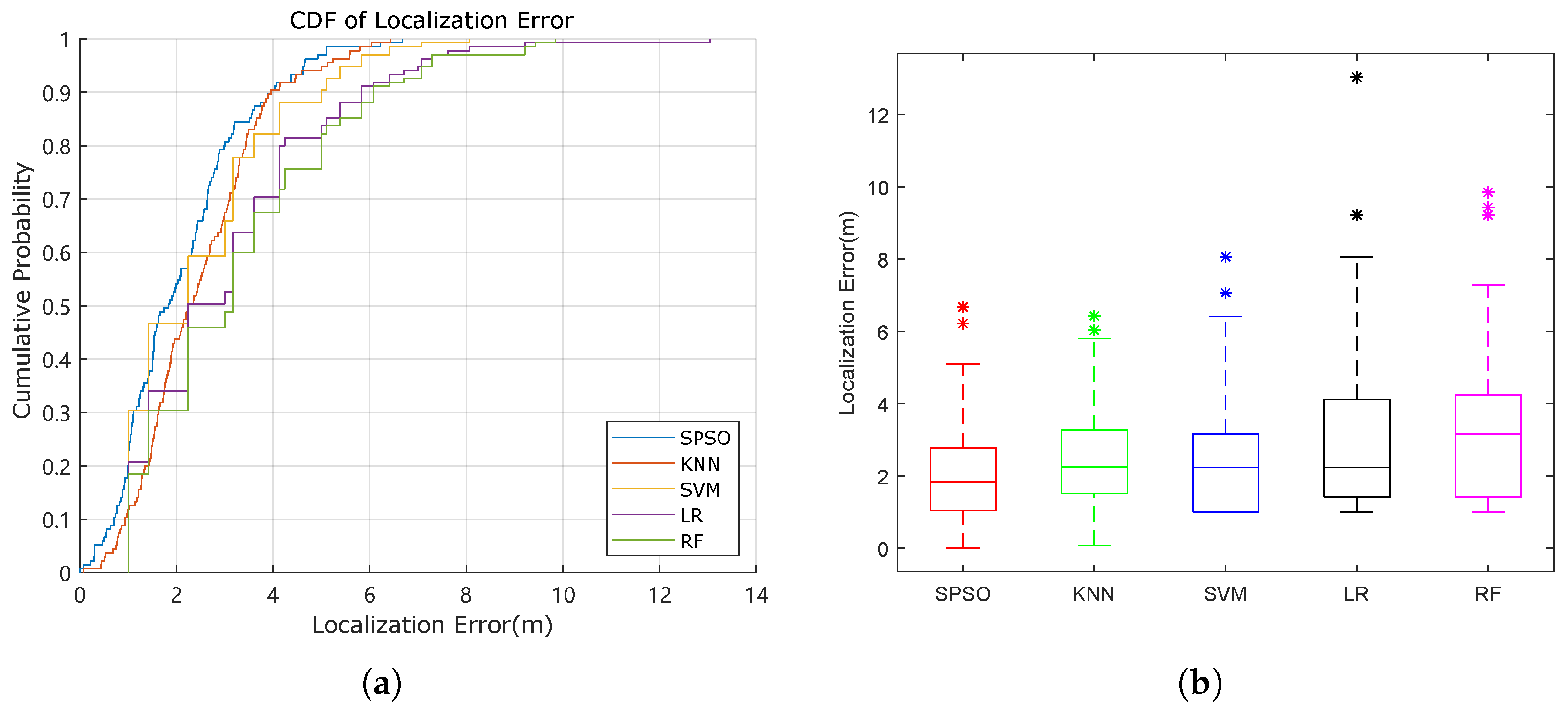
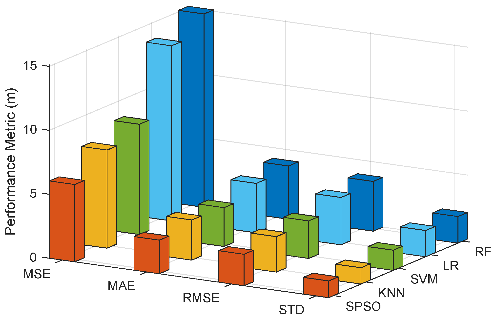
4.3.1. Performance Comparison of Different Methods
4.3.2. Model Analysis
5. Conclusions
Author Contributions
Funding
Institutional Review Board Statement
Informed Consent Statement
Data Availability Statement
Conflicts of Interest
Abbreviations
| ANN | Artificial neural network |
| AOA | Angle of arrival |
| AP | Access point |
| GPS | Global positioning system |
| IMU | Inertial measurement units |
| IoT | Internet-of-Things |
| KNN | K-nearest neighbor |
| LR | Linear regression |
| MAE | Mean absolute error |
| MSE | Mean square error |
| NLOS | Non-line of sight |
| NN | Neural network |
| PSO | Particle swarm optimization |
| RF | Random forests |
| RFID | Radio frequency identification |
| RMSE | Root mean square error |
| RP | Reference point |
| RSS | Received signal strength |
| SPSO | Standard particle swarm optimization |
| STD | Standard deviation |
| SVM | Support vector machine |
| TDOA | Time difference of arrival |
| TOA | Time of arrival |
| UWB | Ultra wide band |
| WKNN | Weighted k-nearest neighbor |
References
- Khan, M.A.; Saboor, A.; Kim, H.C.; Park, H. A Systematic Review of Location Aware Schemes in the Internet of Things. Sensors 2021, 21, 3228. [Google Scholar] [CrossRef] [PubMed]
- Jagannath, J.; Polosky, N.; Jagannath, A.; Restuccia, F.; Melodia, T. Machine learning for wireless communications in the Internet of Things: A comprehensive survey. Ad Hoc Netw. 2019, 93, 101913. [Google Scholar] [CrossRef] [Green Version]
- Singh, N.; Choe, S.; Punmiya, R. Machine Learning Based Indoor Localization Using Wi-Fi RSSI Fingerprints: An Overview. IEEE Access 2021, 9, 127150–127174. [Google Scholar] [CrossRef]
- Geok, T.K.; Aung, K.Z.; Aung, M.S.; Soe, M.T.; Abdaziz, A.; Liew, C.P.; Hossain, F.; Tso, C.P.; Yong, W.H. Review of Indoor Positioning: Radio Wave Technology. Appl. Sci. 2021, 11, 279. [Google Scholar] [CrossRef]
- Liu, F.; Liu, J.; Yin, Y.Q.; Wang, W.H.; Hu, D.H.; Chen, P.P.; Niu, Q. Survey on WiFi-based indoor positioning techniques. IET Commun. 2020, 14, 1372–1383. [Google Scholar] [CrossRef]
- Tomazic, S.; Skrjanc, I. An Automated Indoor Localization System for Online Bluetooth Signal Strength Modeling Using Visual-Inertial SLAM. Sensors 2021, 21, 2857. [Google Scholar] [CrossRef]
- Poulose, A.; Han, D.S. UWB Indoor Localization Using Deep Learning LSTM Networks. Appl. Sci. 2020, 10, 6290. [Google Scholar] [CrossRef]
- Guan, W.P.; Chen, S.H.; Wen, S.S.; Tan, Z.Q.; Song, H.Z.; Hou, W.Y. High-Accuracy Robot Indoor Localization Scheme Based on Robot Operating System Using Visible Light Positioning. IEEE Photonics J. 2020, 12, 7901716. [Google Scholar] [CrossRef]
- Bianchi, V.; Ciampolini, P.; De Munari, I. RSSI-Based Indoor Localization and Identification for ZigBee Wireless Sensor Networks in Smart Homes. IEEE Trans. Instrum. Meas. 2019, 68, 566–575. [Google Scholar] [CrossRef]
- Morar, A.; Moldoveanu, A.; Mocanu, I.; Moldoveanu, F.; Radoi, I.E.; Asavei, V.; Gradinaru, A.; Butean, A. A Comprehensive Survey of Indoor Localization Methods Based on Computer Vision. Sensors 2020, 20, 2641. [Google Scholar] [CrossRef]
- Motroni, A.; Buffi, A.; Nepa, P. A Survey on Indoor Vehicle Localization through RFID Technology. IEEE Access 2021, 9, 17921–17942. [Google Scholar] [CrossRef]
- Poulose, A.; Eyobu, O.S.; Han, D.S. An Indoor Position-Estimation Algorithm Using Smartphone IMU Sensor Data. IEEE Access 2019, 7, 11165–11177. [Google Scholar] [CrossRef]
- Ashraf, I.; Kang, M.Y.; Hur, S.; Park, Y. MINLOC: Magnetic Field Patterns-Based Indoor Localization Using Convolutional Neural Networks. IEEE Access 2020, 8, 66213–66227. [Google Scholar] [CrossRef]
- Simka, M.; Polak, L. On the RSSI-Based Indoor Localization Employing LoRa in the 2.4 GHz ISM Band. Radioengineering 2022, 31, 135–143. [Google Scholar] [CrossRef]
- Zafari, F.; Gkelias, A.; Leung, K.K. A Survey of Indoor Localization Systems and Technologies. IEEE Commun. Surv. Tutor. 2019, 21, 2568–2599. [Google Scholar] [CrossRef] [Green Version]
- Holm, S. Hybrid Ultrasound-RFID Indoor Positioning: Combining the Best of Both Worlds. In Proceedings of the IEEE International Conference on RFID, Orlando, FL, USA, 27–28 April 2009; pp. 155–162. [Google Scholar]
- Feng, D.Q.; Wang, C.Q.; He, C.L.; Zhuang, Y.; Xia, X.G. Kalman-Filter-Based Integration of IMU and UWB for High-Accuracy Indoor Positioning and Navigation. IEEE Internet Things J. 2020, 7, 3133–3146. [Google Scholar] [CrossRef]
- Obeidat, H.; Shuaieb, W.; Obeidat, O.; Abd-Alhameed, R. A Review of Indoor Localization Techniques and Wireless Technologies. Wirel. Pers. Commun. 2021, 119, 289–327. [Google Scholar] [CrossRef]
- Zhang, X.; Sun, W.; Zheng, J.; Xue, M.; Tang, C.; Zimmermann, R. Towards Floor Identification and Pinpointing Position: A Multistory Localization Model with WiFi Fingerprint. Int. J. Control Autom. Syst. 2022, 20, 1484–1499. [Google Scholar] [CrossRef]
- Bratton, D.; Kennedy, J. Defining a standard for particle swarm optimization. In Proceedings of the IEEE Swarm Intelligence Symposium, Honolulu, HI, USA, 1–5 April 2007; pp. 120–127. [Google Scholar]
- Lomayev, A.; Da Silva, C.R.C.M.; Maltsev, A.; Cordeiro, C.; Sadrl, A.S. Passive Presence Detection Algorithm for Wi-Fi Sensing. Radioengineering 2020, 29, 540–547. [Google Scholar] [CrossRef]
- Li, J.; Sharma, A.; Mishra, D.; Seneviratne, A. Fire Detection Using Commodity WiFi Devices. In Proceedings of the IEEE Global Communications Conference (GLOBECOM), Madrid, Spain, 7–11 December 2021; pp. 1–6. [Google Scholar]
- He, S.N.; Chan, S.H.G. Wi-Fi Fingerprint-Based Indoor Positioning: Recent Advances and Comparisons. IEEE Commun. Surv. Tutor. 2016, 18, 466–490. [Google Scholar] [CrossRef]
- Yang, C.C.; Shao, H.R. WiFi-Based Indoor Positioning. IEEE Commun. Mag. 2015, 53, 150–157. [Google Scholar] [CrossRef]
- Bahl, P.; Padmanabhan, V.N. RADAR: An In-Building RF-based User Location and Tracking System. In Proceedings of the Nineteenth Annual Joint Conference of the IEEE Computer and Communications Societies (Cat. No.00CH37064), Tel Aviv, Israel, 26–30 March 2000; Volume 2, pp. 775–784. [Google Scholar]
- Ma, R.; Guo, Q.; Hu, C.; Xue, J. An Improved WiFi Indoor Positioning Algorithm by Weighted Fusion. Sensors 2015, 15, 21824–21843. [Google Scholar] [CrossRef] [PubMed]
- Wang, B.F.; Zhu, H.; Xu, M.M.; Wang, Z.M.; Song, X.D. Analysis and improvement for Fingerprinting-based Localization Algorithm based on Neural Network. In Proceedings of the 15th International Conference on Computational Intelligence and Security (CIS), Macao, China, 13–16 December 2019; pp. 82–86. [Google Scholar]
- Dai, H.; Ying, W.H.; Xu, J. Multi-layer neural network for received signal strength-based indoor localisation. IET Commun. 2016, 10, 717–723. [Google Scholar] [CrossRef]
- Chriki, A.; Touati, H.; Snoussi, H. SVM-Based Indoor Localization in Wireless Sensor Networks. In Proceedings of the 13th International Wireless Communications and Mobile Computing Conference (IWCMC), Valencia, Spain, 26–30 June 2017; pp. 1144–1149. [Google Scholar]
- Guo, X.S.; Ansari, N.; Li, L.; Li, H.Y. Indoor Localization by Fusing a Group of Fingerprints Based on Random Forests. IEEE Internet Things J. 2018, 5, 4686–4698. [Google Scholar] [CrossRef] [Green Version]
- Luo, J.; Zhang, Z.Y.; Wang, C.; Liu, C.; Xiao, D.G. Indoor Multifloor Localization Method Based on WiFi Fingerprints and LDA. IEEE Trans. Ind. Inform. 2019, 15, 5225–5234. [Google Scholar] [CrossRef]
- Youssef, M.A.; Agrawala, A.; Shankar, A.U. WLAN location determination via clustering and probability distributions. In Proceedings of the 1st IEEE International Conference on Pervasive Computing and Communications, Fort Worth, TX, USA, 26 March 2003; pp. 143–150. [Google Scholar]
- Madigan, D.; Elnahrawy, E.; Martin, R.P.; Ju, W.F.; Krishnan, P.; Krishnakumar, A.S. Bayesian indoor positioning systems. In Proceedings of the 24th Annual Joint Conference of the IEEE Computer and Communications Societies, Miami, FL, USA, 13–17 March 2005; pp. 1217–1227. [Google Scholar]
- Guo, X.S.; Li, L.; Xu, F.; Ansari, N. Expectation Maximization Indoor Localization Utilizing Supporting Set for Internet of Things. IEEE Internet Things J. 2019, 6, 2573–2582. [Google Scholar] [CrossRef]
- Sun, W.; Xue, M.; Yu, H.S.; Tang, H.W.; Lin, A.P. Augmentation of Fingerprints for Indoor WiFi Localization Based on Gaussian Process Regression. IEEE Trans. Veh. Technol. 2018, 67, 10896–10905. [Google Scholar] [CrossRef]
- Lee, Y.H.; Lin, C.S. WiFi Fingerprinting for Indoor Room Localization Based on CRF Prediction. In Proceedings of the 3rd International Symposium on Computer, Consumer and Control (IS3C), Xi’an, China, 4–6 July 2016; pp. 315–318. [Google Scholar]
- Luo, M.; Zheng, J.; Sun, W.; Zhang, X. WiFi-based Indoor Localization Using Clustering and Fusion Fingerprint. In Proceedings of the 2021 40th Chinese Control Conference (CCC), Shanghai, China, 26–28 July 2021; pp. 3480–3485. [Google Scholar]
- James Kennedy, R.E. Particle swarm optimization. In Proceedings of the ICNN’95—International Conference on Neural Networks, Perth, WA, Australia, 27 November–1 December 1995; Volume 4, pp. 1942–1948. [Google Scholar]
- Abed, A.K.; Abdel-Qader, I. Access Point Selection Using Particle Swarm Optimization in Indoor Positioning Systems. In Proceedings of the NAECON 2018—IEEE National Aerospace and Electronics Conference, Dayton, OH, USA, 23–26 July 2018; pp. 403–410. [Google Scholar]
- Tewolde, G.S.; Kwon, J. Efficient WiFi-Based Indoor Localization Using Particle Swarm Optimization. In Proceedings of the Advances in Swarm Intelligence, Dalian, China, 26–28 July 2011; pp. 203–211. [Google Scholar]
- Wang, Y. User positioning with particle swarm optimization. In Proceedings of the 2017 International Conference on Indoor Positioning and Indoor Navigation (IPIN), Sapporo, Japan, 18–21 September 2017; pp. 1–5. [Google Scholar]
- Bi, J.; Cao, H.; Yao, G.; Chen, Z.; Cao, J.; Gu, X. Indoor Fingerprint Positioning Method with Standard Particle Swarm Optimization. In Proceedings of the China Satellite Navigation Conference (CSNC 2021), Jakarta, Indonesia, 24–25 October 2021; Springer: Singapore; pp. 403–412. [Google Scholar]
- Li, N.; Chen, J.; Yuan, Y.; Tian, X.; Han, Y.; Xia, M. A Wi-Fi Indoor Localization Strategy Using Particle Swarm Optimization Based Artificial Neural Networks. Int. J. Distrib. Sens. Netw. 2016, 12, 4583147. [Google Scholar] [CrossRef] [Green Version]
- Lu, X.M.; Qiu, Y.; Yuan, W.L.; Yang, F. An Improved Dynamic Prediction Fingerprint Localization Algorithm Based On KNN. In Proceedings of the 6th International Conference on Instrumentation and Measurement, Computer, Communication and Control (IMCCC), Harbin, China, 21–23 July 2016; pp. 289–292. [Google Scholar]
- Hernandez, N.; Ocana, M.; Alonso, J.M.; Kim, E. Continuous Space Estimation: Increasing WiFi-Based Indoor Localization Resolution without Increasing the Site-Survey Effort. Sensors 2017, 17, 147. [Google Scholar] [CrossRef]
- Hoang, M.K.; Schmalenstroeer, J.; Haeb-Umbach, R. Aligning Training Models With Smartphone Properties In Wifi Fingerprinting Based Indoor Localization. In Proceedings of the 40th IEEE International Conference on Acoustics, Speech, and Signal Processing (ICASSP), South Brisbane, QLD, Australia, 19–24 April 2015; pp. 1981–1985. [Google Scholar]
- Lee, S.; Moon, N. Location recognition system using random forest. J. Ambient. Intell. Humaniz. Comput. 2018, 9, 1191–1196. [Google Scholar] [CrossRef]


| Notations | Descriptions |
|---|---|
| Set of Access Points | |
| M | Number of Access Points |
| Set of Reference Points for Training and its ith Point | |
| Set of Reference Points for Test and its ith Point | |
| Training Fingerprints and the ith Training Fingerprint | |
| Test Fingerprints and the ith Test Fingerprint | |
| Received Signal Strength of ith RP from jth AP | |
| Number of Training Fingerprints | |
| Number of Test Fingerprints/Query Fingerprints | |
| The Query Fingerprint in the Online Phase | |
| Euclidean and Cosine Distance of Two Vectors | |
| The Simlarity Characterization of Two Vectors according to Euclidean and Cosine Distance | |
| K | Number of the Most Similar Training Fingerprints to Test Fingerprint |
| The kth Most Similar Training Fingerprint to Query Fingerprint | |
| The Location Coefficients of Location Estimation according to Euclidean and Cosine Distance | |
| D | Dimension of the Particles |
| Size of Particle Swarm/Number of Particles | |
| Acceleration Factors in SPSO | |
| Inertia weight for the tth Iteration in SPSO | |
| Velocity vector and its dth Dimension Velocity of the ith particle in the tth iteration | |
| Position vector and its dth Dimension Position of the ith particle in the tth iteration | |
| Historical Optimal Solution of Each Particle and its dth Dimension Value in the tth iteration | |
| Historical Global Optimal Solution of Particle Swarm and its dth Dimension Value in the tth iteration | |
| Maximum Iterations |
| Performance Metrics | SPSO | KNN | SVM | LR | RF |
|---|---|---|---|---|---|
| MSE (m) | 6.0433 | 7.6718 | 8.6224 | 13.6885 | 15.1111 |
| MAE (m) | 2.6288 | 3.1389 | 3.0370 | 3.8667 | 4.1630 |
| RMSE (m) | 2.4583 | 2.7698 | 2.9364 | 3.6998 | 3.8873 |
| STD (m) | 1.3076 | 1.2758 | 1.5789 | 2.0518 | 2.0777 |
| Accuracy (m) | 2.0817 | 2.4585 | 2.4757 | 3.0788 | 3.2855 |
| 25% Error (m) | 1.0122 | 1.5104 | 1.0000 | 1.4142 | 1.4142 |
| 50% Error (m) | 1.8329 | 2.2451 | 2.2361 | 2.2361 | 3.1623 |
| 75% Error (m) | 2.7831 | 3.2639 | 3.1623 | 4.1231 | 4.2426 |
| Improvement in RMSE | / | 11.25% | 16.28% | 33.56% | 36.76% |
| Improvement in Accuracy | / | 15.32% | 15.91% | 32.38% | 36.64% |
| Time Consumption (s) | <0.05 | <0.01 | <0.001 | <0.001 | <0.01 |
| No. | Distance Metrics | Weight | Accuracy (m) | RMSE (m) | STD (m) |
|---|---|---|---|---|---|
| 1 | Euclidean Metric | 1 | 2.3600 | 2.6768 | 1.2631 |
| 2 | 2.2261 | 2.6311 | 1.4026 | ||
| 3 | 2.3555 | 2.7770 | 1.4708 | ||
| 2 | Mahalanobis Distance | 1 | 4.0090 | 4.7974 | 2.6350 |
| 2 | 3.8229 | 4.5652 | 2.4952 | ||
| 3 | 3.6852 | 4.5175 | 2.6128 | ||
| 3 | Correlation Metric | 1 | 2.3250 | 2.6555 | 1.2831 |
| 2 | 2.4336 | 2.7733 | 1.3299 | ||
| 3 | 2.4509 | 2.8180 | 1.3909 | ||
| 4 | Cosine Distance | 1 | 2.2089 | 2.5444 | 1.2629 |
| 2 | 2.3378 | 2.6648 | 1.2789 | ||
| 3 | 2.3857 | 2.7082 | 1.2818 | ||
| 5 | Euc and Mahal | 1 | 2.6692 | 3.1911 | 1.7490 |
| 2 | 2.4599 | 2.9309 | 1.5934 | ||
| 3 | 2.4903 | 3.0561 | 1.7714 | ||
| 6 | Euc and Cor | 1 | 2.2177 | 2.5252 | 1.2077 |
| 2 | 2.1432 | 2.5172 | 1.3203 | ||
| 3 | 2.1707 | 2.5491 | 1.3364 | ||
| 7 | Euc and Cos | 1 | 2.2584 | 2.5892 | 1.2664 |
| 2 | 2.1516 | 2.5497 | 1.3681 | ||
| 3 | 2.1128 | 2.4766 | 1.2922 | ||
| 8 | Mahal and Cor | 1 | 2.5656 | 3.0026 | 1.5599 |
| 2 | 2.6912 | 3.1527 | 1.6422 | ||
| 3 | 2.6900 | 3.2157 | 1.7621 | ||
| 9 | Mahal and Cos | 1 | 2.5490 | 2.9419 | 1.4689 |
| 2 | 2.7242 | 3.1993 | 1.6775 | ||
| 3 | 2.6901 | 3.2255 | 1.7797 | ||
| 10 | Cor and Cos [19] | 1 | 2.2559 | 2.5988 | 1.2902 |
| 2 | 2.2831 | 2.6071 | 1.2587 | ||
| 3 | 2.3244 | 2.6445 | 1.2612 |
Publisher’s Note: MDPI stays neutral with regard to jurisdictional claims in published maps and institutional affiliations. |
© 2022 by the authors. Licensee MDPI, Basel, Switzerland. This article is an open access article distributed under the terms and conditions of the Creative Commons Attribution (CC BY) license (https://creativecommons.org/licenses/by/4.0/).
Share and Cite
Zheng, J.; Li, K.; Zhang, X. Wi-Fi Fingerprint-Based Indoor Localization Method via Standard Particle Swarm Optimization. Sensors 2022, 22, 5051. https://doi.org/10.3390/s22135051
Zheng J, Li K, Zhang X. Wi-Fi Fingerprint-Based Indoor Localization Method via Standard Particle Swarm Optimization. Sensors. 2022; 22(13):5051. https://doi.org/10.3390/s22135051
Chicago/Turabian StyleZheng, Jin, Kailong Li, and Xing Zhang. 2022. "Wi-Fi Fingerprint-Based Indoor Localization Method via Standard Particle Swarm Optimization" Sensors 22, no. 13: 5051. https://doi.org/10.3390/s22135051
APA StyleZheng, J., Li, K., & Zhang, X. (2022). Wi-Fi Fingerprint-Based Indoor Localization Method via Standard Particle Swarm Optimization. Sensors, 22(13), 5051. https://doi.org/10.3390/s22135051