
A Review of Computer Vision-Based Structural Deformation Monitoring in Field Environments


Abstract
1. Introduction
2. System Composition
2.1. Camera
2.2. Lens
2.3. Target
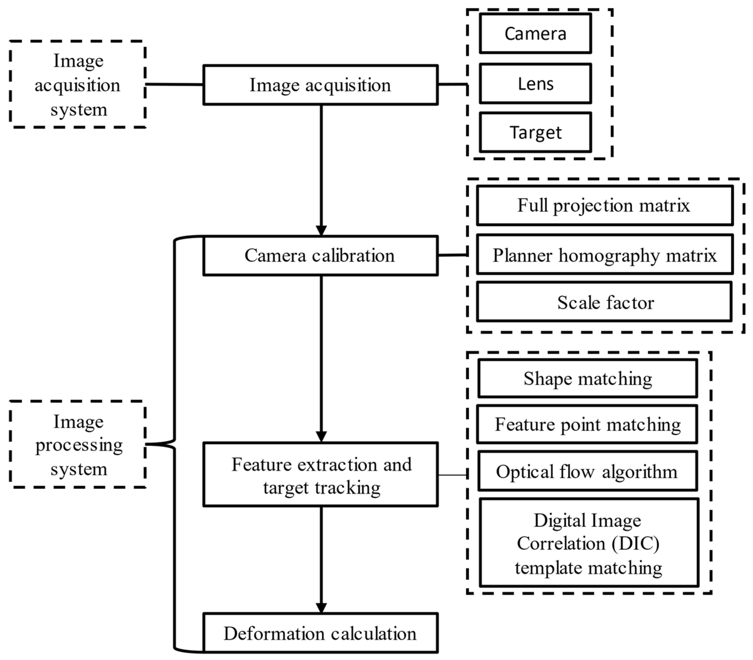
3. Basic Process
3.1. Image Acquisition
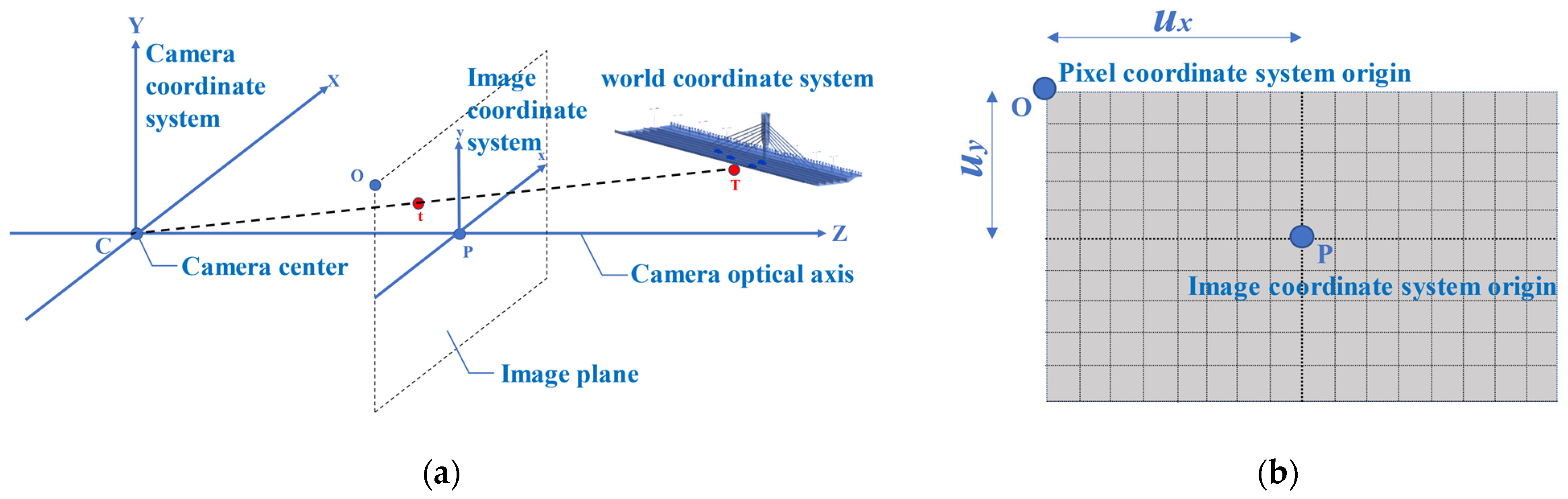
3.2. Camera Calibration
3.2.1. Full Projection Matrix
3.2.2. Planar Homography Matrix
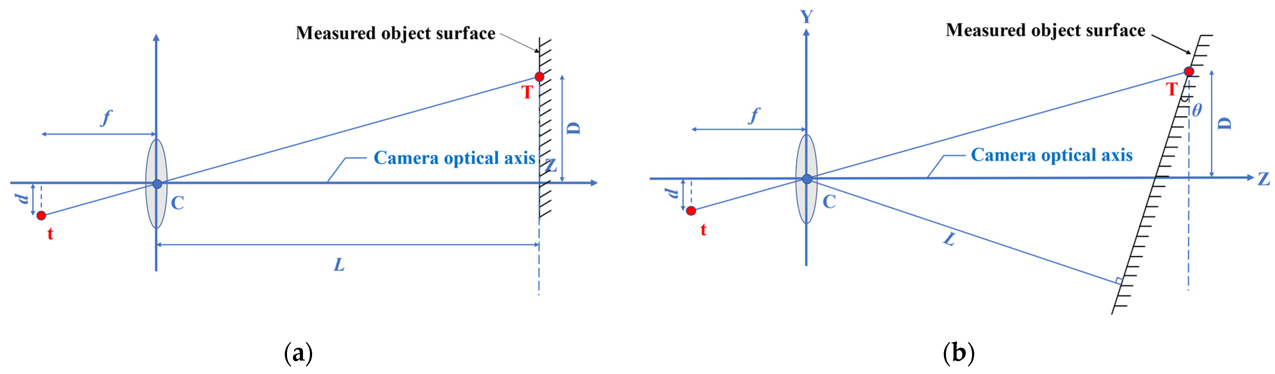
3.2.3. Scale Factor
3.3. Feature Extraction and Target Tracking
3.3.1. Shape Matching
3.3.2. Feature Point Matching
3.3.3. Optical Flow Algorithm
3.3.4. DIC Template Matching
3.4. Deformation Calculation
4. Computer Vision-Based Deformation Monitoring in Field Environment
4.1. Application Scenario of Computer Vision Monitoring System
4.2. Hardware Impact and Environmental Impact
4.2.1. Hardware Impact
- Camera
- Target
4.2.2. Environmental Impact
- Optical refraction
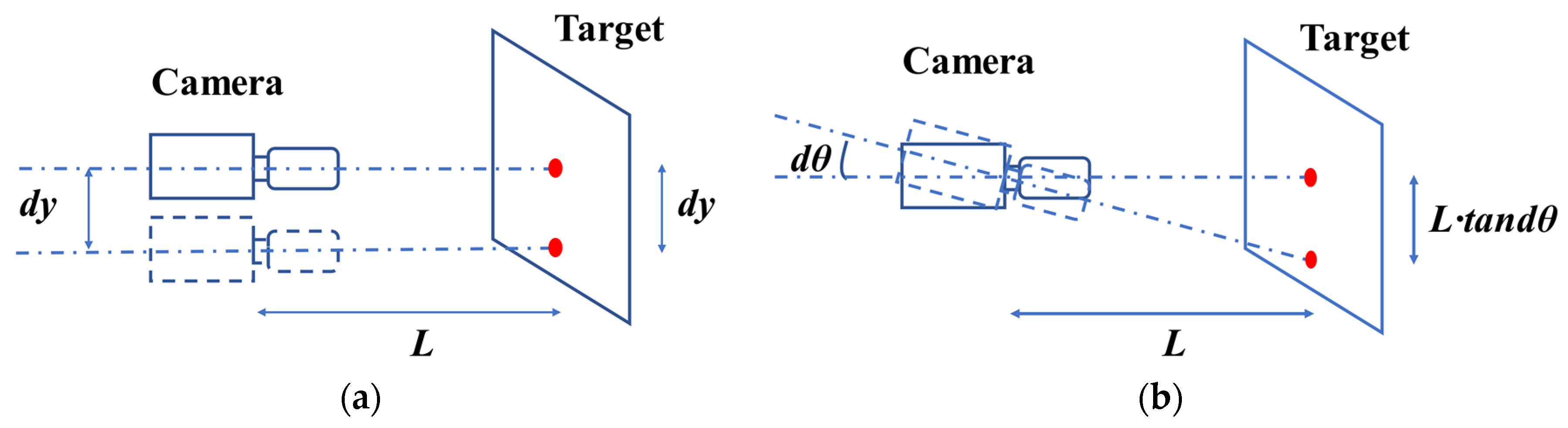
- Camera motion
- Illumination changes and partial occlusion
4.3. Impact of Target Tracking Algorithm
4.3.1. Image Preprocessing
4.3.2. Measurement Efficiency
4.3.3. Measurement Accuracy
4.3.4. Suggestions for Field Application Algorithms
4.4. Measurement Results
4.5. Other Impacts
5. Conclusions and Prospects
- (1)
- At present, the main application of computer vision in the field of SHM is still focused on the measurement of displacement time history curves of scale models under static and dynamic loading in controlled conditions and for short terms.
- (2)
- A large number of experimental tests and short-term field tests promote the formation of the basic framework of computer vision deformation monitoring systems, and existing research has focused on improving the applicability and stability of image processing algorithms.
- (3)
- Structural deformation monitoring systems based on computer vision have had some solutions to cope with individual external influences (such as target installation difficulty, illuminate change, camera movement and climate transformation). The accuracy and reliability of computer vision-based structural deformation monitoring has made great progress and is gradually approaching practical long-term monitoring.
Author Contributions
Funding
Data Availability Statement
Conflicts of Interest
References
- Feng, D.M.; Feng, M.Q.; Ozer, E.; Fukuda, Y. A vision-based sensor for noncontact structural displacement measurement. Sensors 2015, 15, 16557–16575. [Google Scholar] [CrossRef] [PubMed]
- Fukuda, Y.; Feng, M.Q.; Shinozuka, M. Cost-effective vision-based system for monitoring dynamic response of civil engineering structures. Struct. Control Health Monit. 2010, 17, 918–936. [Google Scholar] [CrossRef]
- Feng, D.M.; Feng, M.Q. Computer vision for SHM of civil infrastructure: From dynamic response measurement to damage detection—A review. Eng. Struct. 2018, 156, 105–117. [Google Scholar] [CrossRef]
- Bastianini, F.; Corradi, M.; Borri, A.; Tommaso, A.D. Retrofit and monitoring of an historical building using “Smart” CFRP with embedded fibre optic Brillouin sensors. Constr. Build. Mater. 2005, 19, 525–535. [Google Scholar] [CrossRef]
- Chan, T.H.T.; Yu, L.; Tam, H.Y.; Ni, Y.-Q.; Liu, S.Y.; Chung, W.H.; Cheng, L.K. Fiber Bragg grating sensors for structural health monitoring of Tsing Ma bridge: Background and experimental observation. Eng. Struct. 2006, 28, 648–659. [Google Scholar] [CrossRef]
- He, J.; Zhou, Z.; Jinping, O. Optic fiber sensor-based smart bridge cable with functionality of self-sensing. Mech. Syst. Signal Process. 2013, 35, 84–94. [Google Scholar] [CrossRef]
- Li, H.; Ou, J.; Zhou, Z. Applications of optical fibre Bragg gratings sensing technology-based smart stay cables. Opt. Lasers Eng. 2009, 47, 1077–1084. [Google Scholar] [CrossRef]
- Metje, N.; Chapman, D.; Rogers, C.; Henderson, P.; Beth, M. An Optical Fiber Sensor System for Remote Displacement Monitoring of Structures—Prototype Tests in the Laboratory. Struct. Health Monit. 2008, 7, 51–63. [Google Scholar] [CrossRef]
- Rodrigues, C.; Cavadas, F.; Félix, C.; Figueiras, J. FBG based strain monitoring in the rehabilitation of a centenary metallic bridge. Eng. Struct. 2012, 44, 281–290. [Google Scholar] [CrossRef]
- Hester, D.; Brownjohn, J.; Bocian, M.; Xu, Y. Low cost bridge load test: Calculating bridge displacement from acceleration for load assessment calculations. Eng. Struct. 2017, 143, 358–374. [Google Scholar] [CrossRef]
- Gindy, M.; Nassif, H.H.; Velde, J. Bridge Displacement Estimates from Measured Acceleration Records. Transp. Res. Rec. J. Transp. Res. Board 2007, 2028, 136–145. [Google Scholar] [CrossRef]
- Çelebi, M. GPS in dynamic monitoring of long-period structures. Soil Dyn. Earthq. Eng. 2000, 20, 477–483. [Google Scholar] [CrossRef]
- Nakamura, S.-I. GPS Measurement of Wind-Induced Suspension Bridge Girder Displacements. J. Struct. Eng. 2000, 126, 1413–1419. [Google Scholar] [CrossRef]
- Xu, L.; Guo, J.J.; Jiang, J.J. Time–frequency analysis of a suspension bridge based on GPS. J. Sound Vib. 2002, 254, 105–116. [Google Scholar] [CrossRef]
- Garg, P.; Moreu, F.; Ozdagli, A.; Taha, M.R.; Mascareñas, D. Noncontact Dynamic Displacement Measurement of Structures Using a Moving Laser Doppler Vibrometer. J. Bridg. Eng. 2019, 24, 04019089. [Google Scholar] [CrossRef]
- Teskey, R.S.; Radovanovic, W.F. Dynamic monitoring of deforming structures: Gps versus robotic tacheometry systems. In Proceedings of the International Symposium on Deformation Measurements, Orange, CA, USA, 19–22 March 2001. [Google Scholar]
- Pieraccini, M.; Parrini, F.; Fratini, M.; Atzeni, C.; Spinelli, P.; Micheloni, M. Static and dynamic testing of bridges through microwave interferometry. NDT E Int. 2007, 40, 208–214. [Google Scholar] [CrossRef]
- Chang, C.-C.; Xiao, X.H. Three-Dimensional Structural Translation and Rotation Measurement Using Monocular Videogrammetry. J. Eng. Mech. 2010, 136, 840–848. [Google Scholar] [CrossRef]
- Fukuda, Y.; Feng, M.Q.; Narita, Y.; Kaneko, S.; Tanaka, T. Vision-based displacement sensor for monitoring dynamic response using robust object search algorithm. IEEE Sens. J. 2013, 13, 4725–4732. [Google Scholar] [CrossRef]
- Kohut, P.; Holak, K.; Uhl, T.; Ortyl, Ł.; Owerko, T.; Kuras, P.; Kocierz, R. Monitoring of a civil structure’s state based on noncontact measurements. Struct. Health Monit. 2013, 12, 411–429. [Google Scholar] [CrossRef]
- Ribeiro, D.; Calçada, R.; Ferreira, J.; Martins, T. Non-contact measurement of the dynamic displacement of railway bridges using an advanced video-based system. Eng. Struct. 2014, 75, 164–180. [Google Scholar] [CrossRef]
- Casciati, F.; Fuggini, C. Monitoring a steel building using GPS sensors. Smart Struct. Syst. 2011, 7, 349–363. [Google Scholar] [CrossRef]
- Xu, Y.; Brownjohn, J.M.W.; Hester, D.; Koo, K.Y. Long-span bridges: Enhanced data fusion of GPS displacement and deck accelerations. Eng. Struct. 2017, 147, 639–651. [Google Scholar] [CrossRef]
- Mehrabi, A.B. In-Service Evaluation of Cable-Stayed Bridges, Overview of Available Methods and Findings. J. Bridg. Eng. 2006, 11, 716–724. [Google Scholar] [CrossRef]
- Nassif, H.H.; Gindy, M.; Davis, J. Comparison of laser Doppler vibrometer with contact sensors for monitoring bridge deflection and vibration. NDT E Int. 2005, 38, 213–218. [Google Scholar] [CrossRef]
- Casciati, F.; Wu, L.J. Local positioning accuracy of laser sensors for structural health monitoring. Struct. Control Health Monit. 2012, 20, 728–739. [Google Scholar] [CrossRef]
- Dong, C.Z.; Bas, S.; Catbas, N. A completely non-contact recognition system for bridge unit influence line using portable cameras and computer vision. Smart Struct Syst. 2019, 24, 617–630. [Google Scholar]
- Zaurin, R.; Catbas, F.N. Structural health monitoring using video stream, influence lines, and statistical analysis. Struct. Health Monit. 2010, 10, 309–332. [Google Scholar] [CrossRef]
- Khuc, T.; Catbas, F.N. Structural Identification Using Computer Vision–Based Bridge Health Monitoring. J. Struct. Eng. 2018, 144, 04017202. [Google Scholar] [CrossRef]
- Zhang, L.H.; Jin, Y.J.; Lin, L.; Li, J.J.; Du, Y.A. The comparison of ccd and cmos image sensors. In Proceedings of the International Conference on Optical Instruments and Technology—Advanced Sensor Technologies and Applications, Beijing, China, 16–19 November 2009. [Google Scholar]
- Bigas, M.; Cabruja, E.; Forest, J.; Salvi, J. Review of CMOS image sensors. Microelectron. J. 2006, 37, 433–451. [Google Scholar] [CrossRef]
- Khuc, T.; Catbas, F.N. Computer vision-based displacement and vibration monitoring without using physical target on structures. Struct. Infrastruct. Eng. 2017, 13, 505–516. [Google Scholar] [CrossRef]
- Lee, J.; Lee, K.-C.; Cho, S.; Sim, S.-H. Computer Vision-Based Structural Displacement Measurement Robust to Light-Induced Image Degradation for In-Service Bridges. Sensors 2017, 17, 2317. [Google Scholar] [CrossRef] [PubMed]
- Lee, J.-H.; Ho, H.-N.; Shinozuka, M.; Lee, J.-J. An advanced vision-based system for real-time displacement measurement of high-rise buildings. Smart Mater. Struct. 2012, 21, 125019. [Google Scholar] [CrossRef]
- Ye, X.; Dong, C. Review of computer vision-based structural displacement monitoring. China J. Highw. Transp. 2019, 32, 21–39. [Google Scholar]
- Ji, Y.F. A computer vision-based approach for structural displacement measurement. In Proceedings of the Conference on Sensors and Smart Structures Technologies for Civil, Mechanical, and Aerospace Systems 2010, San Diego, CA, USA, 7–11 March 2010; Spie-Int Soc Optical Engineering: Bellingham, DC, USA, 2010. [Google Scholar]
- Shariati, A.; Schumacher, T. Eulerian-based virtual visual sensors to measure dynamic displacements of structures. Struct. Control Health Monit. 2017, 24, e1977. [Google Scholar] [CrossRef]
- Yoon, H.; Elanwar, H.; Choi, H.; Golparvar-Fard, M.; Spencer, B.F., Jr. Target-free approach for vision-based structural system identification using consumer-grade cameras. Struct. Control Health Monit. 2016, 23, 1405–1416. [Google Scholar] [CrossRef]
- Kuddus, M.A.; Li, J.; Hao, H.; Li, C.; Bi, K. Target-free vision-based technique for vibration measurements of structures subjected to out-of-plane movements. Eng. Struct. 2019, 190, 210–222. [Google Scholar] [CrossRef]
- Lepetit, V.; Fua, P. Monocular Model-Based 3D Tracking of Rigid Objects: A Survey. Found. Trends Comput. Graph. Vis. 2005, 1, 89. [Google Scholar] [CrossRef]
- Chang, C.-C.; Ji, Y.F. Flexible Videogrammetric Technique for Three-Dimensional Structural Vibration Measurement. J. Eng. Mech. 2007, 133, 656–664. [Google Scholar] [CrossRef]
- Dong, C.-Z.; Catbas, F.N. A non-target structural displacement measurement method using advanced feature matching strategy. Adv. Struct. Eng. 2019, 22, 3461–3472. [Google Scholar] [CrossRef]
- Zhang, Z. A flexible new technique for camera calibration. IEEE Trans. Pattern Anal. Mach. Intell. 2000, 22, 1330–1334. [Google Scholar] [CrossRef]
- Heikkila, J. Geometric camera calibration using circular control points. IEEE Trans. Pattern Anal. Mach. Intell. 2000, 22, 1066–1077. [Google Scholar] [CrossRef]
- Fleet, D.J.; Jepson, A.D. Computation of component image velocity from local phase information. Int. J. Comput. Vis. 1990, 5, 77–104. [Google Scholar] [CrossRef]
- Sturm, P.F.; Maybank, S.J. On plane-based camera calibration: A general algorithm, singularities, applications. In Proceedings of the 1999 IEEE Computer Society Conference on Computer Vision and Pattern Recognition (CVPR’99), Fort Collins, CO, USA, 23–25 June 1999; IEEE: Piscataway, NJ, USA, 1999. [Google Scholar]
- Xu, Y.; Zhang, J.; Brownjohn, J. An accurate and distraction-free vision-based structural displacement measurement method integrating Siamese network based tracker and correlation-based template matching. Measurement 2021, 179, 109506. [Google Scholar] [CrossRef]
- Xu, Y.; Brownjohn, J.M.W.; Hester, D.; Koo, K.-Y. Dynamic displacement measurement of a long-span bridge using vision-based system. In Proceedings of the 8th European Workshop on Structural Health Monitoring, EWSHM 2016, Bilbao, Spain, 5–8 July 2016. [Google Scholar]
- Ye, X.W.; Yi, T.-H.; Dong, C.Z.; Liu, T. Vision-based structural displacement measurement: System performance evaluation and influence factor analysis. Measurement 2016, 88, 372–384. [Google Scholar] [CrossRef]
- Ye, X.W.; Jin, T.; Ang, P.-P.; Bian, X.-C.; Chen, Y.-M. Computer vision-based monitoring of the 3-d structural deformation of an ancient structure induced by shield tunneling construction. Struct. Control Health Monit. 2021, 28, e2702. [Google Scholar] [CrossRef]
- Feng, D.; Feng, M.Q. Experimental validation of cost-effective vision-based structural health monitoring. Mech. Syst. Signal Process. 2017, 88, 199–211. [Google Scholar] [CrossRef]
- Song, Y.-Z.; Bowen, C.R.; Kim, A.H.; Nassehi, A.; Padget, J.; Gathercole, N. Virtual visual sensors and their application in structural health monitoring. Struct. Health Monit. 2014, 13, 251–264. [Google Scholar] [CrossRef]
- Ye, X.W.; Ni, Y.-Q.; Wai, T.; Wong, K.; Zhang, X.; Xu, F. A vision-based system for dynamic displacement measurement of long-span bridges: Algorithm and verification. Smart Struct. Syst. 2013, 12, 363–379. [Google Scholar] [CrossRef]
- Wahbeh, A.M.; Caffrey, J.P.; Masri, S.F. A vision-based approach for the direct measurement of displacements in vibrating systems. Smart Mater. Struct. 2003, 12, 785–794. [Google Scholar] [CrossRef]
- Ji, Y.F.; Chang, C.C. Nontarget Image-Based Technique for Small Cable Vibration Measurement. J. Bridg. Eng. 2008, 13, 34–42. [Google Scholar] [CrossRef]
- Ghosal, S.; Mehrotra, R. Orthogonal moment operators for subpixel edge detection. Pattern Recognit. 1993, 26, 295–306. [Google Scholar] [CrossRef]
- Sobel, I. Neighborhood coding of binary images for fast contour following and general binary array processing. Comput. Graph. Image Process. 1978, 8, 127–135. [Google Scholar] [CrossRef]
- Marr, D.; Hildreth, E. Theory of edge detection. Proc. R. Soc. Lond. Ser. B Biol. Sci. 1980, 207, 187–217. [Google Scholar]
- Canny, J. A computational approach to edge detection. IEEE Trans. Pattern Anal. Mach. Intell. 1986, 8, 679–698. [Google Scholar] [CrossRef]
- Ballard, D. Generalizing the Hough transform to detect arbitrary shapes. Pattern Recognit. 1981, 13, 111–122. [Google Scholar] [CrossRef]
- Ji, Y.F.; Chang, C.C. Nontarget Stereo Vision Technique for Spatiotemporal Response Measurement of Line-Like Structures. J. Eng. Mech. 2008, 134, 466–474. [Google Scholar] [CrossRef]
- Tian, Y.D.; Zhang, J.; Yu, S.S. Vision-based structural scaling factor and flexibility identification through mobile impact testing. Mech. Syst. Signal Process. 2019, 122, 387–402. [Google Scholar] [CrossRef]
- Xu, Y.; Brownjohn, J.; Kong, D. A non-contact vision-based system for multipoint displacement monitoring in a cable-stayed footbridge. Struct. Control Health Monit. 2018, 25, e2155. [Google Scholar] [CrossRef]
- Khuc, T.; Catbas, F.N. Completely contactless structural health monitoring of real-life structures using cameras and computer vision. Struct. Control Health Monit. 2017, 24, e1852. [Google Scholar] [CrossRef]
- Harris, C.G.; Stephens, M. A Combined Corner and Edge Detector. In Proceedings of the Alvey Vision Conference, Manchester, UK, 31 August–2 September 1988. [Google Scholar] [CrossRef]
- Jianbo, S.; Tomasi, C. Good features to track. In Proceedings of the 1994 IEEE Computer Society Conference on Computer Vision and Pattern Recognition (Cat No94CH3405-8), Seattle, WA, USA, 21–23 June 1994; pp. 593–600. [Google Scholar]
- Gao, K.; Lin, S.X.; Zhang, Y.D.; Tang, S.; Ren, H.M. Attention model based sift keypoints filtration for image retrieval. In Proceedings of the 7th IEEE/ACIS International Conference on Computer and Information Science in Conjunction with 2nd IEEE/ACIS International Workshop on e-Activity, Portland, OR, USA, 14–16 May 2008. [Google Scholar]
- Bay, H.; Tuytelaars, T.; Van Gool, L. Surf: Speeded up robust features. In Computer Vision—ECCV 2006, Proceedings of the 9th European Conference on Computer Vision, Graz, Austria, 7–13 May 2006; Leonardis, A., Bischof, H., Pinz, A., Eds.; Springer: Berlin/Heidelberg, Germany, 2006; pp. 404–417. [Google Scholar]
- Calonder, M.; Lepetit, V.; Strecha, C.; Fua, P. Brief: Binary robust independent elementary features. In Computer Vision—ECCV 2010, Proceedings of the 11th European Conference on Computer Vision, Crete, Greece, 5–11 September 2010; Springer: Berlin/Heidelberg, Germany, 2010; pp. 778–792. [Google Scholar]
- Leutenegger, S.; Chli, M.; Siegwart, R.Y. Brisk: Binary robust invariant scalable keypoints. In Proceedings of the IEEE International Conference on Computer Vision (ICCV), Barcelona, Spain, 6–13 November 2011. [Google Scholar]
- Alahi, A.; Ortiz, R.; Vandergheynst, P. Freak: Fast retina keypoint. 2012 ieee conference on computer vision and pattern recognition. In Proceedings of the IEEE Conference on Computer Vision and Pattern Recognition, Providence, RI, USA, 16–21 June 2012; IEEE: New York, NY, USA, 2012; pp. 510–517. [Google Scholar]
- Dong, C.-Z.; Catbas, F.N. A review of computer vision–based structural health monitoring at local and global levels. Struct. Health Monit. 2020, 20, 692–743. [Google Scholar] [CrossRef]
- Sun, D.Q.; Roth, S.; Black, M.J. Secrets of optical flow estimation and their principles. In Proceedings of the 2010 IEEE Conference on Computer Vision and Pattern Recognition, Los Alamitos, CA, USA, 13–18 June 2010; pp. 2432–2439. [Google Scholar]
- Dong, C.-Z.; Celik, O.; Catbas, F.N. Marker-free monitoring of the grandstand structures and modal identification using computer vision methods. Struct. Health Monit. 2019, 18, 1491–1509. [Google Scholar] [CrossRef]
- Chen, Z.; Gao, M.; Shen, Y. The current situation and trends of optical flow estimation. J. Image Graph. 2002, 7, 434–439. [Google Scholar]
- Lucas, B.D.; Kanade, T. An iterative image registration technique with an application to stereo vision (darpa). In Proceedings of the 7th International Joint Conference on Artificial Intelligence, Vancouver, BC, Canada, 24–28 August 1981; pp. 674–679. [Google Scholar]
- Celik, O.; Dong, C.-Z.; Catbas, F.N. A computer vision approach for the load time history estimation of lively individuals and crowds. Comput. Struct. 2018, 200, 32–52. [Google Scholar] [CrossRef]
- Horn, B.K.; Schunck, B.G. Determining optical flow. Artif. Intell. 1981, 17, 185–203. [Google Scholar] [CrossRef]
- Farneback, G. Two-frame motion estimation based on polynomial expansion. In Image Analysis, Proceedings of the 13th Scandinavian Conference, SCIA 2003 Halmstad, Sweden, 29 June–2 July 2003; Lecture Notes in Computer Science; Bigun, J., Gustavsson, T., Eds.; Springer: Berlin/Heidelberg, Germany, 2003; pp. 363–370. [Google Scholar]
- Liu, B.; Zaccarin, A. New fast algorithms for the estimation of block motion vectors. IEEE Trans. Circuits Syst. Video Technol. 1993, 3, 148–157. [Google Scholar] [CrossRef]
- Wadhwa, N.; Rubinstein, M.; Durand, F.; Freeman, W.T. Phase-based video motion processing. ACM Trans. Graph. 2013, 32, 80. [Google Scholar] [CrossRef]
- Chen, J.G.; Wadhwa, N.; Cha, Y.-J.; Durand, F.; Freeman, W.T.; Buyukozturk, O. Modal identification of simple structures with high-speed video using motion magnification. J. Sound Vib. 2015, 345, 58–71. [Google Scholar] [CrossRef]
- Kim, S.W.; Jeon, B.-G.; Cheung, J.-H.; Kim, S.-D.; Park, J.-B. Stay cable tension estimation using a vision-based monitoring system under various weather conditions. J. Civ. Struct. Health Monit. 2017, 7, 343–357. [Google Scholar] [CrossRef]
- Pan, B.; Qian, K.M.; Xie, H.M.; Asundi, A. Two-dimensional digital image correlation for in-plane displacement and strain measurement: A review. Meas. Sci. Technol. 2009, 20, 17. [Google Scholar] [CrossRef]
- Fayyad, T.M.; Lees, J.M. Experimental investigation of crack propagation and crack branching in lightly reinforced concrete beams using digital image correlation. Eng. Fract. Mech. 2017, 182, 487–505. [Google Scholar] [CrossRef]
- Ghiassi, B.; Xavier, J.; Oliveira, D.V.; Lourenço, P.B. Application of digital image correlation in investigating the bond between FRP and masonry. Compos. Struct. 2013, 106, 340–349. [Google Scholar] [CrossRef]
- Guizar-Sicairos, M.; Thurman, S.T.; Fienup, J.R. Efficient subpixel image registration algorithms. Opt. Lett. 2008, 33, 156–158. [Google Scholar] [CrossRef] [PubMed]
- Swain, M.J.; Ballard, D.H. Color indexing. Int. J. Comput. Vis. 1991, 7, 11–32. [Google Scholar] [CrossRef]
- Jing, H.; Kumar, S.R.; Mitra, M.; Wei-Jing, Z.; Zabih, R. Image indexing using color correlograms. In Proceedings of the 1997 IEEE Computer Society Conference on Computer Vision and Pattern Recognition (Cat No97CB36082), San Juan, PR, USA, 17–19 June 1997; pp. 762–768. [Google Scholar]
- Cigada, A.; Mazzoleni, P.; Zappa, E. Vibration Monitoring of Multiple Bridge Points by Means of a Unique Vision-Based Measuring System. Exp. Mech. 2014, 54, 255–271. [Google Scholar] [CrossRef]
- Stephen, G.A.; Brownjohn, J.M.W.; Taylor, C.A. Measurements of static and dynamic displacement from visual monitoring of the Humber Bridge. Eng. Struct. 1993, 15, 197–208. [Google Scholar] [CrossRef]
- Macdonald, J.H.G.; Dagless, E.L.; Thomas, B.T.; Taylor, C.A. Dynamic measurements of the second severn crossing. Proc. Inst. Civ. Eng. Transp. 1997, 123, 241–248. [Google Scholar] [CrossRef]
- Tian, L.; Pan, B. Remote Bridge Deflection Measurement Using an Advanced Video Deflectometer and Actively Illuminated LED Targets. Sensors 2016, 16, 1344. [Google Scholar] [CrossRef]
- Kim, H.; Shin, S. Reliability verification of a vision-based dynamic displacement measurement for system identification. J. Wind Eng. Ind. Aerodyn. 2019, 191, 22–31. [Google Scholar] [CrossRef]
- Dong, C.Z.; Ye, X.W.; Jin, T. Identification of structural dynamic characteristics based on machine vision technology. Measurement 2018, 126, 405–416. [Google Scholar] [CrossRef]
- Lee, J.J.; Shinozuka, M. A vision-based system for remote sensing of bridge displacement. NDT E Int. 2006, 39, 425–431. [Google Scholar] [CrossRef]
- Ramana, L.; Choi, W.; Cha, Y.-J. Fully automated vision-based loosened bolt detection using the Viola–Jones algorithm. Struct. Health Monit. 2018, 18, 422–434. [Google Scholar] [CrossRef]
- Sun, J.H.; Xie, Y.X.; Cheng, X.Q. A Fast Bolt-Loosening Detection Method of Running Train’s Key Components Based on Binocular Vision. IEEE Access 2019, 7, 32227–32239. [Google Scholar] [CrossRef]
- Wang, C.Y.; Wang, N.; Ho, S.-C.; Chen, X.M.; Song, G.B. Design of a New Vision-Based Method for the Bolts Looseness Detection in Flange Connections. IEEE Trans. Ind. Electron. 2020, 67, 1366–1375. [Google Scholar] [CrossRef]
- Cha, Y.-J.; Choi, W.; Suh, G.; Mahmoudkhani, S.; Büyüköztürk, O. Autonomous Structural Visual Inspection Using Region-Based Deep Learning for Detecting Multiple Damage Types. Comput. Civ. Infrastruct. Eng. 2017, 33, 731–747. [Google Scholar] [CrossRef]
- Pan, X.; Yang, T.Y. Postdisaster image-based damage detection and repair cost estimation of reinforced concrete buildings using dual convolutional neural networks. Comput. Civ. Infrastruct. Eng. 2020, 35, 495–510. [Google Scholar] [CrossRef]
- Liang, X. Image-based post-disaster inspection of reinforced concrete bridge systems using deep learning with Bayesian optimization. Comput. Civ. Infrastruct. Eng. 2019, 34, 415–430. [Google Scholar] [CrossRef]
- Muhammad, K.; Ahmad, J.; Lv, Z.; Bellavista, P.; Yang, P.; Baik, S.W. Efficient Deep CNN-Based Fire Detection and Localization in Video Surveillance Applications. IEEE Trans. Syst. Man Cybern. Syst. 2018, 49, 1419–1434. [Google Scholar] [CrossRef]
- He, Y.; Zhang, L.; Chen, Z.; Li, C.Y. A framework of structural damage detection for civil structures using a combined multi-scale convolutional neural network and echo state network. Eng. Comput. 2022, 1–19. [Google Scholar] [CrossRef]
- Kim, S.W.; Kim, N.-S. Dynamic characteristics of suspension bridge hanger cables using digital image processing. NDT E Int. 2013, 59, 25–33. [Google Scholar] [CrossRef]
- Kim, S.W.; Jeon, B.-G.; Kim, N.-S.; Park, J.-C. Vision-based monitoring system for evaluating cable tensile forces on a cable-stayed bridge. Struct. Health Monit. 2013, 12, 440–456. [Google Scholar] [CrossRef]
- Ye, X.W.; Dong, C.Z.; Liu, T. Force monitoring of steel cables using vision-based sensing technology: Methodology and experimental verification. Smart Struct. Syst. 2016, 18, 585–599. [Google Scholar] [CrossRef]
- Chen, C.-C.; Wu, W.-H.; Tseng, H.-Z.; Chen, C.-H.; Lai, G.L. Application of digital photogrammetry techniques in identifying the mode shape ratios of stay cables with multiple camcorders. Measurement 2015, 75, 134–146. [Google Scholar] [CrossRef]
- Park, J.-W.; Lee, J.-J.; Jung, H.-J.; Myung, H. Vision-based displacement measurement method for high-rise building structures using partitioning approach. NDT E Int. 2010, 43, 642–647. [Google Scholar] [CrossRef]
- Feng, D.; Scarangello, T.; Feng, M.Q.; Ye, Q. Cable tension force estimate using novel noncontact vision-based sensor. Measurement 2017, 99, 44–52. [Google Scholar] [CrossRef]
- Feng, M.Q.; Fukuda, Y.; Feng, D.; Mizuta, M. Nontarget Vision Sensor for Remote Measurement of Bridge Dynamic Response. J. Bridge Eng. 2015, 20, 04015023. [Google Scholar] [CrossRef]
- Brownjohn, J.M.W.; Xu, Y.; Hester, D. Vision-Based Bridge Deformation Monitoring. Front. Built Environ. 2017, 3, 23. [Google Scholar] [CrossRef]
- Li, J.-C.; Yuan, B.-Z. Using vision technique for the bridge deformation detection. In Proceedings of the ICASSP ‘88: 1988 International Conference on Acoustics, Speech, and Signal Processing, New York, NY, USA, 11–14 April 1988; IEEE: New York, NY, USA, 1988. [Google Scholar]
- Feng, D.; Feng, M.Q. Vision-based multipoint displacement measurement for structural health monitoring. Struct. Control Health Monit. 2016, 23, 876–890. [Google Scholar] [CrossRef]
- Feng, D.; Feng, M.Q. Model Updating of Railway Bridge Using In Situ Dynamic Displacement Measurement under Trainloads. J. Bridg. Eng. 2015, 20, 04015019. [Google Scholar] [CrossRef]
- Lee, J.-J.; Ho, H.-N.; Lee, J.H. A Vision-Based Dynamic Rotational Angle Measurement System for Large Civil Structures. Sensors 2012, 12, 7326–7336. [Google Scholar] [CrossRef]
- Chen, Z.C.; Li, H.; Bao, Y.Q.; Li, N.; Jin, Y. Identification of spatio-temporal distribution of vehicle loads on long-span bridges using computer vision technology. Struct. Control Health Monit. 2016, 23, 517–534. [Google Scholar] [CrossRef]
- Yoon, H.; Shin, J.; Spencer, B.F. Structural Displacement Measurement Using an Unmanned Aerial System. Comput. Civ. Infrastruct. Eng. 2018, 33, 183–192. [Google Scholar] [CrossRef]
- Ma, S.P.; Pang, J.Z.; Ma, Q.W. The systematic error in digital image correlation induced by self-heating of a digital camera. Meas. Sci. Technol. 2012, 23, 7. [Google Scholar] [CrossRef]
- Ehrhart, M.; Lienhart, W. Image-based dynamic deformation monitoring of civil engineering structures from long ranges. In Image Processing: Machine Vision Applications viii. Proceedings of Spie. 9405; Lam, E.Y., Niel, K.S., Eds.; Spie-Int Soc Optical Engineering: Bellingham, DC, USA, 2015. [Google Scholar]
- Ye, X.W.; Yi, T.-H.; Dong, C.Z.; Liu, T.; Bai, H. Multi-point displacement monitoring of bridges using a vision-based approach. Wind Struct. Int. J. 2015, 20, 315–326. [Google Scholar] [CrossRef]
- Anantrasirichai, N.; Achim, A.; Kingsbury, N.G.; Bull, D.R. Atmospheric Turbulence Mitigation Using Complex Wavelet-Based Fusion. IEEE Trans. Image Process. 2013, 22, 2398–2408. [Google Scholar] [CrossRef]
- Shimizu, M.; Yoshimura, S.; Tanaka, M.; Okutomi, M. Super-resolution from image sequence under influence of hot-air optical turbulence. In Proceedings of the IEEE Conference on Computer Vision and Pattern Recognition, Anchorage, AK, USA, 23–28 June 2008. [Google Scholar]
- Zhu, X.; Milanfar, P. Removing Atmospheric Turbulence via Space-Invariant Deconvolution. IEEE Trans. Pattern Anal. Mach. Intell. 2012, 35, 157–170. [Google Scholar] [CrossRef]
- Luo, L.X.; Feng, M.Q.; Wu, J. A comprehensive alleviation technique for optical-turbulence-induced errors in vision-based displacement measurement. Struct. Control Health Monit. 2020, 27, 16. [Google Scholar] [CrossRef]
- Luo, L.X.; Feng, M.Q.; Wu, J.P.; Bi, L.Z. Modeling and Detection of Heat Haze in Computer Vision Based Displacement Measurement. Measurement 2021, 182, 109772. [Google Scholar] [CrossRef]
- Owens, J.C. Optical Refractive Index of Air: Dependence on Pressure, Temperature and Composition. Appl. Opt. 1967, 6, 51–59. [Google Scholar] [CrossRef]
- Yoneyama, S.; Ueda, H. Bridge Deflection Measurement Using Digital Image Correlation with Camera Movement Correction. Mater. Trans. 2012, 53, 285–290. [Google Scholar] [CrossRef]
- Hoskere, V.; Park, J.-W.; Yoon, H.; Spencer, B.F., Jr. Vision-Based Modal Survey of Civil Infrastructure Using Unmanned Aerial Vehicles. J. Struct. Eng. 2019, 145, 04019062. [Google Scholar] [CrossRef]
- Casciati, F.; Casciati, S.; Colnaghi, A.; Faravelli, L.; Rosadini, L.; Zhu, S. Vision-based support in the characterization of superelastic u-shaped sma elements. Smart Struct. Syst. 2019, 24, 641–648. [Google Scholar]
- Ribeiro, D.; Santos, R.; Cabral, R.; Saramago, G.; Montenegro, P.; Carvalho, H.; Correia, J.; Calçada, R. Non-contact structural displacement measurement using Unmanned Aerial Vehicles and video-based systems. Mech. Syst. Signal Process. 2021, 160, 107869. [Google Scholar] [CrossRef]
- Lee, J.; Lee, K.-C.; Jeong, S.; Lee, Y.-J.; Sim, S.-H. Long-term displacement measurement of full-scale bridges using camera ego-motion compensation. Mech. Syst. Signal Process. 2020, 140, 106651. [Google Scholar] [CrossRef]
- Chen, J.G.; Davis, A.; Wadhwa, N.; Durand, F.; Freeman, W.T.; Büyüköztürk, O. Video Camera–Based Vibration Measurement for Civil Infrastructure Applications. J. Infrastruct. Syst. 2017, 23, 11. [Google Scholar] [CrossRef]
- Khaloo, A.; Lattanzi, D. Pixel-wise structural motion tracking from rectified repurposed videos. Struct. Control Health Monit. 2017, 24, e2009. [Google Scholar] [CrossRef]
- Rousseeuw, P.J.; Hubert, M. Robust statistics for outlier detection. Wiley Interdiscip. Rev-Data Min. Knowl. Discov. 2011, 1, 73–79. [Google Scholar] [CrossRef]
- Spencer, B.F., Jr.; Hoskere, V.; Narazaki, Y. Advances in Computer Vision-Based Civil Infrastructure Inspection and Monitoring. Engineering 2019, 5, 199–222. [Google Scholar] [CrossRef]
- Li, Y.; Takauji, H.; Ohmura, I.; Kaneko, S.; Tanaka, T. Robust Focusing using Orientation Code Matching. J. Jpn. Soc. Precis. Eng. 2009, 75, 650–656. [Google Scholar] [CrossRef][Green Version]
- Ullah, F.; Kaneko, S.; Igarashi, S. Orientation code matching for robust object search. IEICE Trans. Inf. Syst. 2001, E84D, 999–1006. [Google Scholar]
- Luo, L.; Feng, M.Q. Edge-Enhanced Matching for Gradient-Based Computer Vision Displacement Measurement. Comput. Civ. Infrastruct. Eng. 2018, 33, 1019–1040. [Google Scholar] [CrossRef]
- Luo, L.; Feng, M.Q.; Wu, Z.Y. Robust vision sensor for multi-point displacement monitoring of bridges in the field. Eng. Struct. 2018, 163, 255–266. [Google Scholar] [CrossRef]
- Lichao, Z.; Gonzalez-Garcia, A.; Van De Weijer, J.; Danelljan, M.; Khan, F.S. Learning the model update for siamese trackers. In Proceedings of the 2019 IEEE/CVF International Conference on Computer Vision (ICCV), Seoul, Korea, 27–28 October 2019; pp. 4009–4018. [Google Scholar]
- Dong, C.-Z.; Celik, O.; Catbas, F.N.; Obrien, E.; Taylor, S. A Robust Vision-Based Method for Displacement Measurement under Adverse Environmental Factors Using Spatio-Temporal Context Learning and Taylor Approximation. Sensors 2019, 19, 3197. [Google Scholar] [CrossRef] [PubMed]
- Javh, J.; Slavič, J.; Boltežar, M. High frequency modal identification on noisy high-speed camera data. Mech. Syst. Signal Process. 2018, 98, 344–351. [Google Scholar] [CrossRef]
- Lecompte, D.; Smits, A.; Bossuyt, S.; Sol, H.; Vantomme, J.; Van Hemelrijck, D.; Habraken, A.M. Quality assessment of speckle patterns for digital image correlation. Opt. Lasers Eng. 2006, 44, 1132–1145. [Google Scholar] [CrossRef]
- Zhang, D.; Guo, J.; Lei, X.; Zhu, C. A High-Speed Vision-Based Sensor for Dynamic Vibration Analysis Using Fast Motion Extraction Algorithms. Sensors 2016, 16, 572. [Google Scholar] [CrossRef]
- Guo, J.; Zhu, C. Dynamic displacement measurement of large-scale structures based on the Lucas–Kanade template tracking algorithm. Mech. Syst. Signal Process. 2016, 66–67, 425–436. [Google Scholar] [CrossRef]
- Pan, B.; Xie, H.M.; Xu, B.Q.; Dai, F.L. Performance of sub-pixel registration algorithms in digital image correlation. Meas Sci Technol. 2006, 17, 1615–1621. [Google Scholar]
- Macvicar-Whelan, P.J.; Binford, T.O. Line finding with subpixel precision. Proc. SPIE—Int. Soc. Opt. Eng. 1981, 281, 211–216. [Google Scholar]
- Jensen, K.; Anastassiou, D. Subpixel edge localization and the interpolation of still images. IEEE Trans. Image Process. 1995, 4, 285–295. [Google Scholar] [CrossRef]
- Bruck, H.A.; Mcneill, S.R.; Sutton, M.A.; Peters, W.H. Digital image correlation using newton-raphson method of partial differential correction displacement measurement. Exp. Mech. 1989, 29, 261–267. [Google Scholar] [CrossRef]
- Pan, B.; Li, K.; Tong, W. Fast, Robust and Accurate Digital Image Correlation Calculation Without Redundant Computations. Exp. Mech. 2013, 53, 1277–1289. [Google Scholar] [CrossRef]
- Qu, Y.D.; Cui, C.S.; Chen, S.B.; Li, J.Q. A fast subpixel edge detection method using sobel-zernike moments operator. Image Vis Comput. 2005, 23, 11–17. [Google Scholar]
- Mas, D.; Perez, J.; Ferrer, B.; Espinosa, J. Realistic limits for subpixel movement detection. Appl. Opt. 2016, 55, 4974–4979. [Google Scholar] [CrossRef] [PubMed]
- Khuc, T.; Nguyen, T.A.; Dao, H.; Catbas, F.N. Swaying displacement measurement for structural monitoring using computer vision and an unmanned aerial vehicle. Measurement 2020, 159, 107769. [Google Scholar] [CrossRef]
- Shan, B.H.; Zheng, S.J.; Ou, J.P. Free vibration monitoring experiment of a stayed-cable model based on stereovision. Measurement 2015, 76, 228–239. [Google Scholar] [CrossRef]
- Pan, B.; Li, K. A fast digital image correlation method for deformation measurement. Opt. Lasers Eng. 2011, 49, 841–847. [Google Scholar] [CrossRef]
- Xu, Y.; Brownjohn, J.M.W.; Huseynov, F. Accurate Deformation Monitoring on Bridge Structures Using a Cost-Effective Sensing System Combined with a Camera and Accelerometers: Case Study. J. Bridg. Eng. 2019, 24, 05018014. [Google Scholar] [CrossRef]
- Lee, J.J.; Shinozuka, M. Real-Time Displacement Measurement of a Flexible Bridge Using Digital Image Processing Techniques. Exp. Mech. 2006, 46, 105–114. [Google Scholar] [CrossRef]
- Lee, J.J.; Fukuda, Y.; Shinozuka, M.; Cho, S.; Yun, C.-B. Development and application of a vision-based displacement measurement system for structural health monitoring of civil structures. Smart Struct. Syst. 2007, 3, 373–384. [Google Scholar] [CrossRef]


| Algorithms | Characteristics and Restraints | Application Scenarios |
|---|---|---|
| Shape matching | High efficiency, real-time monitoring, robust properties to non-uniform illumination and partial edge blur, distinct geometry features; short-distance monitoring | Cable structure, tower, long-span bridge, stadium |
| Feature point matching | High efficiency, high accuracy, robust to illumination change, distinct geometry features; rich surface texture, uncertain number of feature points, short-distance monitoring | Stadium structure, footbridge, railway bridge, urban bridge |
| Optical flow algorithm | Full field displacement, natural target, suitable for motion tracking; short-distance monitoring, sensitive to illumination change and partial occlusion | Stadium structure, footbridge, railway bridge, urban bridge |
| DIC template matching | Long-distance and short-distance monitoring; artificial target, sensitive to illumination change | Cable structure, long-span bridge, stadium structure, footbridge, railway bridge, urban bridge, tower |
| Research Point | Reference | Algorithms | Test Description | Results |
|---|---|---|---|---|
| Target | Ehrhart et al. [120] (2015) | Shape matching (artificial target) | Shaking table test, least squares fit of ellipse, precision quantitative evaluation of accuracy | At the distance of 6 m and 31 m, the error is less than 0.01 mm and 0.2 mm, respectively |
| Tian et al. [93] (2016) | DIC template matching (artificial target) | Field test, DIC technology based on IC-GN, displacement~time history curve | At the distance of 300 m, the average error is 0.5674 mm | |
| Feng et al. [115] (2015) | Template matching (natural target) | Railway bridge test, modal identification, modify finite element model | At the distance of 9 m, the vision sensor and the accelerometer measure the exact same first-order frequency | |
| Khuc et al. [64] (2017) | Feature point matching (natural target) | Stadium grandstand structure test, feature extraction with Hessian matrix, dynamic displacement measurement | At the distance of 3 m and 13 m, the error is less than 0.01 mm and 0.04 mm, respectively | |
| Khuc et al. [154] (2020) | Feature point matching (natural target) | Tower test, Canny edge detection and Hough transform, modal identification | At the distance of 1.84 m, first-order natural frequency error below 2% | |
| Camera motion and optical refraction | Garg et al. [15] (2019) | Digital high-pass filtering | Shaking table test, dynamic displacement measurement | At the distance of 4 m, the maximum error is between 10~15%, and the RMS error is between 2~5% |
| Ye et al. [50] (2021) | Background modification | Long-term field monitoring, 3D structural deformation measurement | Eliminate the error caused by thermal expansion and cold contraction of camera bracket | |
| Lee et al. [132] (2020) | Ego-motion compensation | Long-term field monitoring, displacement measurement | Measurement error is reduced from 44.1 mm to 1.1 mm | |
| Ribeiro et al. [131] (2021) | Inertial measuring unit | Experiment test, modal identification, dynamic displacement measurement | The maximum error of displacement measurement is 1.47 mm and RMS error is 9.3% | |
| Luo et al. [125] (2020) | Adaptive optical-turbulence error filter | Field test, displacement~time history curve | Measurement errors are significantly reduced by about 67.5% from 0.0845 to 0.0275 mm | |
| Illumination change and partial occlusion | Ribeiro et al. [21] (2014) | Artificial light source | Field test, using artificial light source, displacement ~ time history curve | At the distance of 15 m and 25 m, the error is less than 0.1 mm and 0.25 mm, respectively |
| Feng et al. [111] (2015) | A matching algorithm based on the gradient information | Field test, a matching algorithm based on the gradient information, dynamic response of steel and concrete bridges under train load | At the distance of 30.48 m, the maximum displacement error is 2.83%, and the average error is 1.39% | |
| Shan et al. [155] (2015) | Shape matching | Cable force measurement, shape matching, cable modal identification | The first three frequencies of free vibration of stayed-cable model are accurately measured | |
| Dong et al. [142] (2019) | A matching method based on Spatio-Temporal Context Learning | Experiment test, a matching method based on Spatio-Temporal Context Learning, illumination change and fog interference, displacement~time history curve | The proposed subpixel estimation method is faster than UCC by about 50 times | |
| Xu et al. [47] (2021) | Combined with deep learning | Field test, displacement~time history curve | Centimeter-level accuracy can be achieved at distances of more than 715 m | |
| Image preprocessing | Kim et al. [105] (2013) | Image transform technology | Ambient vibration tests, suspension bridge hanger cables, dynamic response and modal frequencies | The error of measuring sling modal frequency and cable force is within 0.5% |
| Kim et al. [106] (2013) | Image enhancement techniques | Ambient vibration tests, smoothing filter and sharpening filter, stay cables, dynamic response | The error of measuring suspension bridge hanger cables natural frequency and cable force is within 2% | |
| Tian et al. [62] (2019) | Image description and segmentation technology | Impact test, Hough transform based on gradient, modal parameters identification | The recognition rate of vibration mode is more than 84% | |
| Measurement efficiency and accuracy | Qu et al. [152] (2005) | Edge detection method using Sobel-Zernike moments operator | numerical tests | The accuracy reaches 87.75% of the sub-pixel level, and the speed is increased by 5 times |
| Pan et al. [156] (2011) | DIC template matching based on Newton-Raphson algorithm | Experimental verification, full filed deformation measurement | Without any loss of measurement accuracy, the calculation speed is increased by 120~200 times | |
| Pan et al. [151] (2013) | DIC template matching based on IC-GN | Numerical tests and experimental verification | The proposed IC-GN is 3~5 times faster than Newton-Raphson | |
| Zhang et al. [145] (2016) | Integrate two efficient subpixel level motion extraction algorithms | Experimental verification, Taylor approximation refinement algorithm and the localization refinement algorithm, dynamic vibration analysis | In the case of similar accuracy, it is at least 5 times faster than the traditional UCC method (RMS error 0.75%) | |
| Xu et al. [157] (2019) | Fuse the vision-based displacement measurement with acceleration data | Field test, short-span railway bridge, displacement ~ time history curve | The RMS of measurement noise at the camera-to-target distance of 6.9 m is less than 0.2 mm |
Publisher’s Note: MDPI stays neutral with regard to jurisdictional claims in published maps and institutional affiliations. |
© 2022 by the authors. Licensee MDPI, Basel, Switzerland. This article is an open access article distributed under the terms and conditions of the Creative Commons Attribution (CC BY) license (https://creativecommons.org/licenses/by/4.0/).
Share and Cite
Zhuang, Y.; Chen, W.; Jin, T.; Chen, B.; Zhang, H.; Zhang, W. A Review of Computer Vision-Based Structural Deformation Monitoring in Field Environments. Sensors 2022, 22, 3789. https://doi.org/10.3390/s22103789
Zhuang Y, Chen W, Jin T, Chen B, Zhang H, Zhang W. A Review of Computer Vision-Based Structural Deformation Monitoring in Field Environments. Sensors. 2022; 22(10):3789. https://doi.org/10.3390/s22103789
Chicago/Turabian StyleZhuang, Yizhou, Weimin Chen, Tao Jin, Bin Chen, He Zhang, and Wen Zhang. 2022. "A Review of Computer Vision-Based Structural Deformation Monitoring in Field Environments" Sensors 22, no. 10: 3789. https://doi.org/10.3390/s22103789
APA StyleZhuang, Y., Chen, W., Jin, T., Chen, B., Zhang, H., & Zhang, W. (2022). A Review of Computer Vision-Based Structural Deformation Monitoring in Field Environments. Sensors, 22(10), 3789. https://doi.org/10.3390/s22103789