Performance Enhancement of Consumer-Grade MEMS Sensors through Geometrical Redundancy


Abstract
:1. Introduction
2. Theoretical Background
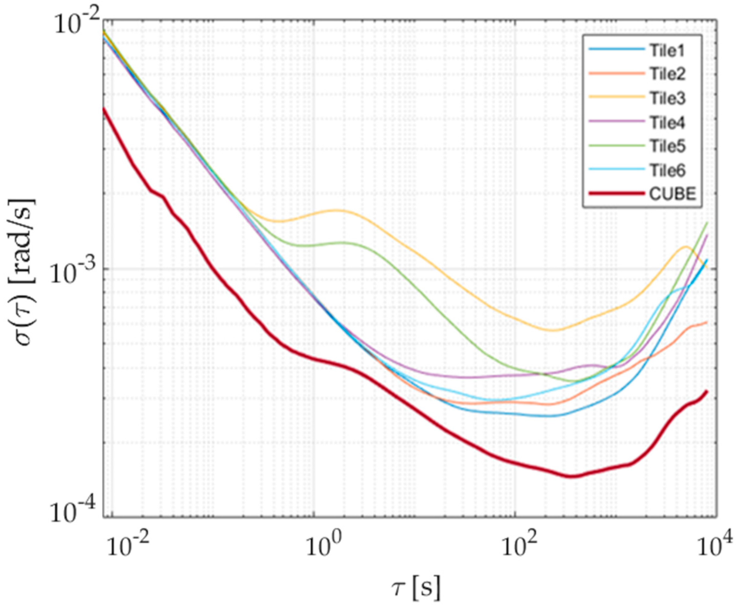
2.1. Advantages of Redundant Configuration
2.2. Sensing Axes Alignment
2.3. Kalman Filter
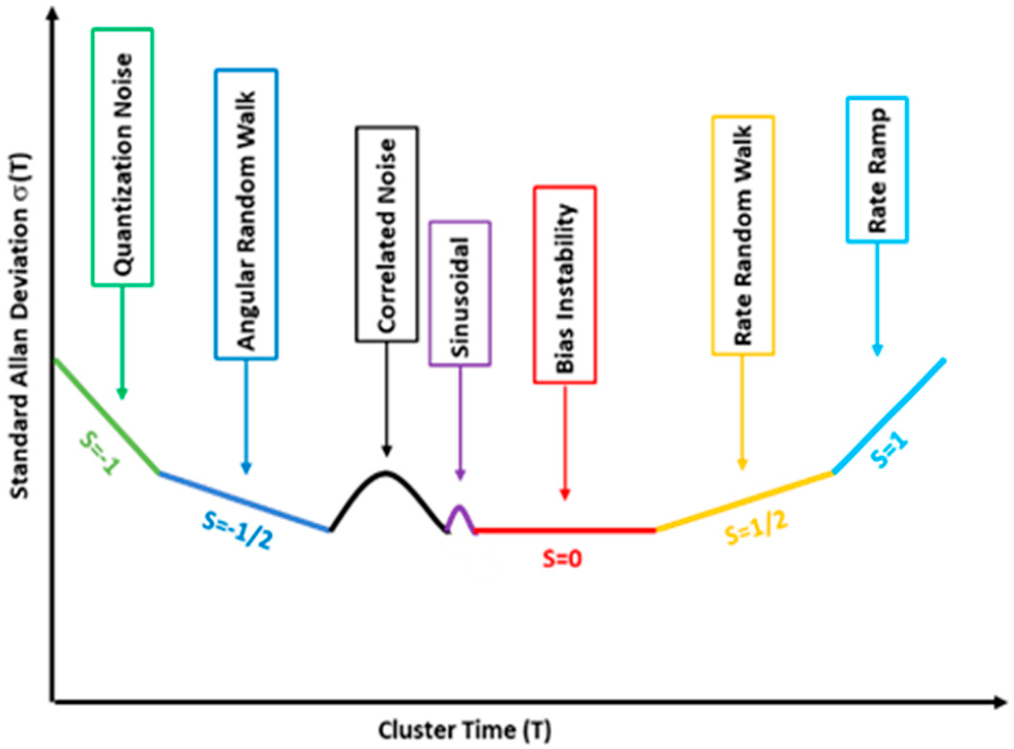
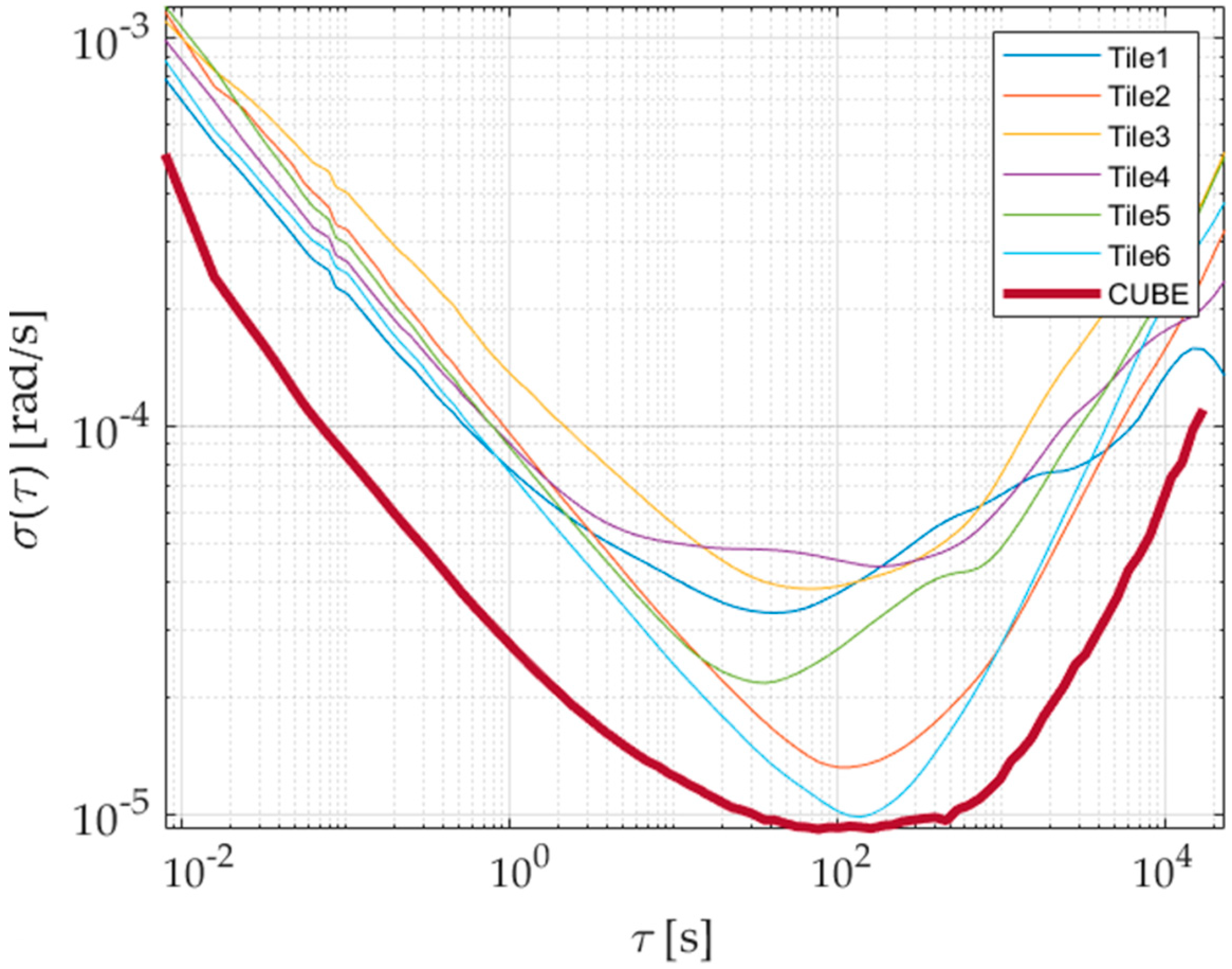
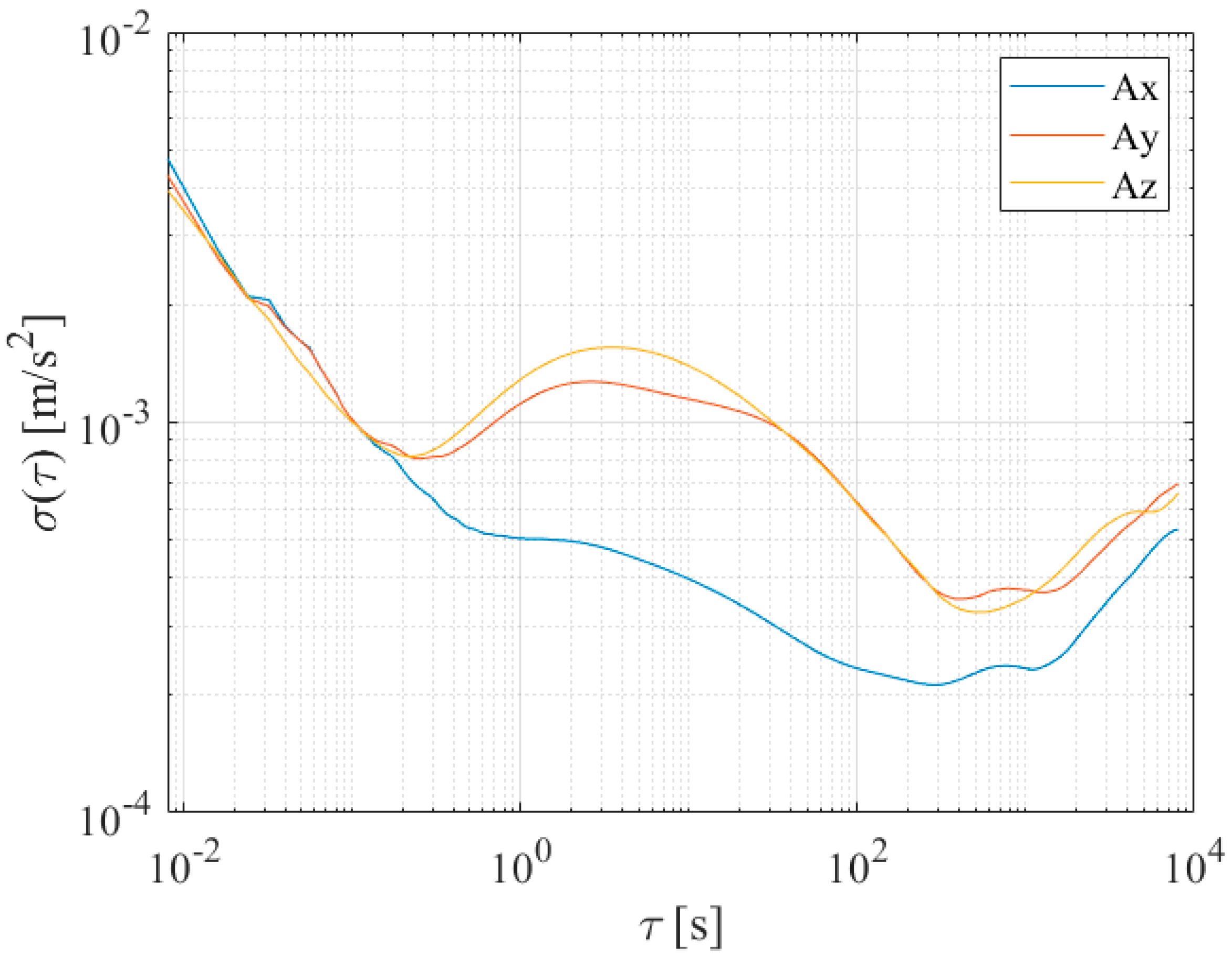
2.4. Allan Variance
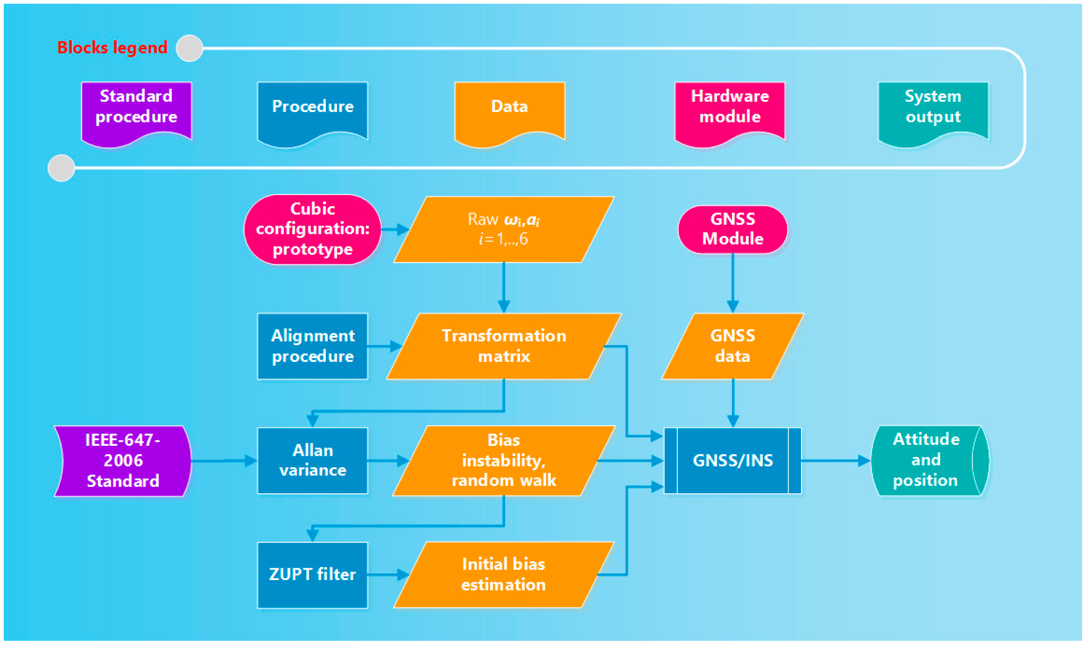
3. Proposed Method
3.1. Alignment Procedure
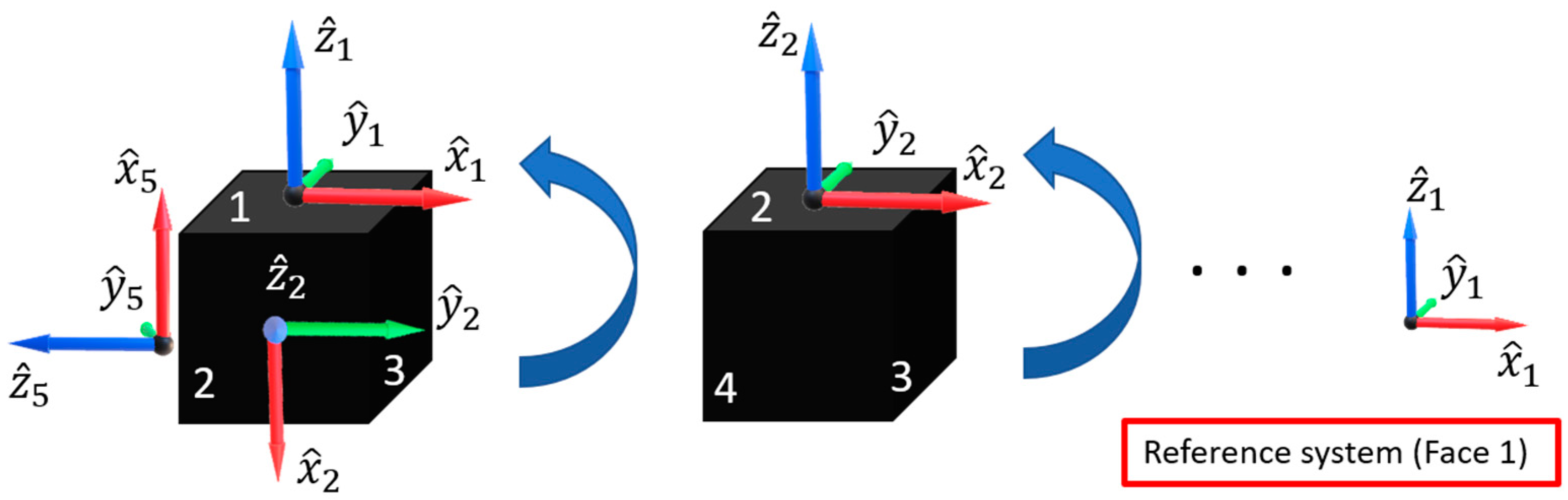
- The body frame of the inertial sensors installed on the face 1 of the cube is (arbitrarily) chosen as the reference frame the sensing axes of the other sensors are resolved to (Figure 3).
- Six rotations are applied to the cube in such a way as each face of the cube is positioned with an orientation coincident with that original of face 1. As an example, in the second step of Figure 3, the second rotation (associated with the face 2) is reported;
- For each rotation i (varying from 1 up to 6), raw data of acceleration are acquired from each sensor j (varying from 1 up to 6); the index k is associated with the acquired samples (varying from 1 up to N, N being the number of measurements carried out in each rotation);
- The average acceleration vector associated with the i-th rotation is calculated for each sensor and the results are normalized according towhere mean(·) stands for the average operating on each axis and norm(·) represents the traditional norm operator for vectors;
- The reference matrix V is arranged by means of acceleration components associated with face 1; in particular, the entries of the i-th row of the matrix V are equal to the components of the normalized acceleration of the rotation i
- As for the matrices Wj, their entries can be determined in a similar way
- According to the procedure presented in Section 2.2, a MATLAB® algorithm is performed to evaluate the alignment matrices. In particular, once the matrix is calculated according to Equation (8) for each face, the optimal rotation (i.e., that capable of making the j-th reference frame as close as possible to the first one) is determined as a quaternion (eigenvector) corresponding to the maximum eigenvalue of the Equation (7).
- Finally, the optimal quaternion is transformed in the related rotation matrix by means of straightforward calculation; obtained matrices are exploited to align all the measured inertial quantities to the reference frame of face 1.
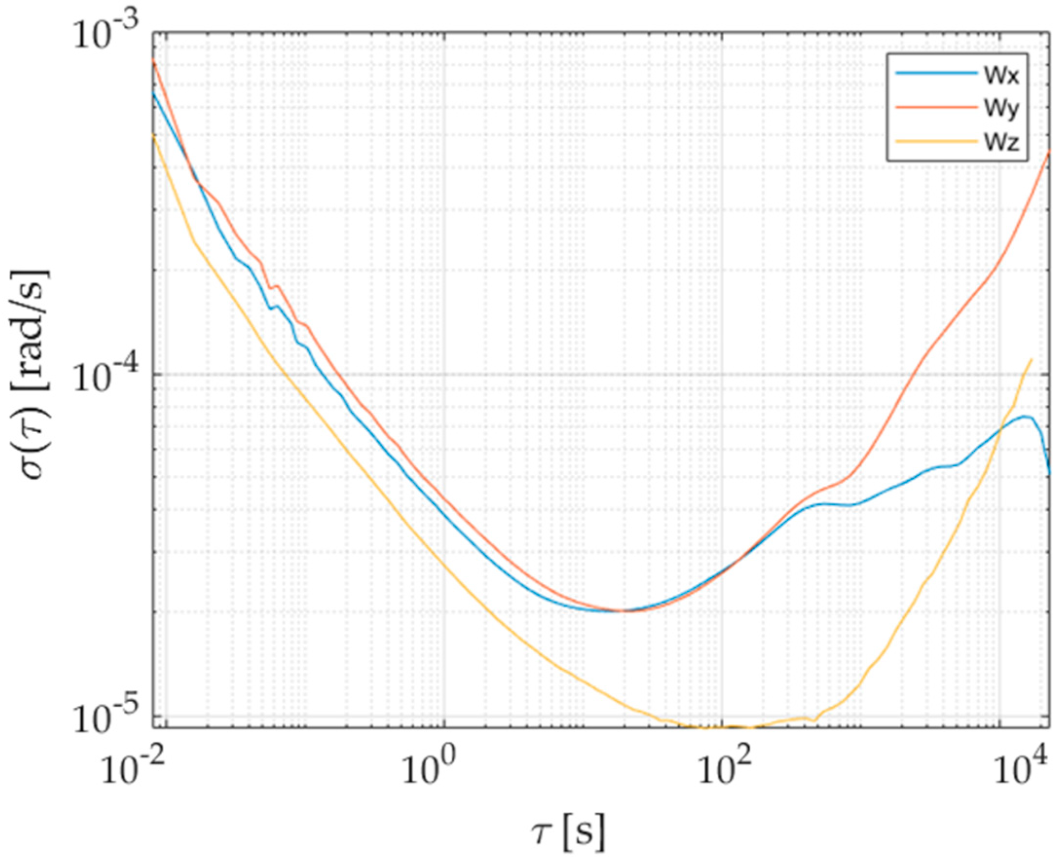
3.2. Noise Parameter Determination
3.3. Initial Biases Estimation
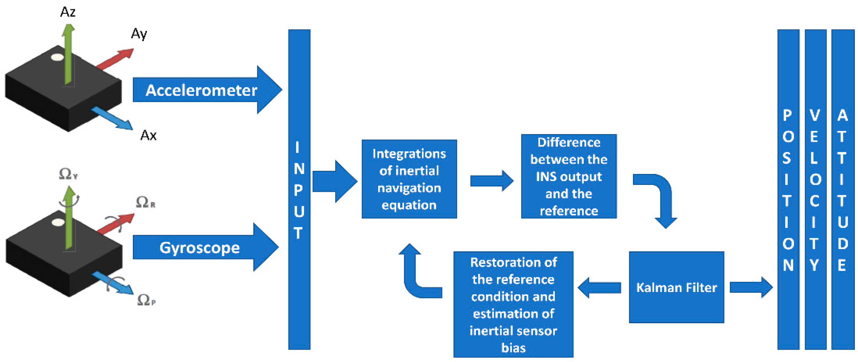
3.4. Kalman Filter-Based Navigation Algorithm
- Prediction/integration. At this step, the inertial navigation equations are integrated. To this aim, measures of accelerations and angular rates provided by the cube are first corrected from the last available values of bias. This stage provides the so-called a priori estimates of the state vector, i.e., a state vector updated by only integrating the corrected accelerations and angular rates; possible uncompensated biases effects make the estimated navigation parameters diverge from the actual values;
- Correction through GNSS data. When new measures of position and velocity are available from the GNSS, their values can be exploited to correct the a priori estimates of the state vector. In particular, a suitable matrix, Kalman gain, allows us to weight the confidence between integration and GNSS data and evaluate the so-called a posteriori estimate of the state vector. The higher the values of the Kalman gain, the greater the confidence and successive correction from GNSS measures with respect to the result of the integration stage. Moreover, in this step, the biases responsible for the difference between the integration and GNSS navigation parameters are estimated and given as input for the successive prediction/integration step.
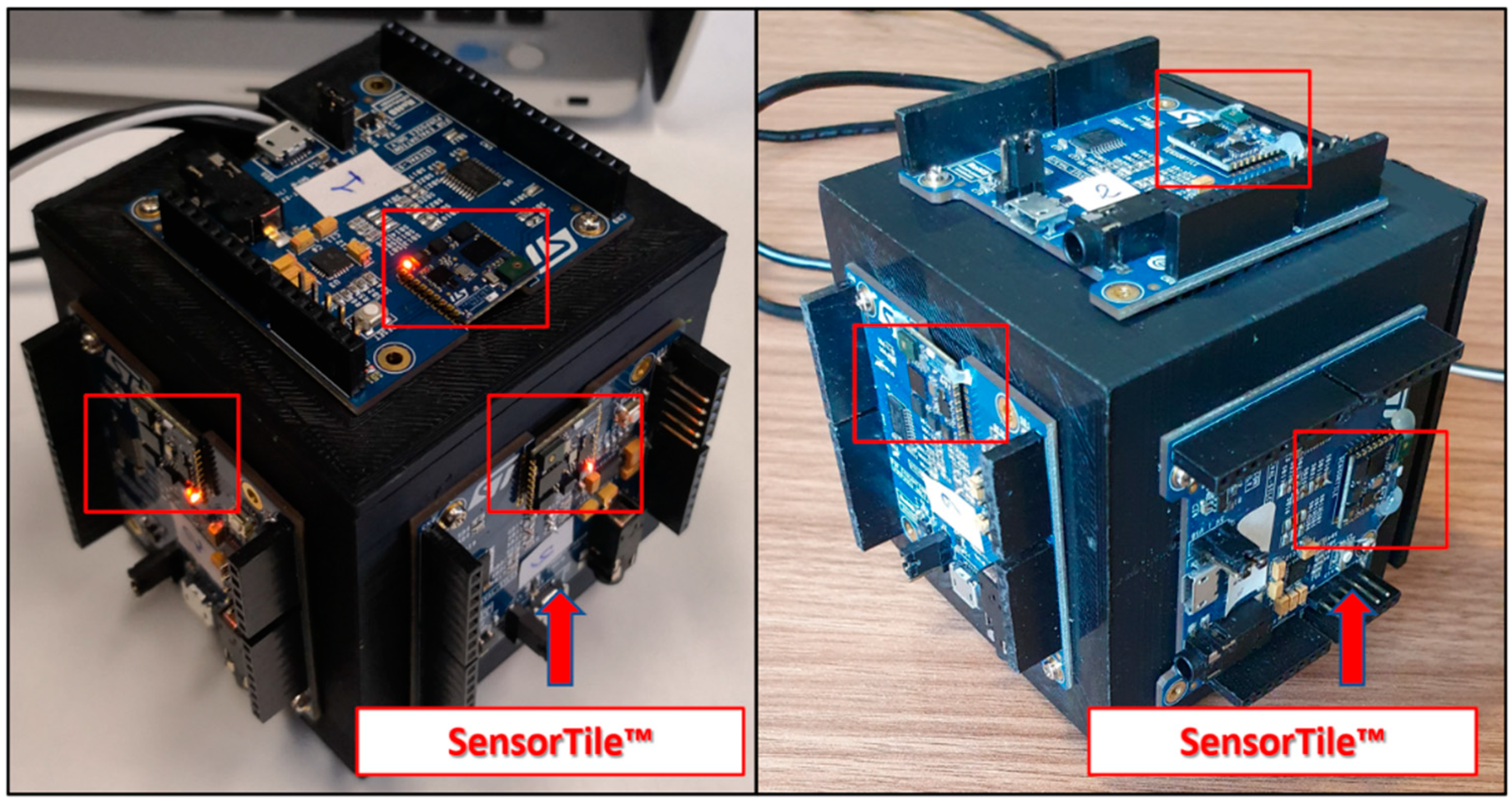
4. Realized Prototype of Redundant IMU
4.1. Hardware Architecture
4.2. Software Architecture
5. Experimental Results
5.1. Reference IMU
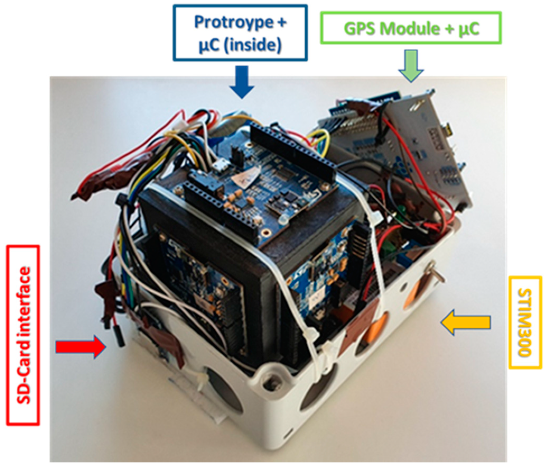
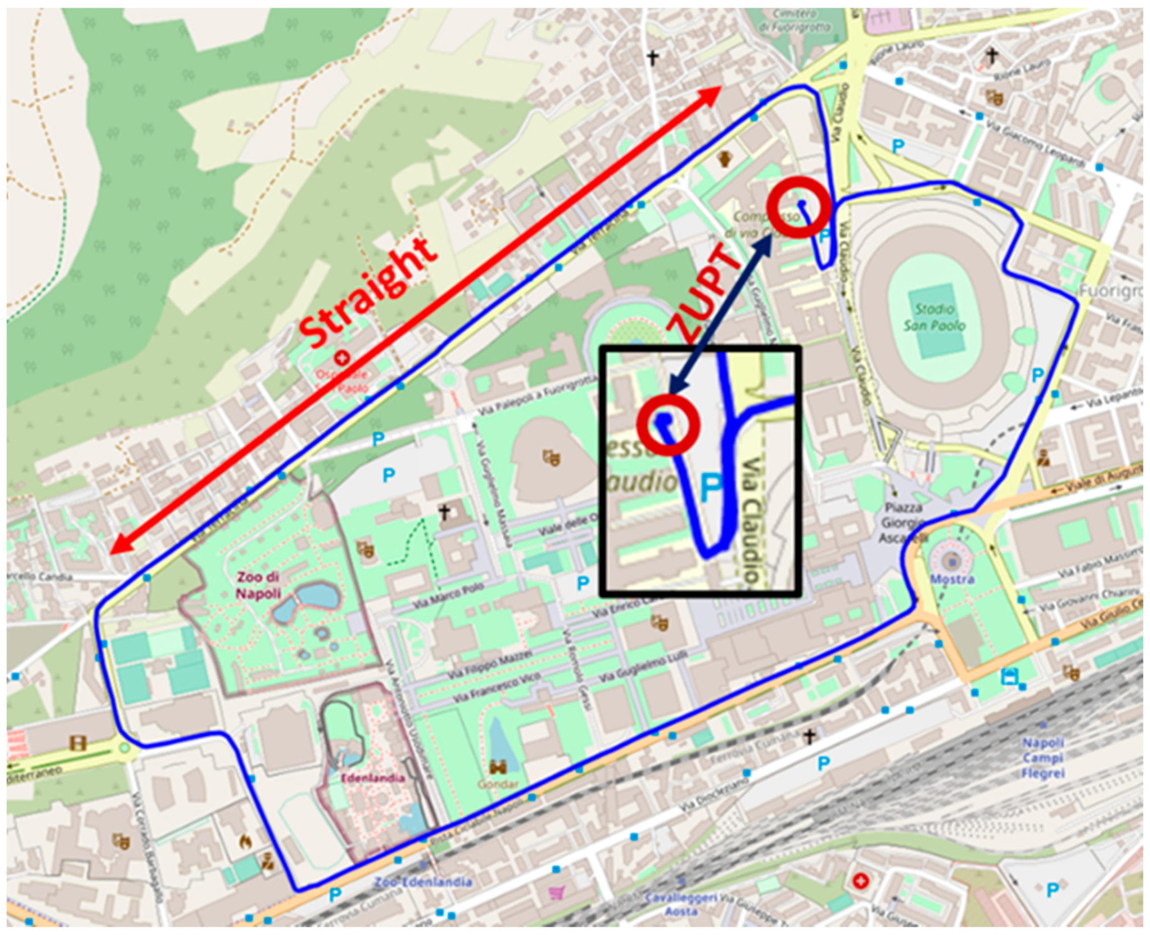
5.2. Measurements Setup for On-Field Tests
- 7.4 V and 2000 mAh battery for general power supply;
- DC-DC (Direct Current) step down converter circuit, to provide the adequate supply voltage for the exploited electronics;
- STIM300, used as reference IMU;
- Prototype of redundant IMU;
- GNSS module and its antenna;
- Status indicator LED;
- Two SDCard interfaces.
5.3. Preliminary Prototype Characterization
- stands for the gravity vector measured by the triaxial accelerometer mounted on the j-th face of the cube, aligned with face 1 after the i-th rotation;
- stands for the gravity vector measured by the triaxial accelerometer mounted on the 1st (reference) face of the cube after the i-th rotation;
- represents the traditional vector modulus operator.
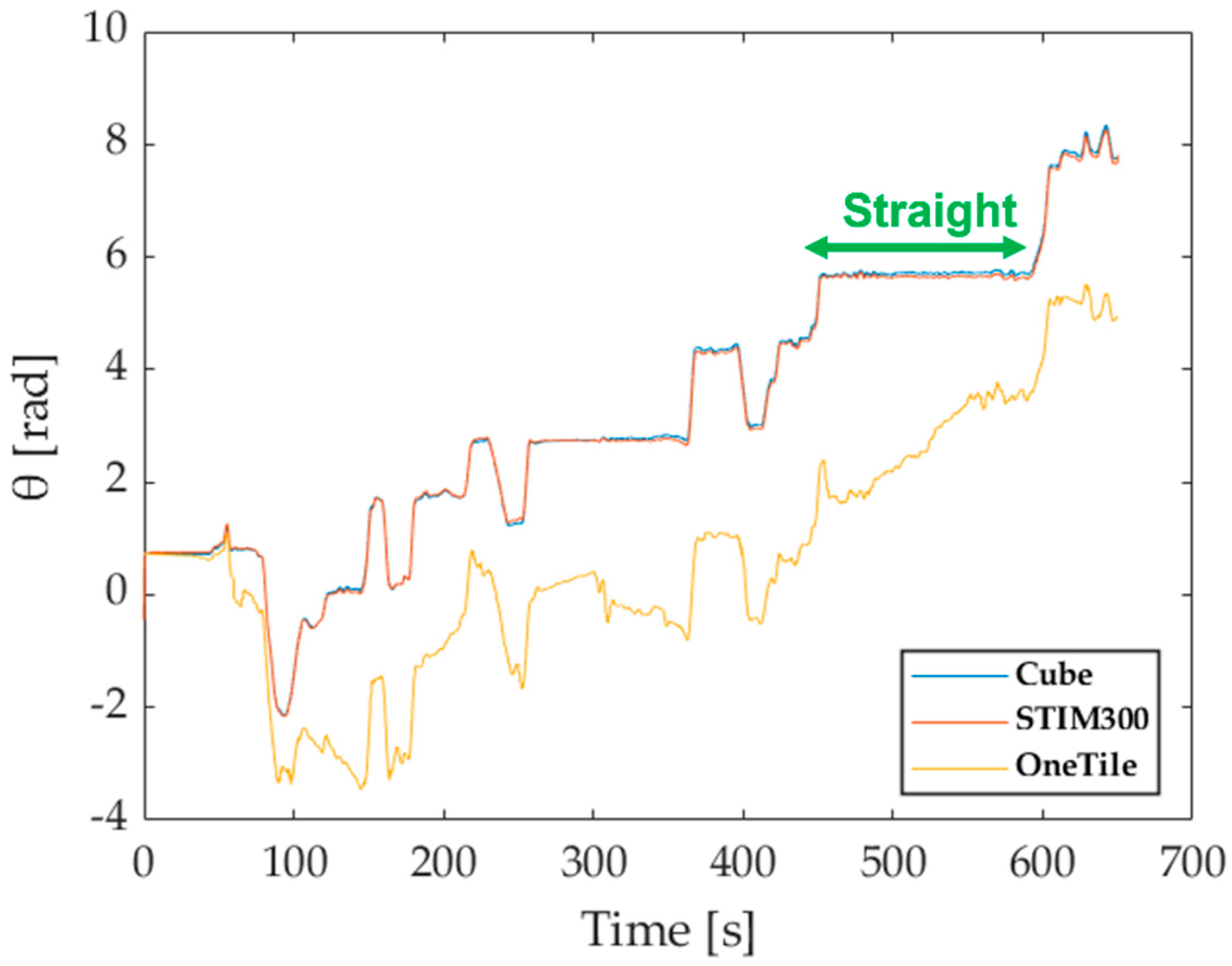
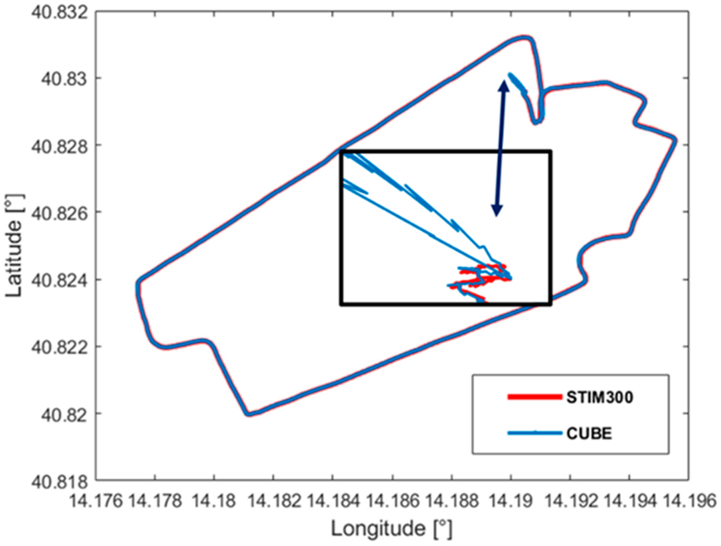
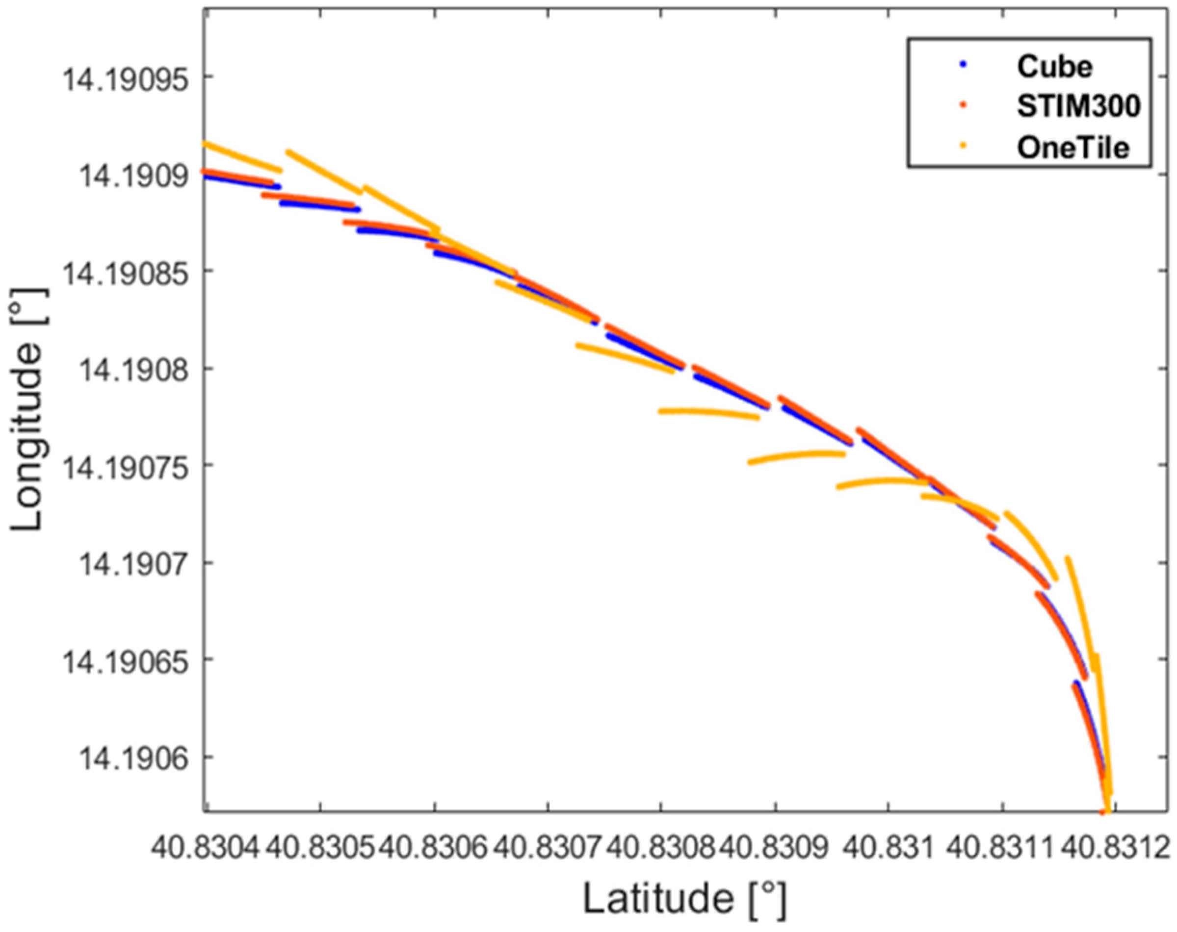
5.4. Attitude and Position
6. Conclusions
Author Contributions
Funding
Institutional Review Board Statement
Informed Consent Statement
Acknowledgments
Conflicts of Interest
References
- Lim, Y.; Gardi, A.; Sabatini, R.; Ramasamy, S.; Kistan, T.; Ezer, N.; Vince, J.; Bolia, R. Avionics Human-Machine Interfaces and Interactions for Manned and Unmanned Aircraft. Prog. Aerosp. Sci. 2018, 102, 1–46. [Google Scholar] [CrossRef]
- Carsten, O.; Martens, M.H. How can humans understand their automated cars? HMI principles, problems and solutions. Cogn. Technol. Work 2019, 21, 3–20. [Google Scholar] [CrossRef] [Green Version]
- Howard, D. Public Perceptions of Self-driving Cars: The Case of Berkeley, California. MS Transp. Eng. 2014, 14, 1–16. [Google Scholar]
- Ahvenjärvi, S. The Human Element and Autonomous Ships. TransNav Int. J. Mar. Navig. Saf. Sea Transp. 2017. [Google Scholar] [CrossRef] [Green Version]
- Groves, P.D. Principles of GNSS, inertial, and multisensor integrated navigation systems. IEEE Aerosp. Electron. Syst. Mag. 2015, 30, 26–27. [Google Scholar] [CrossRef]
- Savage, P.G. Strapdown Analytics; Strapdown Associates Inc.: Maple Plain, MN, USA, 2000. [Google Scholar]
- Wang, Z.; Cheng, X.; Du, J. Thermal Modeling and Calibration Method in Complex Temperature Field for Single-Axis Rotational Inertial Navigation System. Sensors 2020, 20, 384. [Google Scholar] [CrossRef] [PubMed] [Green Version]
- Ristic, B.; Arulampalam, S.; Gordon, N. Beyond the Kalman Filter: Particle Filters for Tracking Applications; Artech House: London, UK, 2004. [Google Scholar]
- Xu, H.; Yu, W.; Griffith, D.; Golmie, N. A Survey on Industrial Internet of Things: A Cyber-Physical Systems Perspective. IEEE Access 2018, 6, 78238–78259. [Google Scholar] [CrossRef]
- Marco, V.R.; Kalkkuhl, J.; Raisch, J.; Seel, T. A Novel IMU Extrinsic Calibration Method for Mass Production Land Vehicles. Sensors 2021, 21, 7. [Google Scholar] [CrossRef]
- Lee, J.S.; Jang, S.W.; Choi, J.G.; Lee, T.G. North-finding system using multi-position method with a two-axis rotary table for a mortar. IEEE Sens. J. 2016, 16, 1. [Google Scholar] [CrossRef]
- Niu, X.; Li, Y.; Zhang, H.; Wang, Q.; Ban, Y. Fast Thermal Calibration of Low-Grade Inertial Sensors and Inertial Measurement Units. Sensors 2013, 13, 12192–12217. [Google Scholar] [CrossRef]
- Passaro, V.M.N.; Cuccovillo, A.; Vaiani, L.; De Carlo, M.; Campanella, C.E. Gyroscope Technology and Applications: A Review in the Industrial Perspective. Sensors 2017, 17, 2284. [Google Scholar] [CrossRef] [PubMed] [Green Version]
- Microelectronics, S.T. User Manual-Getting Started with the STEVAL-STLKT01V1 SensorTile Integrated Development Platform. Available online: https://www.st.com/resource/en/user_manual/dm00320099-getting-started-with-the-stevalstlkt01v1-sensortile-integrated-development-platform-stmicroelectronics.pdf (accessed on 20 May 2021).
- Fontanella, R.; de Alteriis, G.; Accardo, D.; Moriello, R.S.L.; Angrisani, L. Advanced low-cost integrated inertial systems with multiple consumer grade sensors. In Proceedings of the AIAA/IEEE Digital Avionics Systems Conference, London, UK, 23–27 September 2018; Volume 2018. [Google Scholar] [CrossRef]
- IEEE. Aerospace and Electronic Systems Society (Institution). In Proceedings of the IEEE Standard Specification Format Guide and Test Procedure for Single-Axis Laser Gyros; IEEE Std 647-2006; IEEE Standard Association: Piscataway, NJ, USA, 2006. [Google Scholar]
- Titterton, D.; Weston, J.L.; Weston, J. Strapdown Inertial Navigation Technology; IET: London, UK, 2004; Volume 17. [Google Scholar]
- Waegli, A.; Guerrier, S.; Skaloud, J. Redundant MEMS-IMU integrated with GPS for performance assessment in sports. IEEE/ION Position Locat. Navig. Symp. 2008, 1260–1268. [Google Scholar] [CrossRef] [Green Version]
- Cai, G.; Chen, B.M.; Lee, T.H. Unmanned Rotorcraft Systems; Springer Science & Business Media: Berlin/Heidelberg, Germany, 2011. [Google Scholar]
- Wertz, J.R. Spacecraft Attitude Determination and Control; Astrophysics and Space Science Library; Springer: Berlin/Heidelberg, Germany, 2002. [Google Scholar]
- Jarrell, J.; Gu, Y.; Seanor, B.; Napolitano, M. Aircraft Attitude, Position, and Velocity Determination Using Sensor Fusion. In Proceedings of the AIAA Guidance, Navigation and Control Conference and Exhibit; American Institute of Aeronautics and Astronautics: Reston, VA, USA, 2008. [Google Scholar] [CrossRef]
- Chui, C.K.; Chen, G. Kalman Filtering with Real-Time Applications, 5th ed.; Springer: Berlin/Heidelberg, Germany, 2017. [Google Scholar]
- Gottschalg, G.; Leinen, S. Comparison and Evaluation of Integrity Algorithms for Vehicle Dynamic State Estimation in Different Scenarios for an Application in Automated Driving. Sensors 2021, 21, 1458. [Google Scholar] [CrossRef]
- Gonzalez, R.; Dabove, P. Performance Assessment of an Ultra Low-Cost Inertial Measurement Unit for Ground Vehicle Navigation. Sensors 2019, 19, 3865. [Google Scholar] [CrossRef] [PubMed] [Green Version]
- Liu, W.; Song, D.; Wang, Z.; Fang, K. Comparative Analysis between Error-State and Full-State Error Estimation for KF-Based IMU/GNSS Integration against IMU Faults. Sensors 2019, 19, 4912. [Google Scholar] [CrossRef] [PubMed] [Green Version]
- Gross, J.; Gu, Y.; Napolitano, M. A Systematic Approach for Extended Kalman Filter Tuning and Low-Cost Inertial Sensor Calibration within a GPS/INS Application. In Proceedings of the AIAA Guidance, Navigation, and Control Conference; American Institute of Aeronautics and Astronautics: Reston, VA, USA, 2010. [Google Scholar] [CrossRef]
- De Alteriis, G.; Conte, C.; Moriello, R.S.L.; Accardo, D. Use of consumer-grade MEMS inertial sensors for accurate attitude determination of drones. In Proceedings of the 2020 IEEE 7th International Workshop on Metrology for AeroSpace (MetroAeroSpace), Pisa, Italy, 22–24 June 2020. [Google Scholar] [CrossRef]
- Fontanella, R.; de Alteriis, G.; Moriello, R.S.L.; Accardo, D.; Angrisani, L. Results of field testing for an integrated gps/ins unit based on low-cost redundant mems sensors. In Proceedings of the AIAA Scitech 2019 Forum, San Diego, CA, USA, 7–11 January 2019. [Google Scholar] [CrossRef]
- Cheng, J.; Dong, J.; Landry, R.J.; Chen, D. A Novel Optimal Configuration form Redundant MEMS Inertial Sensors Based on the Orthogonal Rotation Method. Sensors 2014, 14, 13661–13678. [Google Scholar] [CrossRef] [PubMed] [Green Version]
- Wahba, G. A Least Squares Estimate of Satellite Attitude. SIAM Rev. 1965. [Google Scholar] [CrossRef]
- Hasan, A.M.; Samsudin, K.; Ramli, A.R.; Azmir, R.S.; Ismaeel, S.A. A Review of Navigation Systems (Integration and Algorithms). Aust. J. Basic Appl. Sci. 2009, 3, 943–959. [Google Scholar]
- Feng, X.; Zhang, T.; Lin, T.; Tang, H.; Niu, X. Implementation and Performance of a Deeply-Coupled GNSS Receiver with Low-Cost MEMS Inertial Sensors for Vehicle Urban Navigation. Sensors 2020, 20, 3397. [Google Scholar] [CrossRef] [PubMed]
- Xu, Q.; Li, X.; Chan, C. Enhancing Localization Accuracy of MEMS-INS/GPS/In-Vehicle Sensors Integration during GPS Outages. IEEE Trans. Instrum. Meas. 2018, 67, 1966–1978. [Google Scholar] [CrossRef]
- STMicroelectronics. iNemo–Inertial Module Datasheet. March 2015. Available online: https://www.st.com/resource/en/datasheet/lsm6dsl.pdf (accessed on 20 May 2021).
- STMicroelectronics. Teseo-LIV3F Datasheet. April 2019. Available online: https://www.st.com/resource/en/datasheet/teseo-liv3f.pdf (accessed on 20 May 2021).
- Mbed-Rapid IoT Device Development. Available online: https://www.os.mbed.com (accessed on 20 May 2021).
- SensoNor, STIM300 Datasheet, Rev. 9 TS1524. May 2013. Available online: https://www.sensonor.com/products/inertial-measurement-units/stim300/ (accessed on 20 May 2021).
- De Alteriis, G.; Accardo, D.; Moriello, R.S.L.; Ruggiero, R.; Angrisani, L. Redundant configuration of low-cost inertial sensors for advanced navigation of small unmanned aerial systems. In Proceedings of the 2019 IEEE 5th International Workshop on Metrology for AeroSpace (MetroAeroSpace), Torino, Italy, 19–21 June 2019. [Google Scholar] [CrossRef]
- Choi, M.J.; Kim, Y.H.; Kim, E.J.; Song, J.W. Enhancement of Heading Accuracy for GPS/INS by Employing Average Velocity in Low Dynamic Situations. IEEE Access 2020, 8, 43826–43837. [Google Scholar] [CrossRef]
- Parsa, K.; Lasky, T.A.; Ravani, B. Design and Implementation of a Mechatronic, All-Accelerometer Inertial Measurement Unit. IEEE/ASME Trans. Mechatron. 2007, 12, 640–650. [Google Scholar] [CrossRef]
- Zhao, W.; Cheng, Y.; Zhao, S.; Hu, X.; Rong, Y.; Duan, J.; Chen, J. Navigation Grade MEMS IMU for A Satellite. Micromachines 2021, 12, 151. [Google Scholar] [CrossRef] [PubMed]


| [°] | Face 2 | Face 3 | Face 4 | Face 5 | Face 6 |
|---|---|---|---|---|---|
| Mean Value | 0.68 | 0.84 | 0.72 | 0.69 | 0.32 |
| STD | 0.18 | 0.16 | 0.31 | 0.28 | 0.13 |
| Gyroscope Allan Parameter | Prototype | Single Sensor (Best) | ||
|---|---|---|---|---|
| BI [°/h] | ARW [°/] | BI [°/h] | ARW [°/] | |
| X-Axis | 3.1 | 0.11 | 5.7 | 0.24 |
| Y-Axis | 3.1 | 0.11 | 15.7 | 0.36 |
| Z-Axis | 1.8 | 0.12 | 3 | 0.24 |
| Accelerometer Allan Parameter | Prototype | Single Sensor (Best) | ||
|---|---|---|---|---|
| BI [mg] | VRW | BI [mg] | VRW | |
| X-Axis | 0.02 | 0.01 | 0.05 | 0.04 |
| Y-Axis | 0.02 | 0.02 | 0.09 | 0.05 |
| Z-Axis | 0.03 | 0.01 | 0.04 | 0.05 |
| Range Values [min-max] | Gyroscopes | Accelerometers | ||
|---|---|---|---|---|
| BI [°/h] | ARW [°/] | BI [mg] | VRW | |
| X-Axis | 5.7–73 | 0.21–0.25 | 0.05–0.08 | 0.04–0.07 |
| Y-Axis | 5.1–25 | 0.21–0.37 | 0.05–0.09 | 0.05–0.07 |
| Z-Axis | 3–15 | 0.24–0.36 | 0.05–0.1 | 0.04–0.08 |
| IMU | Prototype | Single Face (Range) | ||
|---|---|---|---|---|
| Angle [°] | Pitch | Roll | Pitch | Roll |
| Mean Value | 0.21 | 1.07 | −1.01 to 1.45 | 1.24 to 14.71 |
| STD | 0.09 | 0.31 | 0.11 to 0.45 | 0.2 to 0.61 |
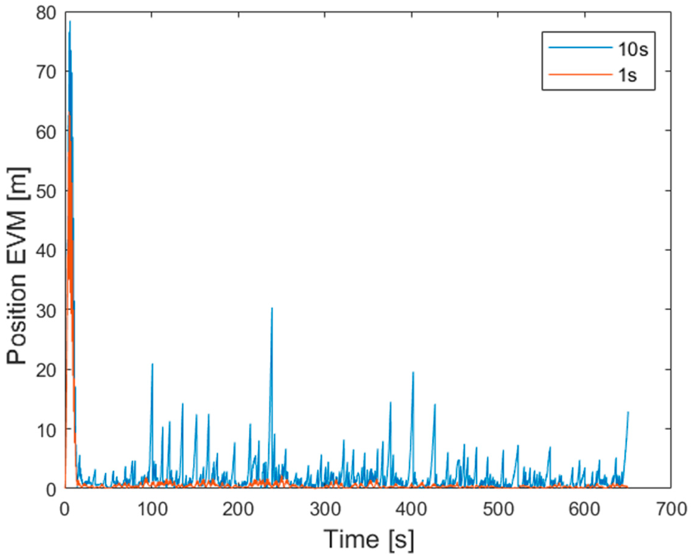
| GPS Outages | 1 s | 2 s | 5 s | 10 s | Random |
|---|---|---|---|---|---|
| Position RMSE [m] | 0.89 | 1.12 | 1.31 | 5.25 | 2.38 |
| Position RMSE Straight [m] | 0.63 | 0.84 | 1.03 | 3.12 | 1.72 |
| GPS Outages | 1 s | 2 s | 5 s | 10 s | Random |
|---|---|---|---|---|---|
| θ RMSE [rad] | 0.035 | 0.033 | 0.056 | 0.111 | 0.035 |
| θ RMSE Straight [rad] | 0.037 | 0.034 | 0.023 | 0.051 | 0.025 |
Publisher’s Note: MDPI stays neutral with regard to jurisdictional claims in published maps and institutional affiliations. |
© 2021 by the authors. Licensee MDPI, Basel, Switzerland. This article is an open access article distributed under the terms and conditions of the Creative Commons Attribution (CC BY) license (https://creativecommons.org/licenses/by/4.0/).
Share and Cite
de Alteriis, G.; Accardo, D.; Conte, C.; Schiano Lo Moriello, R. Performance Enhancement of Consumer-Grade MEMS Sensors through Geometrical Redundancy. Sensors 2021, 21, 4851. https://doi.org/10.3390/s21144851
de Alteriis G, Accardo D, Conte C, Schiano Lo Moriello R. Performance Enhancement of Consumer-Grade MEMS Sensors through Geometrical Redundancy. Sensors. 2021; 21(14):4851. https://doi.org/10.3390/s21144851
Chicago/Turabian Stylede Alteriis, Giorgio, Domenico Accardo, Claudia Conte, and Rosario Schiano Lo Moriello. 2021. "Performance Enhancement of Consumer-Grade MEMS Sensors through Geometrical Redundancy" Sensors 21, no. 14: 4851. https://doi.org/10.3390/s21144851
APA Stylede Alteriis, G., Accardo, D., Conte, C., & Schiano Lo Moriello, R. (2021). Performance Enhancement of Consumer-Grade MEMS Sensors through Geometrical Redundancy. Sensors, 21(14), 4851. https://doi.org/10.3390/s21144851